Software stability assessment using multiple prediction models

Université de Montréal

Software Stability Assessment Using Multiple

Prediction Models

Par

Hong Zhang

Le Département d’informatique et de recherche opérationnelle

Faculté des arts et des sciences

Mémorire présenté à la Faculté des études supérieures

En vue de l’obtention du grade de

Maîtrise ès sciences (M.Sc.)

En informatique

de Montréal

Direction des bibliothèques

AVIS

L’auteur a autorisé l’Université de Montréal à reproduire et diffuser, en totalité ou en partie, par quelque moyen que ce soit et sur quelque support que ce soit, et exclusivement à des fins non lucratives d’enseignement et de recherche, des copies de ce mémoire ou de cette thèse.

L’auteur et les coauteurs le cas échéant conservent la propriété du droit d’auteur et des droits moraux qui protègent ce document. Ni la thèse ou le mémoire, ni des extraits substantiels de ce document, ne doivent être imprimés ou autrement reproduits sans l’autorisation de l’auteur.

Afin de se conformer à la Loi canadienne sur la protection des

renseignements personnels, quelques formulaires secondaires, coordonnées ou signatures intégrées au texte ont pu être enlevés de ce document. Bien que cela ait pu affecter la pagination, il n’y a aucun contenu manquant.

NOTICE

The author of this thesis or dissertation has granted a nonexclusive license allowing Université de Montréal to reproduce and publish the document, in part or in whole, and in any format, solely for noncommercial educational and research purposes.

Ihe author and co-authors if applicable retain copyright ownership and moral

rights in this document. Neither the whole thesis or dissertation, nor

substantial extracts from it, may be printed or otherwise reproduced without the author’s permission.

In compliance with the Canadian Privacy Act some supporting forms, contact information or signatures may have been removed from the document. While this may affect the document page count, it does not represent any loss of content from the document.

Université de Montréal

Faculté des études supérieures

Ce mémoire de maîtrise intitulé

Software Stability Assessment Using Multiple

Prediction Models

Présenté par

Hong Zhang

A été évalué par un jury composé des personnes suivantes

Présidente rapporteur:

EL MABROUK, Nadia

Directeur de recherche :

SAHRAOUI, Houari

Membre

du

jury:

ABOULHAMID, El Mostapha

La qualité de logiciel est actuellement de plus en plus un souci des organizations. La manière la plus populaire d’assurer la qualité de logiciel est d’appliquer des modèles de prévision de qualité de logiciel. Les modèles de prévision peuvent aider dans l’évaluation de beaucoup d’aspects de qualité de logiciel pendant l’étape de développement de logiciel; par exemple, entretien, réutilisabilité, fiabilité et stabilité. En effet, les modèles de prévision deviennent une méthode efficace pour contrôler la qualité de logiciel avant que l’ensemble des progiciels soit déployé, ou pour prévoir la qualité du logiciel avant qu’il soit utilisé. Pendant les dix dernières années, beaucoup d’études liées à ce sujet ont été publiées et un grand nombre de modèles de prévision de qualité ont été proposés dans la littérature. Cependant, établir les modèles de prévision de qualité de logiciel est une tâche complexe et à ressources consumantes.

En général, il y a deux approches de base pour construire les modèles de prévision de qualité de logiciel. La première établit automatiquement le modèle avec des données historiques. La seconde fait participer des experts établissant le modèle manuellement.

La première approche se fonde sur des données de mesure historiques pour accomplir son but. La qualité de ces modèles dépend fortement de la qualité des échantillons utilisés. Malheureusement, la qualité des échantillons disponibles est habituellement pauvre en programmation. La quantité limitée de données disponibles pour ces modèles le rend difficile à généraliser, valider, et de réutiliser les modèles existants. En effet, contrairement à d’autres domaines, les petites tailles et l’hétérogénéité des échantillons de rendent très difficile de dériver des modèles largement applicables.

La connaissance extraite de l’heuristique domaine-spécifique est employée par la deuxième approche pour établir les modèles de prévision de qualité de logiciel. Les modèles obtenus emploient des jugements des experts, et vise à établir un rapport

intuitivement acceptable entre les attributs internes de logiciel et une caractéristique de qualité. Bien que ces modèles soient adaptés au processus décisionnaire, il est difficile de les généraliser faute de connaissance conrnrnne et largement admise dans le domaine de qualité de logiciel.

A cause du manque de données historiques ou de connaissance experte dans un domaine spécifique, il est difficile d’établir systématiquement les modèles de prévision spécifiques. Une alternative est de choisir un modèle de prévision existant. Mais les modèles spécifiques obtenus à partir d’une situation particulière ne sont pas assez généraux pour être efficacement applicables. Par conséquent, le choix d’un modèle approprié est une décision difficile et non triviale pour une compagnie.

Dans notre thèse, nous proposons une approche de combinaison pour résoudre ce problème. L’idée principale est de combiner et adapter les modèles existants de telle manière que le modèle combiné fonctionne bien sur un système particulier ou dans un type d’organisation particulier. En outre, nous visons également à améliorer les capacités de prévision des modèles existants.

L’approche de combinaison est recommandée comme une manière efficace pour améliorer les modèles de simple-issue utilisés actuellement. Nous employons un algorithme génétique pour mettre en application notre approche de combinaison. Dans notre solution proposée, nous supposons que les modèles de prévision existants sont l’arbre de décision ou les classificateurs basés sur les règles. Les résultats d’essai indiquent que l’approche de combinaison proposée avec un algorithme génétique peut améliorer les capacités de prévision des modèles existants de manière significative dans un contexte de systèmes multiple.

Mote clés Modèle de Prévision de Qualité de Logiciel, Métrique Logiciel, Algorithme Génétique

Software quality is a concem of more ami more organizationsnow. The most popular way to assure software quality at present is to appty software quality prediction models. Prediction models can help in the evaluation of many aspects of software quality during the software development stage; such as, maintainability, reusability, reliability and stability. In fact, prediction models are becoming an efficient way to control software quality before software packages are deployed, or to predict the quality of the software before they are used. During the past tel years, a lot of studies related to this subject have been published and a large number of quality prediction models have been proposed in the literature. However, building software quality prediction models is a complex and resource-consurning task.

In general, there are two basic approaches to building software quahty prediction models. The first one uses historical data to build the model autornatically. The second one involves experts building the model manually.

The first approach relies on historical measurement data to accomplish its goal. The quality of these models depends heavily on the quality of the samples used. Unfortunately, the quality of samples available is usually poor in software engineering. The lirnited amount of data available for these models makes it difficuit to generalize, to cross-validate, and to reuse existing models. lndeed, contrary to other domains, the small sizes and the heterogeneity ofthe samples makes it very difficuit to derive widely applicable models.

Knowledge extracted from domain-specific heuristics is used by the second approach to build software quality prediction models. The obtained prediction models use judgments from experts, and aim to establish an intuitively acceptable causal relationship between internaI software attributes and a quality characteristic. Although

these models are adapted to the thought decision-making process, they are also hard to generalize because of a lack of widely accepted common knowledge in the ficld of software quality.

Due to the Ïack of historical data or the lack of expert lmowledge in a specific domain, it is hard to build organizationally specific prediction models. An alternative can be to choose an existing prediction mode!. But the specific models obtained from a particular situation are flot general enough to be efficicntly applicable. As a consequence, selecting an appropriate quality mode! is a difficuit and non-trivial decision for a company.

In our thesis, we propose a combination approach to solve this problem. The main idea is to combine and adapt existing models in such a way that the combined model works well on a particular system or in a particular type of organization. In addition we also aim at improving the prediction ability of existing models.

The combination approach is recommended as an efficient way to improve on the single-issue models used at present. We use a genetic algorithm to implement our combination approach. For our proposed solution, we assume that the existing prediction models are the decision tree or rnle-based classifiers. The test results indicate that the proposed combination approach with a genetic algorithm can significantly improve the prediction ability of existing models within a multiple systems context.

Abstract

Résumé

Contents

V

List of Figures

List of Tables

Acknowledgements

Chapter 1

Introduction

Chapter

2 Software Quality Prediction Models

2.1 Terminology of Software Quality 7

2.2 Software Quality Assurance 9

2.3 Software Measurement and Metrics 11

2.4 Software Quality Prediction Models and Building Approach 1$

2.5 Existing Software Quality Prediction Models 20

2.5.1 Statistical/Regrcssion Modes 21

2.5.2 BBN Models 23

2.5.3 Neural Network Models 26

2.5.4 Decision Tree Models 28

2.6 Summary ofthis Chapter 32

Chapter 3 Genetic Algorithm Principles

3.1 Introduction ofGenetic Algorithm Principles 33

3.2 Terms of Genetic Algorithm 35

3.2.2 Genotype and Phenotype .37

3.2.3 Generation and Population 3$

3.2.4 Fitness _3$

3.2.5 Search Space 39

3.3 The Genetic Algonthm Operators 39

3.3.1 Selection ₃₉ 3.3.2 Crossover 42 3.3.3 Mutate ₄₄ 3.3.4 Elitism ₄₅ 3.4 Parameters ₄₅ 3.4.1 Population Size 45 3.4.2 Crossover Probability 45 3.4.3 Mutation Probability 46

3.5 Three Stages ofa Genetic Algonthm Application 46

3.6 Summary ofthis Chapter 47

Chapter 4 Combination Algorithm

4.1 Research Methodology 4$

4.2 Data Environment 49

4.3 Model Coding ₅₃

4.3.1 Representation ofModels 53

4.3.2 Representation of Basic Rule and Default Rule 54

4.4 Initial Generation ₅₆

4.5 Combination Algorithm Operators 57

4.5.1 Selection 57

4.5.2 Crossover 59

4.5.3 Mutation 65

4.6 Fitness Function ₆₉

4.7 Elitism ₇₂

4.8 Control of Population Size 72

4.9 Ending Condition 73

4.10 The Main Generational Loop in Our Algorithm 74

5.1 Experimental bol: GA-CAMP 77

5.2 Stability 82

5.3 Source Data Sets and Models Extract 84

5.4 Experiment Settings 89

5.5 Case Study 91

5.5.1 Case Study 1 92

5.5.2 Case Study 2 93

5.5.3 Case Study Summary 94

5.6 Resuits ₉₄

5.7 Sumrnary ofthis Chapter 98

Chapter 6 Conclusion

6.1 Sumrnary ₉₉

6.2 Future work 101

Bibliography

Appcndix A

LIST 0F FIGURES

Figure 1.1 The Approach and Concept of Our Research 4

figure 2.1 The V Model for Quality 10

figure 2.2 Predictor and Control Metrics 12

Figure 2.3 Relationships Between Internai and External Software Attributes 16

figure 2.4 “Reliability Prediction” BNN Example 25

Figure 2.5 A Neural Network Estimation Model 2$

figure 2.6 A Decision Tree Diagram 29

Figure 2.7 A Decision Tree for Stability Prediction 31

Figure 2.8 A Rule Set Translated from Figure 2.7 32

Figure 3.1 Chromosome Pair Nature Shape and Representation in Our Study 36

Figure 3.2 The Binary Representation ofa Chromosome 37

Figure 3.3 Genotype and Phenotype in Nature 38

Figure 3.4 Roulette Wheel 40

Figure 3.5 Rank Selection 41

Figure 3.6 Crossover (cutting point 5, fixed length) 43

figure 3.7 Mutation 44

figure 4.1 A Classic Rule-Based Prediction Model for Stability 50 Figure 4.2 The Example ofa Basic Rule (Gene) in Model 1 51

Figure 4.3 The Rule-Based Prediction Model Structure 52

figure 4.4 A Chromosome Internai Structure in Biology 53 figure 4.5 The Representation ofModel 1 as a Chromosome 54 figure 4.6 Representations of a Chromosome and its Genes by a Model 54 figure 4.7 Exampie ofthe Internai Structure ofa Gene (for Basic Rule) 55

figure 4.8 A Basic Rule Structure 55

f igure 4.9 Structure ofa Condition 55

figure 4.10 Roulette Wheel for Selection 5$

Figure 4.11 Crossover of Model 4 and Model 13 with One Cutting Point 61 f igure 4.12 Two Original Models (Model 4 and Model 13) 62

Figure 4.13 Two New Models afier Crossover 63

figure 4.14 Two Cutting Points Crossover 64

Figure 4.17 A Condition Mutated in Figure 4.16 67 Figure 5.1 The Combination Algorithm Interface of GA-CAMP 78 Figure 5.2 An Example of Decision Tree Classifier File Produced by C4.5 79 Figure 5.3 A Rule Set ofa Decision Tree Crcated by C4.5 88 Figure 5.4 The Original and Combination Models’ fitness on Training Data 96 Figure 5.5 The Original and Combination Models’ Fitness onTesting Data 96

LIST 0F TABLES

Table 2.1 Software Characteristics from ISO/IEC 9216 11

Table 2.2 Function-Onented Software Product Metrics 14

Table 2.3 Object-oriented Metries 15

Table 2.4 The 22 Software Metrics Used as Attributes in Our Expenments 18

Table 4.1 The Metrics Database and Values 68

Table 4.2 The Confusion Matrix of a Decision function 69 Table 4.3 Confusion Matrix and Fitness Function for this Study 70

Table 4.4 Data Environment 71

Table 5.1 The Software Systems Used to Train and to Combine the Models 84 Table 5.2 The 22 Software Metrics Used as Attributes in Our Experiment 85 Table 5.3 The 10 Repetitions 0fExperiment Data Environments 90

Table 5.4 GA-CAMP Parameters 91

Table 5.5 The Results ofthe first Experiment 92

Table 5.6 The Resuits ofthe Second Experiment 93

Table 5.7 Fitness Values from Training and Testing Data 94

I would like to express my sincere appreciation to my director, Dr. Houari Sahraoui for

his invaluable guidance, his encouragement, his care and support throughout the course

of this thesis work. I really appreciate the opportunity to work on such an interesting

project with his guidance and advice. He has constantly supported me in a very kind and

encouraging way by pointing out relevant research and generating interesting ideas.

I also would like to make a special acknowledgernent to Mr. Salah Bouktif for his

collaboration in the development and implementation of the Algorithms. I benefited

greatly

_{fonnal and informai discussions with him. I am also thankful to Mr.}

Moharnmed Rouatbi, who offered me his efficient fitness function used by the genetic

algorithm.

I also truly thank my brother Zhang Yi Wei. This thesis has benefited from his careful

reading and constructive criticisrn.

I also express my thanks to my friends Chen Ji Ling, Qin Li Sheng, Shen Shi Qiang, Mai

Gang, Zheng Suo Shi and Wu Lei for their help, friendship and encouragement.

Finally, I wish to express a speciai acknowledgement to my wife Jia Dong Mei, my

daughter Yue Ran Zhang and my son Gary Zhang for their support, understanding, and

for making alt of this possible.

Chapter 1

Introduction

1.1 Motivation

Comptiter use is now prevalent in almost ail aspects of our everyday life; consequently, software has become criticai to the deveiopment and maintenance of consumer products. Now, more than ever, software developers are concemed with software quality when developing new products. The reason for this stems from the immense demands on peopie, money and time when developing software products because software is becoming iarger and more complex [35]. The question of how to develop high-quaiity software is critical. One of the best ways to assure software quality is to address this issue and make accurate predictions before the software is developed.

Predicting software quality is a compiex and resource-consuming task. The process of predicting defects in the eariy stage of the software iifecycle has become a major undertaldng for software engineers. Over the iast 30 years a great deal ofresearch has been undertaken in an attempt to predict software quality [24]. There are many papers advocating statistical models and metrics which purport to answer the quaiity question. Many of the studies related to this issue have added to our knowiedge base. For example, numerous software metrics have been developed and some of the prediction modeis buiit from these metrics have been found to be effective toois in controiling the software quaiity. In fact, prediction modeis are becoming an efficient way to controi

Recently, many prediction models have been proposed to predict certain aspects of software quaiity: such as, maintainability, reusability, reliability, and stability to name a few [24]. Most of these prediction models have been buiit using statistical methods, which require historical data. Unfortunateiy, many software developers lack historical data. Therefore, it is hard to build organizationally specific prediction models because of this lack of information. Consequently, the alternative has been to choose existing prediction models. However existing models are specific to a particular situation and consequentiy are flot general enough to be efficiently applied to other contexts. More significantly, many prediction modeis tend to model only part of the underlying problem within a context: therefore, they are not universai. Intuitivety, a way to solve this problem might be by coliecting data from different kinds of application contexts to build universal software quality prediction moUds. Unfortunateiy, this wouid be too complex and too time consuming to achieve. furthermore, in practice, it’s aimost impossible to obtain ail the data necessary for prediction models to be built. Therefore, in our research, we hope to address these problems by proposing a combination algorithm to obtain a cross-valid software quaiity prediction model.

1.2 Goals

In generai, software quaiity prediction models are obtained from historical measurement data or the domain specific heuristics of experts. The main purpose ofthis research is to find another approach to establishing quality prediction models through the combination of existing models in order to obtain new modes. This new prediction model is neither from the historical measurement data nor from experts’ knowledge.

The combined models obtained from existing prediction models can be an alternative for software organizations that lack historical data. This approach is achievable because many prediction modeis, which can oniy satisfactorily work for the specific circumstances from which they were built, have been proposed inthe last few decades.

Chaptet 1 3

We propose an approach that combines these existing prediction models from various contexts, using a genetic algorithm, with the goal being to produce a more universally applicable “combining model” for software stability prediction. The results obtained from this study show that this approach is more efficient and the prediction accuracy is higher in the testing data sets.

Therefore, flot only has it become effective and efficient to produce a predictive model from the existing predictive models of these organizations. Their results can lead to higher prediction accuracy rate that requires less effort during the implementation phase and makes the design phase more efficient.

The “combining model” approach is illustrated in figure 1.1. Each cylinder indicates the source data set from which the prediction models are built. Each rectangle indicates the approach to building the prediction models. Each ellipse indicates the prediction model. In the literature, only the prediction models and some of the approaches are presented. That is, the sotirce data sets are unknown. This research focuses on the stability rnle-based prediction models. Our aim is to find an approach to build a new model from the posted models using a genetic algorithm. It is hoped that both this approach and this new model can be applied widely. Using this new approach, it is not necessary to have the original source data sets because our input data actually is a set of existing prediction models. Our outputs arc some ncw prediction models that are more general and more accurate in estimating software quality. Moreover, this study is also an exploratory phase that offers proofto the concept of combining existing models with the genetic algorithm. Somc techniques and results of this study have been improvcd by the students that continue the research [55].

Therefore, the goal ofthis study is to propose and verify the ‘combining’ approach, by using a genetic algorithm, as an efficient method to develop cross-valid software

unknown

known

Combination Algorithrn

New Prediction Model

Figure 1.1 The Approach and Concept of Our Research

1.3 Contributions

Our combination algorithm was validated in a “semi-reaF’ environment. In this evaluation environment, ail data collected was from some reai software systems and the models were extracted from part of this data set through the C4.5 aigorithm [51]. We trained the original models and tested the combination models with alO-fold cross validation technique in this real data environment also. The resuits coming from our experiment are: that a certain ldnd of local search method, such as a genetic algorithm, can be used as an evolutionaiy approach for combining and improving software quaiity prediction models in a particular context.

Our researcli contribution focuses on the foliowing two aspects:

first, we propose an approach to using a genetic algorithm for the improvement of prediction models through their combination.

Chapter 1

Second, we show that this approach can work well for the classes interface stability prediction in real software systems.

1.4 Outline

In this study, we apply a genetic algorithm (GA) as a combination approach to build more satisfactory software quality prediction models and optimize the prediction accuracy ofthe new models.

In Chapter 2, we present a review of the concepts of software quality and its prediction models, as well as a description of some software quality prediction models that have been posted in the literature in order to provide an example of other prediction models. In Chapter 3, we describe the GA principles in general, such as GA operators and parameters. The research methodology of our combination algorithm is presented in Chapter 4, while Chapter 5, describes the implementation of our experiment using the algorithm on the stability prediction models.

finally, in Chapter 6, conclusions are made and a brief summary is presented. Furthermore, problems conceming optimizing quality estimation models with this specific technique and future work are presented.

Models

With the expanding application of computers in many aspects of our lives, the use of computer software has also become a necessary part of our everyday life. Like computer hardware, computer software is a consumer product as welI. With increasing competition in the software market, software quality is a key concem for the software vender/producer because the market witt only accept the best quality products. Similarly, software quality is now of greater concem to computer users, because to most users, the investment in software is a long terrn one and it usually directly affects the efficiency oftheir computer operations. Therefore, developers have had to address this issue in order to maintain consumer satisfaction.

Aside from consumer demand, the concem for software quality is a central and critical issue for software companies because the development of software requires immense amounts of time, money and human resources to produce. Therefore, it is necessary for companies to eliminate or reduce software defects in order for their product and their company to survive.

In this chapter we give a brief overview of the concepts related to software quality and its prediction models.

Chapter 2 7

2.1 Terminology of Software Quality

Before discussing software quality, it is necessary to consider the definition of a software product. A widely accepted definition is that: asoftware workproduct is any

artifitct created as part of the software pmcess incÏuding computer programs, plans

procedttres, and associated documentation and data [50].

From this definition, the term “software quality” can be applied to both the product being produced and the process used by software engineers to produce it. Therefore, there are two types of quality, product quality and process quality. Although they are dependent on each other, they involve different techniques and measures, and have different implications. Product quality is easy to understand, but the tenn process quality is flot that intuitively simple. Therefore, we need to clarify what is a software process. A software process is a set of activities, methods, practices, and transformations that people use to develop and maintain software work products [50]. Now we can look at the contents of the two types of software quality.

• Product quality

Broadly speaking, prodttct quality is related to how well the product satisfies its

cttstomers‘requirements. Related to this are the usabiÏity, pe,jbrmance, reliabiÏity, and the maintainability ofthe software [30j.

• Process quality

This is concerned with 120w welÏ the process ttsed to develop the prodttct worked. UsïtalÏy researchers are concerned with elements sttch as cost estimation and

schedule accztracy, productivity, and the effèctiveness of various qitatity contml techniques [30].

from the above descriptions, we can see that the definition of software quality in literature contains many aspects. In our study, we do flot want to take up too much space on the various detailed aspects. Instead, we adopt a simple but clear definition:

• Software quality

defects discovered [50].

The most important terms associated with this definition of software quality are software defects and software problems. The foilowing definitions wiii ciarify these two terms.

• Software Defects

A softwaredefrct is anyjlaw or impeijction in cisoftivareworkproduct or software pmcess [50].

It is any unintended characteristic that impairs the utiiity or worth of an item, or any kind of shortcoming, imperfection, or deficiency. A software defect is a manifestation of a hurnan (software producer) mistake. However, flot ail human mistakes are defects, nor are ail defects the result of human mistakes. When found in executabie code, a defect is frequently referred to as a fault or a bug. A fault is an incorrect program step, process, or data definition in a computer program. Faults are defects that have persisted in software until the software is executable.

Software defects include ail defects that have been encountered or discovered by exarnination or operation ofthe software product. Possible values in this subtype are as follows:

- Requirement defect

- Design defect

- Code defect - Document defect - Test case defect

- Other work product defect

• Software Problems

Software problems are another quality concern retated to software products. A

Chapter 2 9

or uncertainty in the ttse orexarnination ofthe software[30].

A software problem has typically been associated with that ofa customer identifying, in some way, a malfunction in the program. The notion of a software problem is beyond that of an unhappy customer. There are many terms uscd for problem reports throughout the software community; for exampie, incident reports, customer service requests, trouble reports, inspection reports, enor reports, defect reports, failure reports and test incidents. In a generic sense, they ail stem from a person’s unsatisfactory encounter with the software. Software problems are human events. The encounter may be with an opcrational system (dynamic), or it may be an encounter with a program listing ta static encounter.)

In a dynamic (operational) environment, some problems may be causcd by failures. According to Musa in “SoftwareReÏiabiÏity Measurernent, Prediction, Application”, a failure is the departure of software operations from requirements. A software failure must occur during the execution of a program. Software failures are caused by faults, that is, defects found in cxectitable code [47].

In a static (non-operational) environment, such as a code inspection, some probiems may be caused by defects. In both dynamic and static environments, problems also may be caused by misunderstandings, misuse, or a number of other factors that are not related to the software product being used or examined.

2.2 Software Quality Assurance

Software Quality Assurance (SQA) is the main approach used to provide good quality software. There has been remarkable progress made in SQA since the early days of computing. At the beginning, the process of developing software products was simply about writing procedures to perform given tasks. The most common and popular way of

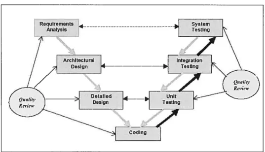
quality was treated as an afterthought or as a postscript in software development. Hilbum and Towhidnejad argued that software quality should be addressed in the front-end of the lifecycle and should not be ignored until after the development of the product [35]. They suggested that quality should be focused on dunng the whole software development process. figure 2.1 developed by Hilbum and Towhidnejad, shows a V Quality mode! that provides a conceptual framework for such a focus.

Figure2.1 The V Model for Quality

During the test phase, only the functional requirement can be determined. Aside from the functional requirement, there are other requirements; such as, maintainability, reusability, reliability, and stability that need to be determined. Unfortunately, these cannot be determined through testing. As a consequence of this problem, software quality has been treated as an afterthought in the software development process. This solution does flot appear to adequately address the quality issue; therefore, a better possible solution may be to apply software prediction models to assure software quality during the development lifecycle [53].

Software prediction models address the evaluation of software quality during the software development life cycle. The prediction model, specified fora specific project, consists of a set of important quality characteristics. In general there are six

Chapter 2 11

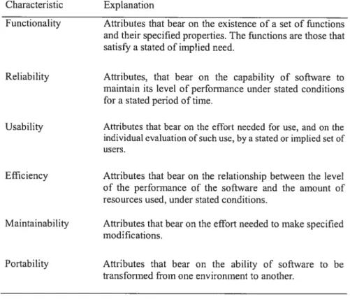
characteristics of software that can be used as criteria for quality as defrned in ISO/IEC 9126 (Sec Table 2.1).

Table 2.1 Software Characteristics from ISO/IEC 9216

Characteristic Explanation

Functionality Attributes that bear on the existence of a set of functions and their specified properties. The functions are those that satisfy a stated of irnplied need.

Reliability Attributes, that bear on the capability of software to maintain its level of performance under stated conditions for a stated period oftime.

Usability Attributes that bear on the effort needed for use, and on the individual evaluation of such use, by a stated or implied set of users.

Efficiency Affributes that bear on the relationship between the level of the performance of the software and the arnount of resources used, under stated conditions.

Maintainability Attributes that bear on the effort needed to make specified modifications.

Portability Attributes that bear on the ability of software to be transfonned from one environment to another.

2.3 Software Measurement and Metrics

Software measurement is another important concept that is concemed with deriving numeric values for some attributes of a software product or a software process. These values enable people to intuitively evaluate and draw conclusions about the quality of the software or the software process. Some large companies have introduced program metncs for measurement purposes and are using collected metrics in their quality management processes [56]. Most of the focus lias been on collecting metrics on the program and the processes of verification and validation. During the past decades, a lot of people (such as Offen, Jeffrey, Hall, and Fenton) have contributed for the introduction of software metncs as a way to improve software quality.

A software metric is any type ofmeasurement that relates to a software system, process

or related documentation [56]. For exampic, lines of code are the measurement of the

size of a software product. The fog index (Gunning, 1962) is a measure of the readability of a passage of written text. The number of reported faults in a delivered software product or the number of person-days required to develop a system component are also example of software metrics.

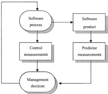
• Control Metrics and Predictor Metrics

There are two types of software metrics to consider: control metrics and predictor

metrics. Control metrics are usually associated with software processes (therefore they are also called process metrics by some researchers) whule predictor metrics are associated with software products. Examples of control (or process) mefrics are the average effort and time required to repair reported defects. Examples of prcdictor metrics include the cyclomatic complexity of a module, the average length of an identifier in a program, or the number of attributes and operations associated with objects in a design. Both control and predictor metrics may influence management decision making as shown in figure 2.2.

Chapter 2 13

• Dynamic Metrics and Static Metrics

Predictor metrics are concemed with characteristic ofthe software itself. Unfortunately, software characteristics, such as size and cyclomatic complexity that can be easily measured, do not have a clear and universal relationship with quality attributes such as understandability and maintainability. The relationships vary depending on the development process, technology and the type of system being developed. Organizations that are interested in software measurements have to construct a historical database, which can be used to discover how the software product attributes are related to the qualities of interest in the organization.

Product metrics fa!! into two classes:

1. Dynamic metrics, which are the co!!ected measurements made of a program in execution.

2. Static metrics, which are the co!lected measurements made of the system representations such as the design, program or documentation.

The two different types of metrics are re!ated to different qua!ity attributes. Dynamic metrics are to eva!uate the efficiency and the reliability of a program whereas static metrics are to evaluate the comp!exity, understandability and maintainabi!ity of a software system.

Dynamic metrics are usua!!y directly related to software qua!ity attributes. They are re!atively easy to measure. for examp!e, the execution time required for particu!ar functions and the time required to startup a system are dynamic metrics. These re!ate metrics directly to the system’s efficiency.

Static metrics, on the other hand, have an indirect re!ationship to quality attnbutes. There are a !arge number of these metrics proposed and experiments conducted to derive and validate the relationships between these metrics and system complexity, understandabi!ity and maintainabi!ity. Table 2.2 !ists several static metrics used for assessing qua!ity attributes. Among these, programlcomponent !ength and contro!

complexity seem to be the most reliable predictors of system understandability, complexity and maintainability [56].

Ail of the metrics in Table 2.2 are for function-oriented designs. Their usefulness as predictor metrics is stiil being established despite the increasing popularity of object-oriented software systems.

Table2.2 Function-Oriented Software Product Metrics Sofiware Description

Mefric

Fan-infFan- Fan-in is a measure of the number of functions that cali some out other function (say X). fan-out is the number of the functions which are called by function X. A high value for fan-in means that X is tightly coupled to the rest ofthe design and the changes to X wiII have extensive knock-on effects. A high value for fan-out suggests that overali complexity of X may be high because of the complexity of the control logic needed to coordinate the calledcomponents.

Length of This isa measure ofthe size ofa program. Generally, the larger code the size ofthe code ofa program component, the more complex

and etior-prone that compondnt is likely to be.

Cyclornatic This is a measure of the control cornplexity of a program. This complexity control complexity may be related to program

undcrstandability.

Length of This is a measure ofthc average length of distinct identifiers in a identiflers program. The longer the idcntiflers, the more likely they are to be meaningfiil and hence the more understandable the program. Depth of This is a measure of the depth of nesting of if-statements in a Conditional program. Deeply nested if-statements arc hard to understand

nesting and are potentially error-prone.

Fog index This is a measure ofthe average length ofwords and sentences in documents. The higher the value for the fog index, the more difficult the document may be to understand.

• Object-orïented Metrics

Since the early 1990s, there have been a number of studies conceming object-oriented metrics. Some of these were derived from the previously existing metrics shown in Table 2.2, but others are unique to object-onented systems. Table 2.3 explains some of the object-oriented metrics.

These specific metrics are dcpending on the project itseif, the goals of the quality management team and the type of software developed. In some situations, ail the

Chapter 2 15

metrics in Table 2.2.and Table 2.3 may be useful. However, there are situations where some metrics are inappropnate. Organizations should choose the most appropnate metrics for their needs.

Table 2.3 Object-oriented Metrics

Object-oriented Description Metric

Depth of This represents the number of discrete levels in the inheritance inheritance tree tree where subclasses inherit attributes and operations (methods) from superclasses. The deeper the inheritance tree, the more complex the design as, potentially, many different object classes have to be understood to understand the object classes at the leaves ofthe tree.

Method This is directly related to fan-in and fan-out as described in fan-inlfan-out Table2.2 and means essentially the same thing. However, it may be appropriate to make a distinction between calis from other methods within the object and cails from external method. Weighted This is the number ofmethods included in a class weighted by the rnethods cornplexity of each method. Therefore, a simple method may per class have a cornplexity of 1 and a large and complex method a mucb higher value. The larger the value for this metric, the more complex the object class. Complex objects are more likely to be more difficuit to understand. They may not be logically cohesive so cannot be reused effectively as superclasses in and inheritance tree.

Number of These are the number of operations in a superclass which are overriding ovenidden in a subclass. A high value for this metric indicates operations that the superclass used may not be an appropriate parent for

subclass

• Relations between Internai and External Attributes

Software quality characteristics are also categorized as internai or external by some

researchers. The size, inheritance, and coupling are internaI attributes and can be directly measured. While the external characteristics ofmaintainability, reusability, and reliability can only be measured after a certain time of use. In order to predict software quality characteristics, software attributes (or metrics) were introduced because their properties are directly measurable. Roughly speaking, building a software quality prediction model is akin to building a relationship between the measurable internai attributes and the external characteristics. Therefore, before talking about software quality prediction models, we also need to consider the measurable attributes of software and the software measurements which are introduced in the following.

Some software quaiity attributes (mostly the external attributes) are impossible to measure directiy. Attributes such as maintainability, complexity and understandability are affected by many different factors. There are no straightforward metrics for them. Therefore we have to measure some internai attribute of the software (such as its size) with the assumption that there is a reiationship bctween what we can measure and what we want to know. ldeaily, there should be a validated and clear relationship between the software extemal and internai attributes.

Figure 2.3 shows some external quality attributes that might be of interest [56]. On the diagram’s left side are some externai attributes and on the right side are some internai ones. This diagram shows that the measurable internai attributes might be reiated to the externai attributes. It suggests that there may be a reiationship between externai and internai attribtites but does not say what the relations are.

Chapter 2 17

If a measurement of an internai software attribute is to be a useftil predictor of an external one, three conditions must hold (Kithchenham, 99O):

1. The internai attribute must be measured accurately.

2. A reiationship must exist between the measurabie internai attnbute and the external behaviorai attribute.

3. This relationship is validated and can be expressed in terms of an understandable formula or mode!.

The mode! formulation invoives identifying the functionai form of the model (i.e. linear, exponential) by analyzing collected data and identifying the parameters which are to be included in the mode!. Such model development usually requires significant experience in statistical techniques if it is to be trnsted. A professional statistician should usually be involved in the process.

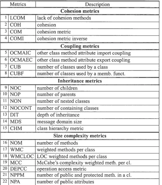
The software quality prediction models used in our study are based on the basic elernents ofa software measurement environment and the metrics described above. We choose 22 structural software metrics to predict its stability. The metrics (see Table 2.4) are grouped in four categories by coupling, cohesion, inheritance, and complexity. They constitute a union ofmetrics used in different theoretical models [17, 7, 59, 12].

After the software metrics are defined and collected, they can be used to buiid the relationship between the immeasurable software quaiities and the measurable software metrics. The assumed relations are called software quality prediction models.

Table 2.4 The 22 SoftwareMetncs Used as Attributes in Our Experiments

Metncs Description

Cohesion metrics 1 _{LCOM lack of cohesion methods}

2 _{COH cohcsion}

3 _{COM cohesion metric}

4 _{COMI cohesion metric inverse} Coupling metrics

5 _{OCMAIC other class method attribute import coupling} 6 _{OCMAEC other class method attribute export coupling} 7 CUB number of classes used by a class

8 CUBF number of classes used by a memb. funct. Inheritance metrics

9 NOC number of chiidren 10 _{NOP number of parents} 11 NON number of nested classes 12 NOCONT number of containing classes 13 DIT depth of inheritance

14 MDS message domain size 15 _{CHM class hierarchy metric}

Size complexity metrics

16 _{NOM number of methods}

17 WMC weighted methods per class 18 WMCLOC LOC weighted methods per class

19 _{MCC McCabe’s complexity weighted meth. per cl.} 20 DEPCC operation access metric

21 NPPM number of public and protected meth. in a cl. 22 _{NPA number of public attributes}

2.4 Software Quality Prediction Models and Building Approach

As mentioned before, software quality is evaluated in terms of maintainability,

reusability, reliability, stability, etc. The majority ofthese quality characteristics are not directly measurable. But we can use software metric values to help us estimate the software quality. b do this, we have to assume a relationship between them. Ibis is the software quality prediction (estimation) model.

Chapter 2 19

Software prediction models address the evaluation of software quality during the software development life cycle. The prediction model, specified for a specific project, consists of a set of important quality characteristics. These attributes (or metrics) are directly measurable software properties that qualify quality characteristics.

Software quality prediction models offer an interesting solution to assure software quality because they can be used to incorporate a wide variety of quality assurance techniques [53]. Most importantly, software quality prediction models can be used to predict the number of the defects (faults) in software systems before they are deployed

[24].

The approach to building software qtiality prediction models is very complex and source costing. Roughly speaking, building a quality prediction model consists of building a relationship between the intemal and extemal quality characteristics. There are a lot oftypical approaches to prediction models; such as, statistic, machine leaming, neural networking and BBN.

The work donc so far to build efficient and usable software quality prediction models falls into two families. The first one relies on historical measurement data to achieve its goal (sec for example [3], [14] and [43]). The quality of these models depends heavily on the quality of the samples used, which is usually poor in software engineering. lndeed, contrary to other domains, the small sizes and the heterogeneity ofthe samples makes it difficuit to derive widely applicable models. As a result, the models may capture trends, but do so by using sample-dependent threshold values [54]. Also, as stated by f enton & Neil [26], the majority of the produced models are naïve; they cannot serve as decision support during the software development process. This is because often the predictive variables and the quality characteristics used for prediction show no obvious causal link that could explain their derived relationship. The models

behave as simple black boxes that take the predictive variables as input and the predicted variables as output [53].

The second way of building software quality estimation models uses knowledge extracted from domain-specific heuristics. The obtained predictive models use judgments from experts to establish an intuitively acceptable causal relationship between internai software attributes and a quality characteristic. Although they are adapted to the thought decision-maldng process, these models are hard to generalize because of a lack of widely accepted common kriowledge in the field of software quality.

Consequently, there exists a need for an approach that combines the advantages of using both historical measurement data and domain 1uowledge.

2.5 Existing Software Quality Prediction Models

In fact, prediction models are becoming an efficient way to predict the quahty of the software at early stages of development. During the past decades, there have been a lot of studies and papers generated on this topic. Consequently, a large number ofproposed quality models have been proposed in the literature. There are many kinds of software quality prediction models. In this section we give an overview of four kinds of prediction models, whichfit in one ofthe following categones:

• Static Regression Models

• Bayesian Belief Networks Models • Neural Network Models

Chapter 2 21

2.5.1 Static Regression Software Defect Prediction Models

Most prediction models are based on size and complexity metrics. The earliest such models are typical of many regression based “data fitting” models which became common place in the literature. The resuits from regression rnethods showed that linear models of certain simple metrics provide reasonable estimates for the total number of defects D (the dependent variable is actually defined as the sum of the defects found during testing and the defects found dunng the two months after release). The following represcnts some regression equations posted in the literature:

D =4.$6+0.018L (1) D= V (2) 3,000 D —=A0+A1lnL+A-,lnL (3) D=4.2+0.0015(L)3”3 (4)

The first Equation (1) computed by Akiyarna [2], which was based on a system developed at fujitsti in Japan, predicted defects from lines of code (LOC). from (1) it can be calculated that a 1,000L (it is 1000 LOC) module is expected to have approximately 23 defects.

The second Equation (2) provided by Halstead [34] is a notable equation. This regression model predicts D, the number of defects, depends on a program F In this equation, V is the (language dependent) volume metric (which like aIl the Halstead metrics is defined in terms ofthe number of unique operators and unique operands in P; for details see [23]). The divisor 3,000 represents the mean number of mental discriminations between decisions made by the programmer.

computing V directly by using unes of executable code L instead. Specifically, he used the Halstead theory to compute a series ofequations. In equation (3), each ofthe Ai is dependent on the average number of usages of operators and operands per LOC for a particular language. For example, for Fortran A0 0.0047; A 0.0023; A, =0.000043.

For an assembly language n A0 =0.0012; i ‘O.0OO]; 112 =0.000002.

Gaffney [31], argued that the relationship between D and L was flot language dependent. In Equation (4), he used Lipow’s own data to deduce this prediction model. An

interesting ramification of this was that there was an optimal size for individual modules with respect to defect density. For (4) this optimum module size is $77 LOC.

Numerous other researchers have since reported on optimal module sizes. For example, Compton and Withrow of UNISYS derived the following polynomial equation, [19]:

D=0.069+0.00156L+0.00000047(L)2 (5)

Based on (5) and further analysis Compton and Withrow concluded that the optimum size for an Ada module, with respect to minimizing error density, is $3 source statements.

The realization that size-based metrics alone are poor general predictors of defect density spuned on much research into more discriminating complexity metrics. McCabe’s cyclomatic complexity, [45], has been used in many studies, but it too is essentially a size measure (being equal to the number of decisions plus one in most programs). Kitchenham et al. [40], examined the relationship between the changes experienced by two subsystems and a number ofmetrics, including McCabe’s metnc. Two different regression equations resulted in (6) and (7):

C =0.042MC1—0.075N+0.00001HE (6)

C —0.25MC1—0.53D1+0.O9VG (7)

For the first subsystem changes, C, was found to be reasonably dependent on machine code instructions, MCI, operator and operand totals, N, and Halstead’s effort metric,

Chaptei 2 23

HE. For the other subsystem McCabe’s complexity metric, VG was found to partially explain C along with machine code instructions, MCI and data items, Dl.

Ail of the metrics discussed so far are defined in terms of code. There are now a large number of metrics available earlier in the lifecycle of software, most of which have been claimcd by their proponents to have some predictive power with respect to residual defect density. for example, there have been numerous attempts to define metrics which can be extracted from design documents using counts of “between module complexity” sucli as cali statements and data flows; the most well known are the metrics in [49]. Ohisson and Alberg, [4], reported on a study at Ericsson where metrics derived autornatically from design documents were used to predict, in particular, fault-prone modules prior to testing. Recently, there have been several attempts, such as [17] and [19], to define metrics on object-oriented designs.

For the regression software defect prediction models, the essential problem is the oversimplification. Typically, the method is for a simple relationship between some predictor and the number of defects delivered. Size or complexity measures are often used as such predictors as mentioned above. The resuit is a naïve model.

Indeed, such models fail to include all the causal or explanatory variables needed to make the models generalizable. And they can only be used to explain a data set obtained in a specific context. In order to establish a causal relationship between two variables, Bayesian Belief Networks (BBN) was developed to improve the explanatory power.

2.5.2 Bayesian Belief Networks Models

The relationships between product, process attributes and numbers of defects may be too complex to apply straightforward curve fitting modeis. In predicting defects discovered in a particular project, additional variables can be added to the model, for

example, the number of defects discovered may depend on the effectiveness of the method with which the software is tested. it may also be dependent on the level of detail of the specifications from which the test cases are derived, the care with which requircments have been managed during product development, and 50 on. The BBN models are the better candidates for situations with such a rich causal structure.

A Bayesian BeliefNetwork(BBN) is a special type of diagram (called a graph) together with an associated set of probability tables. The graph is made up of nodes and arcs where the nodes represent uncertain variables and the arcs the causal/relevance relationships between the variables.

BBN model (also known as graphical probability models) use the subjective judgmcnts of experienced project managers to build the probability model. it can be used to produce forecasts about the software quality throughout the development life cycle. Moreover, the causal or influence structure ofthe model more naturally mirrors the real world sequence ofevents and relations that can be achieved with other formalisms.

The relationship between the attributes and the number of defects are too complex that additional variables, such as probability, have to be added to the model. Probability is a dynamic theory. It provides a mechanism for coherently revising the probabilities of events as evidence becomes available [28].

Fenton proposed a BBN mode! (see Figure 2.4) for an example “reliability prediction” problem in 1999[24]. We take his model and explanation to show the general

information of the BBN model.

In figure 2.4, the nodes represent discrete or continuous variables, for example, the node “use of IEC 1508” (the standard) is discrete having two values “yes” and “no,” whereas the node “reliability” might be continuous (such as the probability offailure). The arcs represent causal/influential relationships between variables. For example,

Chapter 2 25

software reliability is defined by the number of (latent) fauits and the operational usage (frequency with which faults may be triggered). Hence, this relationship was modeled by drawing arcs from the noUes “number of latent faults” and “operational usage” to “reiiability.”

NODE PROBABILITY TABLE (NPT) FOR THE NODE “RELIABILITY”

operational usage low med high

faults Iow rned high low rned high Iow rned high low 0.10 0.20 0.33 0.20 0.33 0.50 0.20 0.33 0.70 reliability med 0.20 0.30 0.33 0.30 0.33 0.30 0.30 0.33 0.20 high 0.70 0.50 0.33 0.50 0.33 0.20 0.50 0.33 0.10

Figure 2.4 “Reliabiiity Prediction” BNNExample

for the node “reiiabiiity” the node probabiiity table (NPT) might, therefore, look like that shown in the Figure 2.4 (for ultra-simplicity we have made ail nodes discrete so that

here reliability takes on just three discrete values low, medium, and high). The NPTs capture the conditional probabilities of a node given the state of its parent nodes. For nodes without parents (such as “use ofIEC 1508” in Figure 3.4) the NPTs are simply the marginal probabilities.

There may be several ways of determining the probabilities for the NPTs. One of the benefits of BBNs stems from the fact that we are able to accommodate both subjective probabilities (elicited from domain experts) and probabilities based on objective data. Recent tool developments mean that it is now possible to build very large BBNs with very large probability tables (including continuous node variables).

The most important advantages of using BBNs is the ability to represent and manipulate complex models that might neyer be implemented using conventional methods. Another advantage is that the model can predict events based on partial or uncertain data. Because BBNs have a rigorous, mathematical meaning there are software tools that can interpret them and perform the complex calculations needed in their use.

2.5.3 Neural Network Models

In the last decade, significant effort has been put into the research of developing prediction models using neural networks. Many researchers [Khoshgoftaar, 1995] realized the deficiencies of regression methods (see section 2.5.1) and explored neural networks as an alternative. Neural networks are based on the principle of learning from example and no pnor information is specified (unlike the Bayesian approach discussed in previous section). Neural networks are characterized in terms of three entities: the neurons, the interconnection structure and the leaming algorithm [Kamnanithi, 1992].

Neural networks are leaming-oriented techniques, which use prior and current knowledge to develop a software prediction model [39]. The multi-layer perception is

Chapter 2 27

the most widely applied neural network architecture today. Neurai Network Theory shows that only three layers of neurons are sufficient for leaming any (non) linear function combining input data to output data. The input layer consists ofone neuron for each complexity metric, while the output layer has one neuron for each quality metric to be predicted.

Because neural network based approaches are predominantly resuit-driven, flot dealing with design intuition or heuristic mies for modeling the development process and its products, and because their trained information is a black-box (that is to say, not accessible from outside). They are not suitable for providing the reasons for a particular resuit. Therefore, neural networks can be applied when only input vectors (software metric data) and results (quality or productivity data) are of concem, while no intuitive connections are needed between the two sets (e.g. pattem recognition approaches in complicated decision situations).

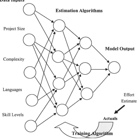
Most of the prediction models developed using neural networks use back-propagation feed-forward training networks (see Figure 2.5). The network is trained with a series of input and correct output from the training data so as to minimize the prediction error. Once the training is complete, and the appropriate weights for the network arcs have been determined, new input can be presented to the network to predict the corresponding estimate ofthe response variable.

Most of the models which developed using neural networks operate as “black boxes” and do not provide any information or reasoning about how the outputs are derived. It is hard to know whether the models satisfactorily predict software quality in different contexts or not.

Therefore we can see that neural networks cannot cunently provide any insight into why they arrived at a certain decision rather they only provide the resuit-driven

connection weights. It is interesting to note that feedforward fleurai nets can be approximated to any degree of accuracy by fuzzy expert systems [3$], hence offering a ncw approach for ciassification based on neurai ftizzy hybrids that can be trained and pre-popuiated with expert mies.

2.5.4 Decision Trec Models

Another kind of prediction modei is the decision trce model, aiso cailed a mie-based model. A decision tree modei is a kind of inductive modei that expiains the relationship

betwcen predictive and predicted variabies [57].

A decision tree aigonthm is attractive because of its expiicit representation of

Data Inputs Estimation A1%orithms Proj ect Mode! Output Languages Skiil Levels Effort Estirnate K, Actua!s

Chapter 2 29

classification as a series of binary spiits (sec Figure 2.6). A decision tree algonthm constmcts a tree, and the tree can also be translated into an equivaient set ofruies. Ibis makes the induced knowledge structure easy to understand and validate.

An empiricai decision tree represents a segmentation of the data that is created by appiying a series of simple mies. Each mie assigns an observation to a segment based on the value of oneinput. One mie is appiied afler another, resulting in a hierarchy of

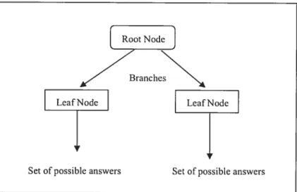
segments within segments. The hierarchy is caiied a tree, and each segment is called a node. The original segment contains the entire data set and is called the root node ofthe tree. A node with ail its successors forms a branch of the node that created it; the final nodes are called leaves. for each leaf, a decision is made and app]ied to ail observations in the leaf. The type of decision depends on the context. In predictive modeling, the decision is simply the predicted value.

Figure 2.6 A Decision Tree Diagram

In the decision tree:

• Each nonleaf node is connected to a test that spiits its set of possible answers into subsets con-esponding to different test results.

• Each branch carnes a particular test result’s subset to another node.

• Each node is coiruected to a set of possible answers. Root Node

BrancheN

A decision tree is a complete binarytree where each inner node represents a yes-or-no question, each edge is labeled by one ofthe answers, and terminal nodes contain one of the classification labels. The decision making process starts at the root of the tree. Given an input vector x, the questions in the internai nodes are answered, and the corresponding edges are followed. The label of x is detennined when a leaf is reached.

More specifically, decision trees classify instances by sorting them down the tree from the root node to some leaf nodes, which provides the classification of the instance. Each node in the tree specifies a test of some attribute of the instance, and each branch descending from that node corresponds to one of the possible values for this attribute.

An instance is classified by starting at the foot node of the decision tree, testing the attribute specified by this node, then moving down the tree branch corresponding to the value ofthe artribute. This process is then repeated at the node on this branch andso on until leafnode is reached.

A decision tree is induced from a table of individual cases, each of which describes identified attributes. At each node, the algorithm builds the tree by assessing the conditional probabilities linking attributes and outcomes, and divides the subset of cases under consideration into two further subsets so as to minimize entropy according to the cnterion it chooses. The cnterion for evaluating a splitting mie may be based on either a statistical significance test or on the reduction in variance or entropy. Ail criteria allow the creation ofa sequence ofsub-trees.

Normally, the decision tree is constructed by Quinlans 1D3 algonthm. C4.5 is a software extension of the basic 1D3 algorithm designed by Quinlan. This algonthm belongs to the ‘divide and conquer’ family of algorithms where a decision tree generally represents the induced knowledge.C4.5 works with a set ofexamples that has the same structure and consists of a number of attribute/vaiue pairs. One of these

Chapter 2 31

attributes represents the ciass of the example. Most of the time the ciass attributes are binary and take oniy the value {tme, faise}, or {success, failure}. The key step ofthe algorithm is selecting the “best” attnbute so as to obtain compact trees with high predictive accuracy.

An advantage of decision trec models over other modeis is that thisldndofmodei may represent interpretable English mies or logic statements. For example,

‘1f

inortgage-to-income ratio is less than 25% and months posted Ïate is tess

than

and

than

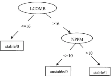
In generai, decision trees represent a disjunction of conjunctions of constraints on the attribute-values of instances. Each path from the tree root to a leaf corresponds to a conjunction of attribute tests, and the tree itself to a disjunction of these conjunctions. Our aigorithm is designed specificaliy to combine the classic-mie based prediction modeis for stabiiity into one final classifier. A ciassic-nile based prediction modeis is a set ofdecision tree ciassifiers (Figure 2.7).

/

/

r

The following example provides a sample rule that is derived from the above decision tree.

LCOMB> 16

NFFM<= 10

— class 0 [63.0%]

Figure 2.8 A Rule Set Translated from figure 2.7

2.6 Summary of this Chapter

in this chapter we described the basic concepts of software quality. We also introduced the main approaches of building software quality prediction models and some of the existing models. in our research, we will propose a new method —a combination algorithm by using a genetic algorithm—to build new models. We use existing decision

tree models (mie based models) as our input and we believe the obtained new models have better prediction ability. in the next chapter we will describe the genetic aigorithm in more detail.

Cliapter 3

Genetic Algorithm Principles

A genetic algorithm (GA) is an optimization tecimique that was introduced in the late 60’s by John Holland [36J. GAs were inspired by Darwin’s theory of evolution. They can be used for applications such as training neural networks, setecting optimal regression models and discriminant (pattern recognition) optimization [22].

A GA imitates the process ofcreating a new population ofindividuals. The components ofa GA are chromosomes each of which display a certain fitness. The fitness is used to measure how wetl the individual perforrns in its environment. The key idea of the Darwinian theoiy of evolution is that new chromosomes are created and the fittest remain until the end and propagate their genetic material during evolution. The new chromosomes are created through three major operators: selection, crossover/recombination and mutation [22].

In this chapter, we first give a brief introduction to the GA. Then we describe GA concepts: operators and parameters. finatty we present the GA application.

3.1 Introduction of Genetic Algorithm Principles

The scope ofGAs is very broad. GAs are a part ofevolutionary computing, which is a rapidly growing technique ofartificial intelligence [51]. Generally, the process ofa GA can be described as follows:

A GA starts with a set of solutions (represented by chromosomes) called the original population. Solutions from the original population are taken and used to form a new population. lt is hoped that the new population will be better than the old one. Solutions selected to forrn new solutions (offspring) are chosen according to their fltness. The more suitable they are the more chances they have to reproduce. This process of reproduction is repeated until certain conditions, for example, the number of generations or the best solution, are satisfied.

The following represents the outline process of a typical GA.

L IStarti Generate a random population ofnchromosomes (suitable solutions for

the problem).

2. tfitnessl Evaluate the fitnessf(r) ofeach chromosome x in the population. 3. tNew populationJ Create a new population by repeating the following steps

until the new population is complete.

1. tSelectionl Select two parent chromosomes from a population according to their fitness (the better the fitness, the better the chance of being selected).

2. ICrossoveri Using crossover probability, cross over the parents to forni new offspring (chiidren). 1f no crossover is performed, offspring is an exact copy of the parents.

3.

tMutationl

4.

tAcceptingi

4. tReplacel Use newly generated population for a furtherrunof the algorithm.

5. tTestl If the end condition is satisfied,

stop,

current population. 6. tLoopl Go to step 2.

This outiine of the GA process is only a general one. There are many things that can be implemented in different ways and in various domains.

In

Chapter 3 35

3.2 Terms of Genetic Algorïthm

Before going into the details of a GA, some terms associated with it nced to be defined to help understand how it works.

3.2.1 Chromosome, Gene and Genome

From the view of biology, ail living organisms consist of ceils. Each ccli contains the same set of chromosomes. Chromosomes are strings ofDNAand serve as amodel for the whole organism. A chromosome consists of genes that are blocks of DNA. Each gene encodes a particular protein and a trait such as the color ofeyes. Possible settings for a trait (e.g. blue, brown) are called alleles. Each gene has its own position in the chromosome. The position ofa gene is called its locus. The genome is the completc set of genetic material (ail chromosomes).

GA borrowed several terms from biology. For example, the term chromosome refers to one individual element in the search space. A chromosome is formed from genes. Simply speaking, genes are the individual instructions that teli the organism how to develop and keep the body healthy, while chromosomes are the structures that hold the genes. In every ccli of an organism there are thousands of genes that are located on each chromosome. Chromosomes occur as pairs. f igure 3.1 shows a pair of chromosomes and a chromosome structure.