HAL Id: hal-01879573
https://hal.archives-ouvertes.fr/hal-01879573
Submitted on 24 Sep 2018
HAL is a multi-disciplinary open access
archive for the deposit and dissemination of sci-entific research documents, whether they are pub-lished or not. The documents may come from teaching and research institutions in France or abroad, or from public or private research centers.
L’archive ouverte pluridisciplinaire HAL, est destinée au dépôt et à la diffusion de documents scientifiques de niveau recherche, publiés ou non, émanant des établissements d’enseignement et de recherche français ou étrangers, des laboratoires publics ou privés.
Dynamic Modeling of Heat Transport in District
Heating Networks
Manuel Betancourt Schwarz, Bruno Lacarrière, Carlos Santos Silva, Pierrick
Haurant, Mohamed Mabrouk
To cite this version:
Manuel Betancourt Schwarz, Bruno Lacarrière, Carlos Santos Silva, Pierrick Haurant, Mohamed Mabrouk. Dynamic Modeling of Heat Transport in District Heating Networks. ECOS 2018 - 31st International Conference on Efficiency, Cost, Optimization, Simulation and Environmental Impact of Energy Systems, Jun 2018, Guimaraes, Portugal. �hal-01879573�
Dynamic Modeling of Heat Transport in District
Heating Networks
Manuel Betancourt Schwarza, Bruno Lacarrièreb, Carlos Santos Silvac, Pierrick
Haurantd and Mohamed Tahar Mabrouke
a IMT Atlantique – IST de Lisboa, Nantes, France, manuel.betancourt-schwarz@imt-atlantique .fr, b IMT Atlantique, Nantes, France, bruno.lacarriere@imt-atlantique.fr
c IST de Lisboa, Lisbon, Portugal, carlos.santos.silva@tecnico.ulisboa.pt d IMT Atlantique, Nantes, France, Pierrick.HAURANT@imt-atlantique.fr e IMT Atlantique, Nantes, France, mohamed-tahar.mabrouk@imt-atlantique.fr
Abstract:
District Heating (DH) networks are getting closer and closer to the concept of “Smart Grids” to deal with the contribution of new technologies and paradigms like Renewable Energy Sources, Distributed Generation, Low Energy Buildings, Distributed Storage and Low Temperature District Heating. This requires good anticipation of the system’s dynamics with the objective of improving control, which is of less importance in classical DH. This work analyses the specificities of DH for anticipating this dynamics and a simulation model for the heat transportation in a network is proposed, based on a finite element transient model. Its application to branched network topologies gives the spatio-temporal distribution of temperature along all the pipes and in all the network’s nodes within a specified time frame, regardless of the number of input and output pipes in the node. With it we can see the delay between the change in the settings at the generation points and the time they are perceived by the different substation in the network, which is a prerequisite for optimal control. The model is tested using different inputs that are forced to vary greatly to highlight the results. A comparison between the model developed by the authors and the existing Node method is presented. These results shed light on the necessities and opportunities in DH, mainly for enhanced control in the new energy context.
Keywords:
District Heating, Smart Thermal Networks, Transient Modeling.
1. Introduction
District Heating (DH) is a system that supplies heat to different users connected to centralized or distributed heat generation units through a pipe network, these systems can be as large as a complete city. DH has long been considered to be static, operative control is kept to a minimum and the network is reconfigured only occasionally [1,2]. This model of design and operation is proving to be outdated. The incursion of Renewable Energy Sources, Distributed Generation, Low Energy Buildings, Distributed Storage and the possibility of Low Temperature District Heating, among others, is demanding a change in the way we plan and operate DH. This change could come in the way of Smart Thermal Networks [3].
Smart Networks (SN) are a relatively new concept that gained international attention when the electricity sector started applying them in what we now call Smart Grids [4]. Even with their current popularity, they are not yet completely defined, but most authors [5–8] agree that SN are systems capable of: 1) making automated decisions concerning the current and future status of the network to guarantee its expected operation and 2) integrating all users connected to it and enabling them to participate actively in the activities of the network; this with the overall objective of higher efficiencies (economic and technical) and sustainability while maintaining the Quality of Service (QoS).
In the future, District Heating is expected to connect low energy buildings through low temperature networks with increased efficiency where renewable energies and distributed generation are smoothly integrated [9]. These systems will be economically and environmentally sustainable. To
do so, DH will rely heavily on Communication and Control infrastructures. In analogy with Electric Smart-Grids, Smart Thermal Networks will depend on Information and Communication Technologies (ICTs) for quality monitoring, timely information exchange and effective control [10].
Because instrumenting existing DH networks for research activities can be very costly and positive results are not guaranteed, a different way for assessing the impact of technological and operational changes has been pursued in the form of Modeling and Simulation (M&S) [11–14]. With M&S it is possible to replicate existing DH systems and modify them virtually to evaluate the possible results without incurring in high costs.
With the objective of using M&S to assess the impact that ICTs would have in turning DH into Smart Thermal Networks, this paper presents a model developed to simulate the dynamic response of branched DH systems to changes in Generation, Supply and/or Demand. In this paper the physical and mathematical basis is explained and emphasis is made on how the model is capable of performing accurately even when the temperature and the mass flow rate vary greatly, suddenly and/or constantly in time. This model will allow the incorporation of monitoring, communication and control strategies to evaluate the energy and economic performance of DH as Smart Thermal Networks in future work.
2. Methodology
DH can be represented as a web of interconnected nodes [15], where generation and consumption spots are the nodes, and the vertices connecting them are the buried-underground supply and return pipes transporting the water. For this reason the model is composed of two sub-models, one representing the vertices and another one the nodes. The response to the change of the inputs or outputs is expressed as a spatial-temporal distribution of temperatures and mass flow rates in the system.
The sub-model representing the pipes, namely the Heat Transport sub-model, is modeled on the physical phenomena of Mass Transport and Heat Transfer in a pipe and is based on the existing Node method [11,15] but coupled with the electrical analogy for thermal systems to calculate the inertia and the losses [16]. A comparison between this Modified method and the Node method will be presented. The sub-model representing the network, namely the Distribution sub-model, uses oriented graphs in combination with energy and mass conservation equations, head loss calculation and time series. Together they evaluate the direction, attenuation, delay and damping of the heat train across the network.
In order to make the simulations less computational intensive, the following considerations are made:
▪ Flow is one-dimensional and incompressible; ▪ Axial conduction and heat dissipation are ignored;
▪ The specific heat at constant pressure (𝐶𝑝) is constant in the evaluated range;
▪ Each element of the discretized pipe has a lumped mass with a single temperature (see Fig. 1); ▪ Heat inertia of insulation and ground are ignored.
These considerations are similar to those taken in other works which report accurate results for the modeling of thermal networks [11,15,17]. Both models are further explained in the following sections.
Fig. 1: Diagram of discretized pipe. j indicates the pipe element in the spatial discretization and Δx its length; T are the temperatures; 𝑚̇ is the mass flow rate of the water; and Q are the heat flows.
2.1. Heat Transport sub-model
The Heat Transport sub-model derives from the enthalpy balance for the energy flows in a discretized pipe. The energy flow, or heat flow, has two main components: 1) The axial component, or transported heat, which is the heat carried by the water along the pipe, and 2) The radial component, or transferred heat, which is the heat that the water loses through the walls of the pipe. Every pipe element has three associated heat flows that determine the change in its stored energy (∆𝑄𝑣𝑜𝑙), two for the axial component and one for the radial. On the axial axis there are the heat that
flows in from the upstream element (𝑄𝑖𝑛), dependent on the mass flow rate and the temperature the
water had when it left the previous element, and the heat that is passed to the downstream element (𝑄𝑜𝑢𝑡), dependent on the mass flow rate and the temperature the water had when it exited the analyzed element. On the radial axis there is the heat that is lost through heat transfer during the time the water is in the evaluated element (𝑄𝑝𝑒𝑟𝑑), this heat depends on the difference in temperatures between the pipe wall and the water. The enthalpy balance for an element 𝒋 of the pipe at time 𝒊 is shown in (1). 𝑄𝑖𝑛𝑖 𝑗 − 𝑄𝑜𝑢𝑡𝑗 𝑖 − 𝑄 𝑝𝑒𝑟𝑑𝑗 𝑖 = ∆𝑄 𝑣𝑜𝑙𝑗 𝑖 (1)
The balance in (1) can be expressed using the two variables for the system: the mass flow rate (𝑚̇) and the temperature (𝑇𝑤) of the water. In explicit form, these can be seen in (2).
𝑄𝑖𝑛𝑖 𝑗 = 𝑚̇𝑖𝐶𝑝𝑤𝑇𝑤𝑗−1 𝑖−1∆𝑡 𝑄𝑜𝑢𝑡𝑖 𝑗 = 𝑚̇𝑖𝐶𝑝𝑤𝑇𝑤𝑗 𝑖−1∆𝑡 𝑄𝑝𝑒𝑟𝑑𝑖 𝑗 =(𝑇𝑤𝑗−1 𝑖−1 −𝑇 𝑠𝑡𝑗𝑖 ) 𝑅𝑤−𝑠𝑡 ∆𝑡 ∆𝑄𝑣𝑜𝑙𝑖 𝑗 = 𝜌𝑤𝐶𝑝𝑤𝑉𝑤(𝑇𝑤𝑖𝑗− 𝑇 𝑤𝑗 𝑖−1) (2)
To be able to solve the enthalpy balance it is necessary to know the temperature of the steel (𝑇𝑠𝑡𝑖𝑗) in order to calculate the losses. In the Node method a second enthalpy balance is made for the steel pipe as shown in (3). In this case the change of the energy in the steel pipe is caused by the heat transferred from the water to the pipe (first item in bracket) and the heat transferred from the pipe to the environment (second item in bracket). 𝑇𝑎𝑗
𝑖 is the ambient temperature and 𝑅
𝑠𝑡−𝑎 is the resistance
between the steel pipe and the surroundings (including insulation resistance and soil resistance) 𝜌𝑠𝑡𝐶𝑝𝑠𝑡𝑉𝑠𝑡(𝑇𝑠𝑡𝑗 𝑖 − 𝑇 𝑠𝑡𝑗 𝑖−1) = [(𝑇𝑤𝑗 𝑖 −𝑇 𝑠𝑡𝑖) 𝑅𝑤−𝑠𝑡 − (𝑇𝑠𝑡𝑗𝑖 −𝑇𝑎𝑗𝑖 ) 𝑅𝑠𝑡−𝑎 ] [∆𝑡] (3)
Equations (1) and (3) create the 𝐴𝑥 = 𝐵 matrix system shown in (4) which can be solved by 𝑥 = 𝐴−1𝐵 .
[ 𝜌𝑤𝐶𝑝𝑤𝑉𝑤 ∆𝑡 + 1 𝑅𝑤−𝑠𝑡 −1 𝑅𝑤−𝑠𝑡 −1 𝑅𝑤−𝑠𝑡 𝜌𝑠𝑡𝐶𝑝𝑠𝑡𝑉𝑠𝑡 ∆𝑡 + 1 𝑅𝑤−𝑠𝑡+ 1 𝑅𝑠𝑡−𝑎 ] [ 𝑇𝑤𝑖𝑗 𝑇𝑠𝑡𝑖 ] = [ 𝑚̇𝐶𝑝𝑤𝑇𝑤𝑖−1𝑗−1+ ( 𝜌𝑤𝑉𝑤 ∆𝑡 − 𝑚̇) 𝐶𝑝𝑤𝑇𝑤𝑗 𝑖−1 𝜌𝑠𝑡𝐶𝑝𝑠𝑡𝑉𝑠𝑡 ∆𝑡 𝑇𝑠𝑡𝑗 𝑖−1+ 𝑇𝑎𝑗 𝑖 𝑅𝑠𝑡−𝑎 ] (4)
In the Modified method here presented, 𝑇𝑠𝑡𝑖𝑗 is obtained using the electrical analogy of the system. The electrical analogy transforms the thermal conductivities into electrical resistances, the heat capacities into electrical capacitances and the temperature gradients into voltages; the system can then be solved as an RC circuit. The converted circuit for a pipe like the one shown in Fig. 1 is shown in Fig. 2:
Fig.2: Thermal Circuit for an insulated pipe considering only one capacitance.
In Fig. 2, 𝑇𝑤 is the temperature of the water, 𝑇2 is the temperature of the interface between pipe and water, 𝑇𝑠𝑡 is the temperature at the middle of the steel pipe, 𝑇4 is the temperature at the interface between steel and insulation, 𝑇5 is the interface between insulation and the soil and 𝑇𝑎 is the ambient temperature. 𝑅1 is the thermal resistance of the water obtained from the convective heat transfer coefficient of the water and the area of contact between water and steel, 𝑅2 is half the thermal resistance of the steel pipe, 𝑅3 is the other half of this resistance, 𝑅4 is the thermal resistance of the insulation and 𝑅5 is the thermal resistance of the soil. 𝐶𝑠𝑡 is the heat capacitance of
the steel pipe and is equal to: 𝐶𝑠𝑡 = 𝜌𝑠𝑡𝐶𝑝𝑠𝑡𝑉𝑠𝑡 [18]. 𝑅2, 𝑅3 and 𝑅4 are calculated using the
resistance equivalent for a cylindrical geometry and 𝑅5 using the shape factor for a constant
temperature cylinder buried in a half infinite domain [16].
The solution for the circuit in Fig. 2 for the change from time step 𝑖 − 1 to time step 𝑖 can be found using the Laplace transform of the system as it eases the math [19]. Using 𝑇𝑠𝑡𝑗
𝑖−1 as reference
temperature for this change the resulting equation can be seen in (5). In this case 𝑅𝑤−𝑠𝑡 is the resistance between the water and the middle of the pipe (𝑅1+ 𝑅2) and 𝑅𝑠𝑡−𝑎 is the resistance between the middle of the pipe and the surroundings (𝑅3 + 𝑅4+ 𝑅5).
𝑇𝑠𝑡𝑖𝑗 = 𝑇 𝑠𝑡𝑗 𝑖−1+ {[𝑇 𝑤𝑗−1 𝑖−1 − 𝑇 𝑠𝑡𝑗 𝑖−1] [( 1 𝑅𝑤−𝑠𝑡𝐶𝑠𝑡) 𝑒𝑥𝑝 (− ( 𝑅𝑤−𝑠𝑡+𝑅𝑠𝑡−𝑎 𝑅𝑤−𝑠𝑡∙𝑅𝑠𝑡−𝑎∙𝐶𝑠𝑡) ∆𝑡)]} {∆𝑡} (5)
Equation (5) allows expressing the temperature of the steel pipe in function of the temperature of the water coming into the volume. Because all the temperatures at time 𝑖 − 1 are known from previous calculations, with the Modified method it is now possible to solve the enthalpy balance for 𝑇𝑤𝑗 𝑖 (6). Where 𝑇 𝑠𝑡𝑗 𝑖 is calculated with (5). 𝑇𝑤𝑖𝑗 =𝑚̇𝐶𝑝𝑤𝑇𝑤𝑗−1 𝑖−1 ∆𝑡+(𝜌 𝑤𝑉𝑤−𝑚̇∆𝑡)𝐶𝑝𝑤𝑇𝑤𝑗𝑖−1−(𝑇𝑤𝑗−1 𝑖−1 −𝑇𝑠𝑡𝑖 𝑗) 𝑅𝑤−𝑠𝑡 ∆𝑡 𝜌𝑤𝐶𝑝𝑤𝑉𝑤 (6)
Equations (4) and (6) remain true if the volume of the water evaluated in one element is equal or greater than the volume of the mass flow rate of water entering the element. This constraint is known as the Courant-Friedrich-Levy condition (𝐶𝐹𝐿 =𝑢∙∆𝑡
∆𝑥 ≤ 1). If the CFL is not met the system
presents instability; if the CFL is lower than 1 the system presents numerical diffusion. In systems with transient conditions and varying mass flow rates (varying 𝑢), trying to keep a CFL equal or close to 1 can be very computational intensive. Approaches that allow for accurate results for a higher range of mass flow rates without increasing computational time are preferred.
2.2. Distribution sub-model
The modeling of the DH network is done through the use of oriented graphs. Every edge of the graph corresponds to a pipe with the associated characteristics pertaining to it (length, diameter, material, insulation, etc.). Every node of the oriented graph corresponds to a node of the network (i.e. substations, junctions or splits) and it contains the information regarding to local generation, consumption or storage in the form of equations or time series. The graph transforms the physical connection of the network into a matrix called the Adjacency Matrix.
The characteristics associated to the edges are uploaded from a data base of various DH pipes. In the case of a split, where the in-flow divides itself into any number of out-flows, the Darcy-Weissbach equation for head loss (5) is used in combination with an optimization algorithm to calculate the mass flow through each edge. In (5), DW is the head loss, 𝐿 is the length of the pipe, 𝑢 is the speed of the flow, 𝑔 is the gravity, 𝑑 is the diameter of the pipe and 𝑓 is the friction factor. This last can be calculated using the explicit equation introduced by Barr in 1975 (6) [20], which provides accurate results for Reynolds numbers higher than 105. In (6) 𝑒𝑠 is the effective roughness
and Re is the Reynolds’ number. 𝐷𝑊 =4𝑓𝐿𝑢2 2𝑔𝑑 (5) 𝑓 = 1 [−4𝑙𝑜𝑔10(3.71𝑑𝑒𝑠 + 5.1286 𝑅𝑒0.89)] 2 (6)
To find how the flow distributes itself through the various outputs, the least squares optimization algorithm is used to find the values of u that will balance the pressure drop among all the output pipes while satisfying the conservation of mass.
Once this is done the next step is to model the processes at the different nodes. Fig. 3 shows a node (substation node) with its flows, in this figure we can see that a node with no generation has 5 mass flow rates and 5 temperatures that have to be determined (6 temperatures in the case of a node with generation):
1. One temperature (𝑇𝑠) (𝑇𝑠𝑖𝑛 and 𝑇𝑠𝑜𝑢𝑡 in the case of node with generation) and two mass flow
rates (𝑚̇𝑠𝑖𝑛 ; 𝑚̇𝑠𝑜𝑢𝑡) at the supply line.
2. Two temperatures (𝑇𝑅𝑖𝑛 ; 𝑇𝑅𝑜𝑢𝑡) and two mass flow rates (𝑚̇𝑅𝑖𝑛 ; 𝑚̇𝑅𝑜𝑢𝑡) at the return line.
3. Two temperatures (𝑇𝑠𝑢𝑏𝑖𝑛 ; 𝑇𝑠𝑢𝑏𝑜𝑢𝑡) and one mass flow rate (𝑚̇𝑠𝑢𝑏) at the heat exchanger.
Fig. 3: Example of a Node found and its flows in a DH system.
The input mass flow rates and temperatures for the supply and return lines depend on their upstream nodes. The temperature and mass flow rates at the heat exchanger of the substation can be obtained if we know the demand (𝑄𝐷𝑘) and the heat exchangers efficiency (𝜂𝑘) (calculating the heat
exchangers efficiency is outside the scope of this work). The output mass flow rates and temperatures of the supply and return lines can be calculated once we know their input temperatures and mass flows and the mass flow of the heat exchanger.
It is possible to see that most of the data needed for the balance at the nodes is obtained from the Distribution Model. The only values that are not from this model are 𝑇𝑠 and 𝑇𝑅𝑖𝑛. To obtain these
values we need to couple the two models together.
2.2. The coupled model
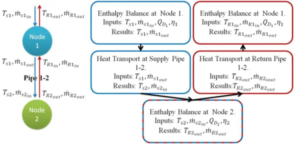
The two sub models work together to represent the DH network. The Distribution sub-model recreates the topology and the node dynamics (generation, consumption, storage) and the Heat Transport sub-model simulates the transport phenomena and the heat losses. An example of how the sub-models work together can be seen in Fig. 4. In this example two nodes are analysed with Node 2 being an end of the line node. The temperatures and mass flow rates are calculated for every time 𝑖. The result supply temperatures and mass flow rates from Node 1 are fed into the supply Pipe 1-2, the results from this pipe are fed into Node 2. Because Node 2 is at the end of the line, its results are fed to the return Pipe 1-2, which in turn are fed into Node 1. This process is repeated for any number of nodes, always starting at the first upstream nodes for the supply line and at the last downstream nodes for the return line.
Fig 4: Diagram of the coupled model for two nodes. Node 2 is an end of the line node.
Because 𝑇𝑠𝑢𝑏
𝑜𝑢𝑡𝑘 is fixed in these simulations, the network will present variable mass flow rates and
temperatures in the output pipes of the nodes, even if the mass flow rate at their input is constant. To guarantee the robustness of the model we calculate the CFL for all the pipes at every time interval and change the spatial discretization if it falls out of the accepted values.
3. Case Studies
The model was assessed with two different case studies. In the first, the output temperature of a single supply pipe connecting two nodes was tested for startup conditions simulated as a square input and a pipe full of cold water. The characteristics of the pipe can be seen in Table 1; ∅ is the pipe diameter, 𝑠𝑠𝑡 is the pipe thickness and 𝑠𝑖𝑛𝑠 is the insulation thickness.
Table 1. Characteristic of the Pipe used in the Single Pipe simulation.
Length 𝑚̇ ∅ 𝑠𝑠𝑡 𝑠𝑖𝑛𝑠 𝑧𝑑𝑒𝑝𝑡ℎ 𝑘𝑠𝑡 𝑘𝑖𝑛𝑠 𝑘𝑠𝑜𝑖𝑙 𝜌𝑠𝑡 𝐶𝑝𝑠𝑡 (𝑚) (𝑘𝑔 ∙ 𝑠−1) (𝑚𝑚) (𝑚) (𝑊 ∙ 𝑚−1∙ 𝐾−1) (𝑘𝑔 ∙ 𝑚−3) (𝐽 ∙ 𝑘𝑔−1∙ 𝐾−1)
Pipe 2000 8 90 10 53 1 54 0.024 1.2 7850 465
The second case study simulated a branched network composed of 6 nodes. The topology of this system is shown in Fig. 5 and the pipe characteristics in Table 2. This topology is the simplest most representative of a branched network as it includes the three main types of node connections found in a real network: 1) One upstream node feeding one downstream node; 2) Two or more upstream nodes feeding a downstream node; and 3) One upstream node feeding two or more downstream nodes.
Fig 5: Oriented Graph for the 6 node branched network used for the case study simulations. Table 2. Characteristics of the Pipes used in the Network Simulation.
Pipe Length 𝑚̇ ∅ 𝑠𝑠𝑡 𝑠𝑖𝑛𝑠 𝑧𝑑𝑒𝑝𝑡ℎ 𝑘𝑠𝑡 𝑘𝑖𝑛𝑠 𝑘𝑠𝑜𝑖𝑙 𝜌𝑠𝑡 𝐶𝑝𝑠𝑡 (𝑚) (𝑘𝑔 ∙ 𝑠−1) (𝑚𝑚) (𝑚) (𝑊 ∙ 𝑚−1∙ 𝐾−1) (𝑘𝑔 ∙ 𝑚−3) (𝐽 ∙ 𝑘𝑔−1∙ 𝐾−1) 1,3 1000 15 114.6 12.7 31 1 54 0.024 1.2 7850 465 2,3 1200 12 102.2 11.4 29 1 54 0.024 1.2 7850 465 3,4 750 27 73.6 8.2 36.5 1 54 0.024 1.2 7850 465 3,5 800 9.24 90 10 26.5 1 54 0.024 1.2 7850 465 5,6 800 17.76 90 10 26.5 1 54 0.024 1.2 7850 465
In this example Nodes 1 and 2 are generation nodes with no consumption, and Nodes 3, 4, 5 and 6 are Middle nodes with consumption, the network is considered to extend beyond Nodes 4 and 6 but it is not farther analyzed. The simulation starts after a time when the DH system was allowed to reach a cold state. Node 1 starts injecting energy into the network represented by a square pulse of the temperature from the beginning and Node 2 forty minutes later as a step reaching a constant temperature. The rest of the nodes start taking energy from the network 50 minutes after generation in Node 1 starts. The mass flows in Table 2 are the initial flows, before consumption starts.
4. Results
The results for the two case studies are presented in this section. For the single pipe case the results show the comparison between the Node method and the Modified method. The results from both methods are compared for different CFL values and time steps.
The results for the six node network using the modified are later presented. For this case study the results show the spatial-temporal distribution of the temperatures and powers in each of the six nodes together with the mass flow rates and their variation in time.
4.1. Single Pipe Test
The results for the first case study using a time step of 2.5 s are shown in Fig. 6; in 6a, the red line represents the square input at the beginning of the pipe, the blue line is the output calculated using the Modified method and the green line is the output calculated using the Node method. This figure shows that for CFL=1 the difference between both methods cannot be noticed. It can also be seen that the temperature signal at the output is: 1) delayed 38 min due to the length and the thermal inertia of the pipe; 2) attenuated up to 2°C because of the losses the flow suffers in its path, and 3) dampened by the thermal inertia of the steel in the DH pipe (the square input becomes an undulating output).
(a)
(b) (c)
Fig. 6: a) Temperature output calculated using the two different methods. b) Temperature output calculated with the Modified method for different CFL values. c) Temperature output calculated with the Node method for different CFL values.
Figs. 6b and 6c show the output for the same input but for different CFL values, it can be seen that lower CFL values tend to overestimate the time of arrival of the Heat Train and then underestimate the time it takes for the system to reach its maximum power; the lower the value of CFL, the greater the error. In Fig. 6b a CFL value of 0.2 overestimates the arrival by 0.5 min and underestimates the time to max power by 1.0 min. In Fig. 6c a CFL value of 0.2 overestimates the arrival by 1.0 min and underestimates the time to max power by 2.0 min. Both methods take similar computing times but it can be observed that with the modified method the results show less sensitivity to the CFL value. The modified method allows for more robust calculations on systems with varying mass flow rates when the spatial and temporal discretization remain fixed to prevent high computational times.
4.3. Six Node Network Test
After the modified method was tested for a single pipe, a more complex network was simulated. This case study evaluates a network that contains joints and splits and presents variable temperatures and mass flow rates. The results from this fluctuating system are shown in Figs. 7 to 9. In Fig. 7 it can be seen how the supply temperature signal is delayed by 19 min in Node 3, 28 min in Node 4, 26.5 min in Node 5 and 34 min in Node 6. Fig. 8 presents the mass flows, constant
during no-consumption times and varying once it starts at t=60 min. Fig. 9 shows how the nominal power takes some time to be available at every node and how the available power varies for each node once consumption starts.
Fig. 7: Supply temperature distribution for the network simulated network.
Fig. 8: Supply mass flow rate at the output of every node in the simulated network.
Fig. 9: Available power at every node for the simulated network.
From Fig. 7 it can be noticed that the heat train takes different times to arrive at the different nodes and that at any given moment the temperature is not the same along the network, it also comes to view that consumption does not affect much the temperature of the nodes. Nevertheless, consumption does affect the mass flow rates and its impact can be seen in Fig. 8. In this figure it is observed how, once consumption starts around t=60 min, the mass flow to the downstream nodes decreases. For this simulation consumption is considered to start instantly, which causes the steep drop in the mass flow rate that comes out from a node. The impact of the results from Fig. 7 and Fig. 8 together can be seen in Fig 9, where the power available at every node is plotted.
In Fig. 9 the power oscillates in time depending on the temperature and the mass flow. The different profiles that the curves belonging to each node have accentuate the complexity that DH systems face. Even when the temperature and mass flows at the input nodes is known and time series exist to estimate the consumption at the middle nodes, the number of variables and physical phenomena make it hard to know the real-time status of the network without the appropriate tools; this justifies the use of ICTs for monitoring and optimal control.
5. Conclusion
This work presented a model capable of computing the temperature distribution, in time and space, of a DH system during its dynamic operation. Two simple case studies were analysed to assess the operation of the model for a single pipe and for a 6 node network. The existing Node method for the Heat Transport in a pipe and the Modified method used by the authors were also compared for different CFL values.
Results show that, in the case of variable mass flow rates, using the electrical analogy to compute the losses and the inertia of the system gives robustness to the model and allows to work with fixed spatial discretization for a range of flows.
With this model it was possible to evaluate the operation of the proposed DH network during a period of high variation and dynamic operation. The results highlight the importance of using tools like the one here presented as simply knowing the temperatures of the water in the generation nodes is not enough to determine the temperatures and powers in the rest of the network.
In the future this model will be use to simulate the addition of ICTs and control procedures to a DH network to evaluate the energy and economical gains of transforming today’s DH into Smart Thermal Networks.
Acknowledgments
The research presented is performed within the framework of the Erasmus Mundus Joint Doctorate SELECT+ program ‘Environomical Pathways for Sustainable Energy Services’ and funded with support from the Education, Audiovisual, and Culture Executive Agency (EACEA) (Nr 2012-0034) of the European Commission. This publication reflects the views only of the author(s), and the Commission cannot be held responsible for any use, which may be made of the information contained therein.
Nomenclature
Roman letters CFL Courant-Friedrich-Levy condition Cp specific heat, J/(kg K) DW head loss, m d diameter, m e effective roughness, mm f friction factor g gravity, m/s2 k thermal conductivity, W/(m K) L pipe length, m .m mass flow rate, kg/s
R thermal resistance, K/W T temperature, K t time, s u flow speed, m/s V volume, m3 Greek symbols ρ density, kg/m3 ϕ pipe diameter, mm
Subscripts and superscripts
a ambient D demand
i time index ins insulation j spatial index R return s supply soil soil st steel sub substation w water
References
[1] Bouhafs F, Mackay M, Merabti M. Links to the Future: Communication Requirements and Challenges in the Smart Grid. IEEE Power Energy Mag. 2012;10:24–32.
[2] Zheng J, Zhou Z, Zhao J, et al. Function method for dynamic temperature simulation of district heating network. Appl. Therm. Eng. 2017;123:682–688.
[3] Niemi R, Mikkola J, Lund PD. Urban energy systems with smart multi-carrier energy networks and renewable energy generation. Renew. Energy. 2012;48:524–536.
[4] Crispim J, Braz J, Castro R, et al. Smart Grids in the EU with smart regulation: Experiences from the UK, Italy and Portugal. Util. Policy. 2014;31:85–93.
[5] Koliou E, Bartusch C, Picciariello A, et al. Quantifying distribution-system operators’ economic incentives to promote residential demand response. Util. Policy. 2015;35:28–40. [6] Rocha P, Siddiqui A, Stadler M. Improving energy efficiency via smart building energy
management systems: A comparison with policy measures. Energy Build. 2015;88:203–213. [7] Xue X, Wang S, Sun Y, et al. An interactive building power demand management strategy
for facilitating smart grid optimization. Appl. Energy. 2014;116:297–310.
[8] Wissner M. The Smart Grid – A saucerful of secrets? Appl. Energy. 2011;88:2509–2518. [9] Lund H, Werner S, Wiltshire R, et al. 4th Generation District Heating (4GDH): Integrating
smart thermal grids into future sustainable energy systems. Energy. 2014;68:1–11.
[10] Gungor V c., Sahin D, Kocak T, et al. Smart Grid Technologies: Communication Technologies and Standards. IEEE Trans. Ind. Inform. 2011;7:529–539.
[11] del Hoyo Arce I, Herrero López S, López Perez S, et al. Models for fast modelling of district heating and cooling networks. Renew. Sustain. Energy Rev. 2018;82:1863–1873.
[12] Bahramipanah M, Cherkaoui R, Paolone M. Decentralized voltage control of clustered active distribution network by means of energy storage systems. Electr. Power Syst. Res. 2016;136:370–382.
[13] Mancarella P. MES (multi-energy systems): An overview of concepts and evaluation models. Energy. 2014;65:1–17.
[14] Larsen HV, Bøhm B, Wigbels M. A comparison of aggregated models for simulation and operational optimisation of district heating networks. Energy Convers. Manag. 2004;45:1119–1139.
[15] Gabrielaitiene I, Bøhm B, Sunden B. Evaluation of Approaches for Modeling Temperature Wave Propagation in District Heating Pipelines. Heat Transf. Eng. 2008;29:45–56.
[16] Lim S, Park S, Chung H, et al. Dynamic modeling of building heat network system using Simulink. Appl. Therm. Eng. 2015;84:375–389.
[17] Sartor K, Thomas D, Dewallef P. A comparative study for simulation of heat transport in large district heating network [Internet]. 2015 [cited 2018 Jan 29]. Available from: https://orbi.uliege.be/handle/2268/183406.
[18] Lawson DI, McGuire JH. The Solution of Transient Heat-flow Problems by Analogous Electrical Networks. Proc. Inst. Mech. Eng. 1953;167:275–290.
[19] Katsuhiko Ogata. System Dynamics. 4th ed. University of Minnesota: Pearson; 2004.
[20] Barr D. Technical note. two additional methods of direct solution of the colebrook-white function. Proc. Inst. Civ. Eng. 1975;59:827–835.