Any correspondence concerning this service should be sent
to the repository administrator:
tech-oatao@listes-diff.inp-toulouse.fr
This is an author’s version published in:
http://oatao.univ-toulouse.fr/19148
Official URL:
https://ieeexplore.ieee.org/document/8038413
DOI :
http://doi.org/10.1109/ICCCN.2017.8038413
Open Archive Toulouse Archive Ouverte
OATAO is an open access repository that collects the work of Toulouse
researchers and makes it freely available over the web where possible
To cite this version:
Gonzalez, Santiago and Camp, Tracy Kay
and Jaffres-Runser, Katia The Sticking Heartbeat Aperture
Resynchronization Protocol. (2017) In: 26th International
Conference on Computer Communications and Networks (ICCCN
2017), 31 July 2017 - 3 August 2017 (Vancouver, Canada).
The Sticking Heartbeat Aperture
Resynchronization Protocol
Santiago Gonzalez Department of Computer Science
University of Texas at Austin 2317 Speedway Austin, TX 78705 slgonzalez@utexas.edu
Tracy Camp
Department of Computer Science Colorado School of Mines
1610 Illinois Street Golden, CO 80401 tcamp@mines.edu
Katia Jaffr`es-Runser
Institut de Recherche en Informatique de Toulouse Universit´e de Toulouse, INPT
2 Rue Charles Camichel. BP 7122 31061 Toulouse Cedex 7, France
kjr@enseeiht.fr
Abstract—As wireless sensor networks become more ubiqui-tous in the world, the need for lightweight, resilient time synchro-nization protocols is apparent. Wireless nodes’ internal clocks are subject to drift over time due to manufacturing imperfections and environmental changes. While various protocols have been introduced that attempt to correct for this drift, they each have their own peculiarities and issues.
This paper presents a new protocol, the Sticking Heartbeat Aperture Resynchronization Protocol (SHARP), that reduces synchronization error and resolves shortcomings of existing pro-tocols. We have implemented and compared SHARP to two exist-ing (and noteworthy) time synchronization protocols, Reference Broadcast Synchronization (RBS) and Simple Synchronization Protocol (SISP), on Atmel ATMega328p based microcontroller platforms with IEEE 802.15.4 Xbee radio modules. We show that SHARP exhibits a higher level of synchronization than SISP (which in turn exhibited much better performance than RBS), while requiring significantly fewer messages.
Index Terms—Time synchronization, wireless sensor networks, network protocols.
I. INTRODUCTION
Precise time synchronization in wireless networks is es-sential to a wide variety of disciplines and can enable new applications of wireless networks that have previously been unfeasible. The internal clocks in a network have the tendency to become increasingly inaccurate as time goes on, allowing the nodes in a network to exhibit different times. Time synchronization protocols help to mitigate both clock drift and clock skew by periodically adjusting erroneous clocks. Ideally, time synchronization protocols are lightweight, scalable, and capable of synchronizing a network’s clocks to a sufficient degree with few network message transmissions and without major disruption to the task at hand.
Adequate time synchronization is particularly useful in wireless sensor networks, where clock drift and skew can introduce error, especially at high sampling rates. One man-ifestation of clock desynchronization is improperly times-tamping data from a network; accurate clocks are of high importance in several applications, such as geophysical or structural health monitoring, where knowing the time-of-flight of acoustic waves is essential. GPS has often been proposed as a solution to the time synchronization problem; however, GPS
units are unusable in indoor or subterranean environments and often incur significant energy usage.
Section II provides a brief overview of time synchronization. Two noteworthy protocols are described with a high level of detail: Reference Broadcast Time Synchronization (RBS) [1] and Simple Synchronization Protocol (SISP) [2].
Section III elaborates on our experimental setup and how we implemented RBS and SISP on lightweight, wireless motes. The GeoMote platform that we developed, and subsequently used, is described in detail. We also provide results and analysis on the performance of RBS and SISP. We observe that SISP offers synchronization that is superior to that of RBS, in both synchronization accuracy and precision. This leads us to use SISP as a baseline to compare with our new protocol.
Section IV presents our new time synchronization protocol, the Sticking Heartbeat Aperture Resynchronization Protocol (SHARP). We discuss the advantages that SHARP inherently provides over RBS and SISP, including the minimal amount of network activity necessary to achieve synchronization.
In Section V, we provide a detailed analysis and comparison of SHARP with SISP. We calculate rolling means with varying window sizes for different test runs and present results graph-ically. Additionally, Root-Mean-Square Error (RMSE) values are calculated for test runs of RBS, SISP, and SHARP. We find that SHARP performs admirably.
Finally, Section VI provides concluding remarks. SHARP does an excellent job of synchronizing the nodes in a wireless network with minimal overhead.
II. BACKGROUND
The field of wireless sensor networks has been rapidly growing over the past decade; wireless sensor networks have been applied in different domains, ranging from zebra mi-gration tracking [3] to structural integrity monitoring [4]. Wireless sensor networks face several challenges due to their lightweight nature, one of which is time synchronization. Due to various imperfections, a given mote’s internal clock can deviate from other motes’ clocks over time. This clock drift can be detrimental to networks where data timestamping must be accurate, such as in geophysical system monitoring, or where timing is important for sustaining a network’s wireless
communications protocols. The goal of time synchronization is to remedy internal clock drift via network protocols that adjust a network’s internal clocks to create consistency.
Due to the importance of time synchronization in a wide va-riety of applications, researchers have devised several new time synchronization protocols for use in the rapidly growing field of wireless sensor networks [5]. These protocols seek to reduce a network’s synchronization error through various means. In many cases, researchers have tailored their protocols to specific types of radio hardware, or with specific applications in mind. There are a large number of time synchronization protocols in the literature, several of which are discussed in detail in [6]. Our proposition is inspired by beacon-based protocols where a single node emits a message to synchronize a group of sensors in range periodically.
In the following two sections, we describe two noteworthy time synchronization protocols: Reference Broadcast Synchro-nization (RBS) [1], a representative beacon-based solution, and the Simple Synchronization Protocol (SISP) [2], a noteworthy distributed solution where all sensors are in range of all beacon messages. RBS was selected for analysis because of its low complexity, performance cited in the literature, and ubiquity. SISP was selected for analysis as a consequence of its innovative approach towards synchronization, potential for good performance, and simplicity.
A. Reference Broadcast Synchronization
The Reference Broadcast Synchronization (RBS) [1] pro-tocol is a time synchronization propro-tocol for wireless sensor networks that is capable of maintaining either an absolute network time or a shared, relative time within the network through the use of reference broadcasts. At a set interval, a server node transmits a reference broadcast. The reference broadcast does not contain a timestamp or other data. Each reference broadcast triggers the exchange of local clocks within the network. This allows nodes to calculate a local clock shift given adjacent clocks.
RBS operates on the premise that every node receives the reference broadcast at nearly the same time. By sending the reference broadcast from as close to the PHY as is viable, the critical path between when the broadcast is sent to the network stack and when it is received by other nodes can be shortened, resulting in better synchronization.
As noted by the RBS authors, a principle drawback inherent in RBS is the fact that a network requires a low-level physical broadcast channel to try and reduce the server node’s reference broadcast nondeterminism. Broadcast nondeterminism results from the variable time a packet spends inside the protocol stack before actual emission.
Elson et al. have shown [1] that RBS is able to outperform the ubiquitous Network Time Protocol (NTP) [7]. RBS was originally implemented in the IEEE 802.11 MAC on Berkeley Motes running TinyOS and then on Linux-based systems, for more equitable comparisons with NTP. The RBS authors state that RBS performed well on the Berkeley Motes, but argue that this may be attributable to the motes’ tightly integrated
processor and radio. Still, on the Linux-based systems, RBS was able to achieve a mean synchronization error of under 10µs, significantly better than NTP. Variations in the choice of platform and radio can significantly impact the performance of a time synchronization protocol, e.g., [8] was only able to achieve an average synchronization accuracy of approximately 30µs with their implementation of RBS. The authors of [8] attribute the performance difference to higher quality crystals and a “superior” operating system used by Elson et al. B. Simple Synchronization Protocol
SISP (Simple Synchronization Protocol) [2] is another lightweight time synchronization protocol for wireless sensor networks. In SISP, the network’s nodes converge on a shared, relative time in a distributed manner. SISP does not require a master node, making it more resilient to hardware failures than centralized protocols (e.g., RBS).
SISP functions through a sisp procedure that is called at a locally defined interval (10ms in the researchers’ evaluations). SISP implements two counters, LCLK (local clock) and SCLK (shared clock), which are each incremented each time that the sispprocedure is called. Each time a set number of sisp calls occur, a SYNC broadcast containing the node’s SCLK is transmitted to all listening nodes. In [2], a SYNC broadcast is transmitted every 640ms. During every other invocation of the sispprocedure, the node checks to see if any messages have been received. In the event that a message has been received, a new SCLK is found by averaging the local SCLK with the received message’s SCLK. In this manner, a consensus is reached on the network’s shared clock.
Van Den Bossche et al. note that SYNC messages are transmitted as close to the PHY layer as possible [2], similar to RBS. Specifically, SYNC messages are broadcast through an IEEE 802.15.4 beacon payload to shorten the transmission’s critical path. Thus, a reduction in performance will occur in networks without PHY level broadcast capabilities.
SISP was tested both experimentally and in a custom simulator. A SISP implementation study was performed on Freescale MC1231x based nodes. The nodes’ hardware timer was set to a resolution of 10ms and the network’s packets were monitored using a Daintree network analyzer. Van Den Boss-che et al. conducted three tests: one with four nodes and two with two nodes [2]. Results provided show synchronization error over time, and demonstrated SISP’s ability to converge the network nodes to a shared clock.
III. EXPERIMENTALSETUP
We now describe our wireless sensor mote platform along with procedures and implementation details for the time syn-chronization protocols RBS and SISP. We elected to perform all experiments on a set of custom developed Arduino-based motes due to their ubiquitous and lightweight character. Im-plementation details and design decisions for RBS and SISP are also discussed.
Fig. 1. GeoMote 3.0 Platform for Geophysical Wireless Sensor Networks
A. Target Platform
Our experimental setup is on an array of Arduino Fio embedded microcontroller platforms equipped with IEEE 802.15.4 Xbee radios and external Microchip 32k256 se-rial 32 kilobyte SRAM chips. The Arduino Fio embedded platform is based on the ubiquitous Atmel ATMega328p 8-bit AVR microcontroller, running at 8MHz. This hardware (called GeoMote, see Figure 1) was originally developed by students in the interdisciplinary SmartGeo program, a program focused on geophysical monitoring [9]. For this work, we developed version three of the GeoMote. GeoMote 3 is a redesign that improves upon previous versions by using surface-mount components, including a temperature sensor and a triaxial accelerometer, adding a dedicated power switch and programming port, improving the layout and routing to reduce signal noise, and adopting a smaller, more usable form-factor.
B. Experimentation
All motes were physically located in close proximity to ensure adequate wireless connectivity. Not including the base station, four motes were used for RBS, while three motes were used for SISP (since a server node isn’t needed). For each test run, the motes were turned on manually, which produced a slight initial discrepancy between the motes’ clocks in the network. As the experiment continued, local clock values (i.e., the hardware clock value + clock shift) were saved to each mote’s external SRAM at discrete intervals. Upon completion, the motes are commanded to transmit their data. Due to occasional data loss within transmission bursts, we transmit data twice to ensure a complete data set. Additionally, clock data is indexed upon transmission to aid in alignment and facilitate data correctness checking.
For our implementations of RBS and SISP, all messages were transmitted above the Xbee radios’ MAC layers. This decision was both a limitation imposed by the Xbee radios, which do not allow low level message access, as well as a purposeful design decision to (1) compare different protocols on fair grounds and (2) ensure full platform and network stack portability. Furthermore, to avoid the potentially unreliable
nature of IEEE 802.15.4 broadcast mode, the wireless radios were configured to unicast mode. Every radio was configured to have the same address; we then transmit to this address to emulate broadcast behavior.
In our implementations, all synchronized motes have func-tionality to transmit collected measurements to a base station. The base station is simply a data sink for results consisting of an Xbee radio connected through a dongle to a computer.
For RBS, the reference broadcast interval was set to 500ms (i.e., the network was synchronized twice per second), a fairly typical value in research studies. The synchronization interval for SISP was set to 500ms to match RBS and to be close to the SISP researchers’ 640ms interval. Each synchronization interval contains 100 sisp calls, resulting in a 5ms sisp procedure call interval.
C. Quantitative Comparison of RBS and SISP
Our initial results suggest that SISP both functions sig-nificantly better than RBS and is more than capable of maintaining sub-millisecond time synchronization. A variety of experiments have been conducted to evaluate the synchro-nization error between nodes in RBS-synchronized and SISP-synchronized networks, including different synchronization interval lengths and experiment durations.
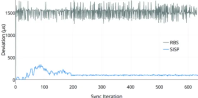
Figure 2 shows a graphical comparison of the RBS and SISP protocols for a two node network. The synchronization iteration (i.e., time samples) is on the X-axis and absolute clock error (i.e., the absolute value of the difference between the nodes’ synchronized clocks, called deviation) is on the Y-axis. This absolute clock error, or deviation, is measured from two motes. Each local clock sample is collected just prior to when synchronization occurs to obtain the likely maximum clock error for each time sample. Table I exhibits mean error, standard deviation, and 50%, 95%, and 99% percentile bounds for each protocol (e.g., for a 95% percentile bound, 95% of the absolute synchronization errors — that is, the absolute values of the synchronization errors — in a synchronization’s distribution are between 0 and the 95% percentile bound). Our results show that RBS is both significantly more imprecise (i.e., noisy) and inaccurate than SISP with equivalent config-urations on the same hardware. The large disturbances that occur during the start of the experiment for SISP are due to start-up costs in the network (i.e., the initial convergence to consensus). This period has not been included in the calculation of statistics in the “SISP (stable)” row of Table I. That is, the SISP row statistics in Table I take results from all synchronization intervals into account; while the SISP (stable) row statistics only make use of data from intervals after the start-up period (i.e., after 200 synchronization iterations).
While SISP has been shown to perform significantly better than RBS, can we design a protocol that does better than SISP? We want a time synchronization protocol that minimizes network traffic, is scalable, is resilient to dropped messages, is stable over significant periods of time, and is simple and lightweight in its implementation while also achieving a high degree of synchronization. In an n node network, a
TABLE I
RBSANDSISP SYNCHRONIZATIONERRORSTATISTICS
Protocol Mean Error (µs) Std Dev 50% Bound 95% Bound 99% Bound
RBS 1509 108 1528 1640 1744
SISP 119 78 96 192 421
SISP (stable) 96 5 96 104 104
Fig. 2. Comparison of RBS and SISP Synchronization Error
single SISP synchronization interval requires n transmissions and n ∗ (n − 1) receptions. If a new protocol was able to send and receive fewer messages per interval, the network’s synchronization frequency could be increased; furthermore, increasing the network’s synchronization frequency would lead to a higher level of synchronization, while still requiring fewer message transmissions and receptions per length of time than SISP.
IV. THESTICKINGHEARTBEATAPERTURE
RESYNCHRONIZATIONPROTOCOL
To improve upon existing protocols’ shortcomings, we have developed a master-slave, heartbeat-based protocol called Sticking Heartbeat Aperture Resynchronization Proto-col (SHARP). SHARP uses heartbeats emitted by a master node to synchronize slave nodes, without expressly knowing the master’s clock. The protocol is resilient to lost heartbeats and integrates seamlessly with networks that have scheduled protocols, such as TDMA. Additionally, SHARP does not require additional, non-standard radio hardware.
The Sticking Heartbeat Aperture Resynchronization Proto-col (SHARP) uses heartbeats (i.e., network messages contain-ing no data) for synchronization, and synchronization occurs even if heartbeats are dropped. Figure 3 provides an overview of SHARP, and illustrates how the protocol functions using a simple master-slave heartbeat propagation technique. A master node, which may or may not be synchronized with an external, absolute clock source, transmits a heartbeat to its slave nodes after every time period λ. This network’s synchronization interval length, λ, may be changed to fit a specific network’s time synchronization requirements. Figure 3 shows there are large, free spaces in the network where no synchronization takes place, allowing for the network to send other network communication or sleep the radios.
Fig. 3. SHARP Overview
A defining feature of SHARP is the existence of heartbeat apertures, i.e., time intervals where a heartbeat should occur. The length of the network’s heartbeat apertures is determined by a bound on a mote’s clock drift. When a heartbeat is received by a slave, the current aperture ends and the slave’s clock is adjusted to the master’s time, essentiallynλ, where n is the number of heartbeat apertures that have passed since the initial synchronization. The existence of heartbeat apertures enables TDMA to function with SHARP, i.e., the apertures can be easily included into the TDMA schedule.
Figure 4 demonstrates how the current interval’s clock skew, ∆n, is calculated for a given slave mote. Given a known λ, we calculate a node’s local clock shift change, δn, whenever a heartbeat is received:
δn= nλ − tlocaln+ ∆n−1,
wheretlocaln is the value of the local clock (i.e., the incorrect
clock that is provided by the hardware) at interval n. The current synchronization interval’s clock shift change, δn, is added to the previous interval’s clock shift,∆n−1, to find the current synchronization interval’s clock shift:∆n= ∆n−1+ δn.
A. Resilience
Heartbeat apertures provide resilience against lost heart-beats. We note theλ between heartbeats is constant, and that a mote’s clock does not drift significantly over a short period of time. Thus, a mote can estimate how many heartbeats,γn, it has missed since its last received heartbeat, i.e., a mote can count how many empty heartbeat apertures have passed. When the next heartbeat arrives, the mote’s clock can then snap to the
Fig. 4. Example Slave Clock Deviation
correct time, since the mote knows that γnλ time has passed since the last heartbeat. Specifically, SHARP may calculate a local clock shift change δn when a heartbeat is received, as before, by:
δn= nλ − tlocaln+ ∆n−1.
For heartbeat apertures where no heartbeat is received, the previous interval’sδn−1is used as the current interval’s clock shift change. Whenever a slave node misses a heartbeat, it adjusts the size of its next heartbeat aperture to be equal to the base aperture size multiplied by(γn+ 1). That is, SHARP assumes the slave’s clock’s skew increases as more heartbeats are missed, requiring larger heartbeat apertures to ensure that a future heartbeat is not missed. Once a heartbeat is received, the next heartbeat aperture can be restored to the base aperture size. SHARP is resilient to lost heartbeats up to the point where adjacent heartbeat apertures begin to overlap with each other.
B. Analytical Example
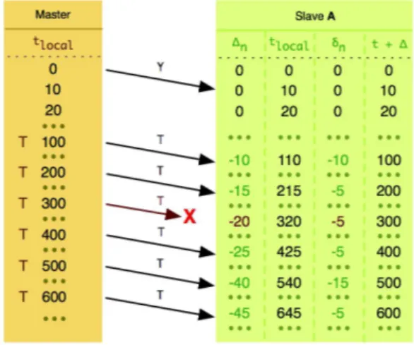
Figure 5 presents an example execution diagram for SHARP, detailing a master node and a slave node. LCLK represents the slave hardware’s reported clock value, tlocal, and SHIFT represents the slave’s local clock shift,∆. SHARP begins with an initial synchronization (i.e., a reliable, initial heartbeat that is acknowledged by all slaves), represented by Y in the figure. Following the initial synchronization, the master node transmits heartbeats periodically, every 100 units of time (i.e.,λ = 100). When the first heartbeat arrives, Slave A calculates that the heartbeat fits within the first heartbeat aperture; thus, Slave A adjusts its clock shift, ∆, so that ∆n+ tlocaln = n ∗ λ, where n is 1. The resultant δ1= −10,
meaning that the Slave A’s new ∆1 = ∆0+ (−10). This procedure continues for subsequent heartbeats. We note that the third heartbeat transmitted is not received by SlaveA; this missed heartbeat is handled gracefully by setting the current clock shift,δ3, to be the same as the previous clock shift,δ3−1. SlaveA then continues functioning normally.
C. SHARP Advantages
SHARP is computationally light, both spatially and tem-porally, requiring minimal data processing and state memory. Additionally, the protocol is energy efficient, requiring only
Fig. 5. SHARP Execution Example
0 5 10 15 20 25
CPU TX RX IDLE SLEEP SENSORS C u rr e n t (m A )
Fig. 6. Tmote Sky Current Draw [10]
one data reception per mote per synchronization interval. Thus, SHARP would work well in embedded networks requiring prompt data transmission and high data throughput.
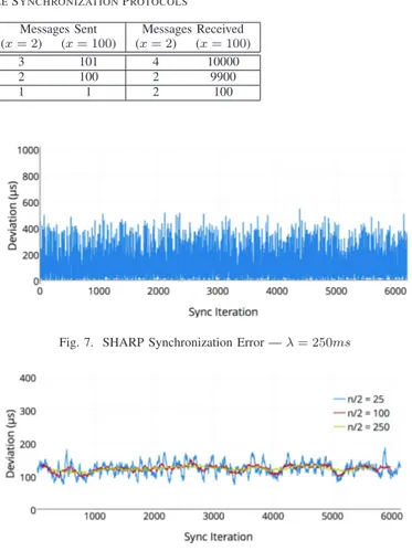
Table II provides a comparison of radio usage between SHARP and other time synchronization protocols. We detail transmission and reception counts symbolically for a network with an arbitrary number of motes, x, along with actual transmission and reception counts for networks with 2 and 100 motes. In this analysis, we assume a fully connected network. All figures are for a single synchronization interval. As shown, SHARP has significantly fewer messages sent and received than RBS and SISP. We note that high reception rates are sometimes more undesirable, energy-wise, than high transmission rates. For example; consider Figure 6, which details the current draw for different subsystems on a Tmote Sky wireless mote, a widely used wireless sensor network platform [10]. Lastly, note that Table II does not account for varying message sizes. That is, SHARP messages always have a zero-length payload, while SISP and RBS messages usually have a non-zero payload size.
Another major advantage of SHARP is that slave motes can be synchronized to an absolute time scale, unlike SISP which forms a relative time scale. For example, if the SHARP master is connected to an absolute time source, such as a rubidium frequency standard, thentlocalwould be the absolute time. This advantage exists in RBS as well, by providing the server node with an absolute time source. This feature is advantageous in applications where it is important to know
TABLE II
COMPARINGRADIOUSAGE OFTHREESYNCHRONIZATIONPROTOCOLS
Protocol Transmissions Receptions (x= 2)Messages Sent(x= 100) (xMessages Received= 2) (x= 100)
RBS 1 + x x+ x ∗ (x − 1) 3 101 4 10000
SISP x x ∗ (x − 1) 2 100 2 9900
SHARP 1 x 1 1 2 100
the actual, absolute time that an event occurred. V. SHARP RESULTS
We provide results and analyze the performance of SHARP in this section. We perform several test runs with different synchronization intervals. In our study, we report general statistics for each test run, along with absolute synchronization error plots, absolute synchronization error rolling mean plots with various window sizes, and calculated Root-Mean-Square Error (RMSE) values.
As expected, as the length of the synchronization interval, λ, is reduced, SHARP achieves progressively more accurate levels of synchronization. We find that SHARP exhibits a slightly higher synchronization error than SISP when compar-ing test runs with equal length synchronization intervals; how-ever, SHARP has a significantly lower number of messages transmitted and received. Thus, we can reduce the synchro-nization interval length,λ, in SHARP, allowing us to achieve a significantly lower network-normalized synchronization error than SISP, and still send fewer messages across the network. A. Analysis of Aggregate Statistics
Table III presents the mean error, standard deviation, and 50%, 95%, and 99% percentile bounds for SHARP, across different synchronization interval lengths. All provided statis-tics are from ∼ 7, 500 sample runs. As expected, the absolute clock error in the network generally reduces as the length of the synchronization interval, λ, is decreased.
Figure 7 presents how well SHARP synchronizes the clocks in a two-mote network for a synchronization interval of 250ms1. Time samples (taken just before each synchronization iteration, as before) are on the X-axis and absolute synchro-nization error (i.e., the absolute value of the difference between the two nodes’ synchronized clocks) is on the Y-axis. Each local clock sample is collected just prior to when synchro-nization actually occurs, in order to measure the maximum clock error.
B. Rolling Mean Analysis
Figure 7 illustrates how SHARP is extremely stable over time. This fact is especially clear in Figure 8, which presents rolling mean curves for the absolute synchronization errors in a network running SHARP at a synchronization interval of 250ms2. Rolling means were calculated for window sizes,
1Additional synchronization error graphs for intervals of 1000, 500, and
100 milliseconds are similar and available in [6].
2Additional rolling mean graphs for synchronization intervals of 1000, 500,
and 100 milliseconds are similar and available in [6].
Fig. 7. SHARP Synchronization Error — λ= 250ms
Fig. 8. SHARP Synchronization Error Rolling Mean — λ= 250ms
n, of 51, 201, and 501 samples, i.e., there are n/2 samples on each side of a center value that are averaged to produce a data point. The high level of stability offered by SHARP is important in the vast majority of wireless networks, where nodes are kept running for extended periods of time.
As window sizes are enlarged, e.g., yellow lines in the figures represent a larger window size than the blue lines in the figures, rolling mean data becomes progressively smoother. This result is expected since means are calculated from more data points when window sizes are larger.
C. RMSE Analysis
Root-Mean-Square Error (RMSE), sometimes referred to as Root-Mean-Square Deviation (RMSD), is an error metric that is commonly used. For a set of residuals,x1throughxk, RMSE is defined as follows:
RM SE = s Pk i=1x 2 i k
We compare the three time synchronization protocols — RBS, SISP, and SHARP — using RMSE in this section. RMSE does not need to be normalized for our comparisons
TABLE III
SHARP SYNCHRONIZATIONERRORSTATISTICS
Interval (ms) Mean Error (µs) Std Dev 50% Bound 90% Bound 95% Bound
1000 180 145 152 368 448
500 152 114 136 320 376
250 123 108 96 272 344
100 135 97 120 272 312
TABLE IV
COMPARISON OFSYNCHRONIZATIONPROTOCOLS VIARMSE Protocol Interval (ms) RMSE (µs) Mean Error (µs)
RBS 500 1512 1509 SISP 500 124 112 SISP 1000 189 179 SHARP 100 167 135 SHARP 250 162 123 SHARP 500 190 152 SHARP 1000 231 180
of the three protocols since the residuals all take place on the same time scale. RMSE is a good metric for evaluating time synchronization protocols as it penalizes error variability, i.e., peaks are taken into account more than troughs.
Table IV provides an RMSE comparison of SISP, RBS, and SHARP with different synchronization intervals. As an-ticipated, both SISP and SHARP exhibit significantly lower RMSE values than RBS. Additionally, when comparing runs of SISP and SHARP with equal synchronization interval lengths, SISP exhibits a slightly lower RMSE value. This result is due to the variability that is present in SHARP’s absolute synchronization error. We note, however, that SHARP is a successful protocol due to its low network usage, which allows for shorter synchronization intervals to be used. That is, SHARP can achieve a level of synchronization accuracy that is superior to that provided by SISP, while also transmitting and receiving fewer messages. For example, compare RMSE for SHARP, with λ = 500 (190µs), to RMSE for SISP, with λ = 1000 (189µs). These two RMSE values are similar, but SHARP only transmitted 2 messages per second while SISP transmitted 6 messages per second. This difference in transmission counts becomes more pronounced as network sizes are increased.
VI. CONCLUSION
As the number of wireless sensor network applications grows, the need for effective time synchronization has become clear. We present SHARP, a new protocol that improves upon the shortcomings of other protocols, while maintaining a high level of synchronization.
We initially evaluated RBS and SISP, two notable time synchronization protocols in the literature. RBS operates on the periodic transmission of “reference broadcasts” from a server node to trigger synchronization within a network. SISP operates in a completely distributed manner, where nodes achieve synchronization in a consensus based manner. Our
early results demonstrate that SISP is able to achieve a significantly lower average synchronization error than RBS on the same experimental setup. We note that RBS functions best on radios that support beacon messages (the Xbee radio modules do not), providing a possible explanation for the poor synchronization results we observed.
While SISP can achieve a reasonably high level of synchro-nization, it has several shortcomings, including the fact that many messages are transmitted per synchronization interval. As such, we developed the Sticking Heartbeat Aperture Resyn-chronization Protocol (SHARP), a simple, scalable, heartbeat-based protocol that meshes well with existing networks, espe-cially those that use TDMA. We then implemented SHARP on our GeoMote platform and extensively tested it. Experimenta-tion and analysis have deemed SHARP to be a great success; SHARP achieves synchronization accuracy that is comparable or better than that provided by SISP, while transmitting and receiving vastly fewer messages, resulting in lower network and energy usage.
Our hope is that SHARP can be augmented over time to become a de facto protocol for time synchronization in TDMA-based networks and wireless sensor networks. SHARP provides numerous advantages that, coupled with its excellent synchronization performance, make it a great choice for wire-less applications.
We plan to improve SHARPs synchronization accuracy in future works by learning relative clock drifts between slave nodes and the master node and compensating for them over time. An important issue to be tackled as well is to determine an energy-efficient aperture size [11] and beaming period λ [12]. Relevant recent works tackle similar issues that could be leveraged to augment the network lifetime together with an improved synchronization precision.
ACKNOWLEDGMENT
The authors are thankful for the support of the National Science Foundation under Grant No. OISE-1243539. Any opinions, findings, conclusions, or recommendations expressed in this material are those of the author(s) and do not necessarily reflect the views of the National Science Foundation.
REFERENCES
[1] J. Elson, L. Girod, and D. Estrin, “Fine-grained network time synchro-nization using reference broadcasts,” Proceedings of OSDI, 2002. [2] A. V. D. Bossche, T. Val, and R. Dalce, “SISP: a lightweight
synchro-nization protocol for wireless sensor networks,” Proceedings of ETFA, pp. 1 – 4, 2011.
[3] P. Juang, H. Oki, Y. Wang, M. Martonosi, L.-S. Peh, and D. Rubenstein, “Energy-efficient computing for wildlife tracking: Design tradeoffs and early experiences with zebranet,” Proceedings of ASPLOS-X, 2002. [4] S. Kim, S. Pakzad, D. Culler, J. Demmel, G. Fenves, S. Glaser, and
M. Turon, “Health monitoring of civil infrastructures using wireless sensor networks,” Proceedings of IPSN, 2007.
[5] F. Sivrikaya and B. Yener, “Time synchronization in sensor networks: A survey,” IEEE Network, vol. 18, pp. 45–50, 2004.
[6] S. Gonzalez, “Improving time synchronization protocols in wireless sensor networks,” Master’s thesis, Colorado School of Mines, 2015. [7] D. L. Mills, “Internet time synchronization: The network time protocol,”
IEEE Transactions on Communications, vol. 39, no. 10, pp. 1482–1493, 1991.
[8] S. Ganeriwal, R. Kumar, and M. B. Srivastava, “Timing-sync protocol for sensor networks,” Proceedings of SenSys, pp. 138–149, 2003. [9] T. Camp, M. Rubin, and S. Gonzalez, “Challenges in developing
intelligent geosystems (and the pros/cons of interdisciplinary research),” Proceedings of ICNC, 2015.
[10] W. Heinzelman. Wireless sensor networks: Past, present, and future. Accessed on October 14, 2015. [Online]. Available: http://www.cs.rit.edu/ spr/CLQABS/wendi.pdf
[11] Y. Chen, F. Qin, and W. Yi, “Guard beacon: An energy-efficient beacon strategy for time synchronization in wireless sensor networks,” IEEE Communications Letters, vol. 18, no. 6, pp. 987–990, June 2014. [12] J. P. B. Nadas, R. D. Souza, M. E. Pellenz, G. Brante, and S. M. Braga,
“Energy efficient beacon based synchronization for alarm driven wireless sensor networks,” IEEE Signal Processing Letters, vol. 23, no. 3, pp. 336–340, March 2016.