A Low-Cost Automated Test Column to Estimate Soil Hydraulic Characteristics in Unsaturated Porous Media.

(1)

Research Article

A Low-Cost Automated Test Column to Estimate Soil Hydraulic

Characteristics in Unsaturated Porous Media

J. Salas-García,

1

J. Garfias,

1

R. Martel,

2

and L. Bibiano-Cruz

1

1_{Faculty of Engineering (CIRA), Autonomous University of the State of Mexico, Toluca, MEX, Mexico}

2_{Institut National de la Recherche Scientifique (INRS-ETE), Qu´ebec, QC, Canada G1K 9A9}

Correspondence should be addressed to J. Garfias; jgarfiass@gmail.com

Received 5 July 2016; Revised 18 December 2016; Accepted 4 January 2017; Published 24 January 2017 Academic Editor: Cinzia Federico

Copyright © 2017 J. Salas-Garc´ıa et al. This is an open access article distributed under the Creative Commons Attribution License, which permits unrestricted use, distribution, and reproduction in any medium, provided the original work is properly cited. The estimation of soil hydraulic properties in the vadose zone has some issues, such as accuracy, acquisition time, and cost. In this study, an inexpensive automated test column (ATC) was developed to characterize water flow in a homogeneous unsaturated porous medium by the simultaneous estimation of three hydraulic state variables: water content, matric potential, and water flow rates. The ATC includes five electrical resistance probes, two minitensiometers, and a drop counter, which were tested with infiltration tests using the Hydrus-1D model. The results show that calibrations of electrical resistance probes reasonably match with similar studies, and the maximum error of calibration of the tensiometers was 4.6% with respect to the full range. Data measured by the drop counter installed in the ATC exhibited a high consistency with the electrical resistance probes, which provides an independent verification of the model and indicates an evaluation of the water mass balance. The study results show good performance of the model against the infiltration tests, which suggests a robustness of the methodology developed in this study. An extension to the applicability of this system could be successfully used in low-budget projects in large-scale field experiments, which may be correlated with resistivity changes.

1. Introduction

The unsaturated soil hydraulic functions are important parameters in many soil, hydrological, ecological, and agri-cultural studies (e.g., [1, 2]). Thus, the estimation of the unsat-urated flow should be precisely analyzed; their evaluation has important implications in transient process of infiltration due to the high nonlinearity of soil water characteristics. It is also crucial in evaluating the dynamics of chemical pollutants in soil and in assessing the risks of groundwater pollution. However, the available methods to obtain soil hydraulic parameters are often difficult to implement in practice, as well as being time-consuming [3]. According to Mertens et al. [4], this task is not trivial, since soil moisture exhibits high variability in time and space. These issues have prompted the development of analytical and numerical methods to calculate parameters that are difficult to measure in the field [5, 6].

However, the implementation of modeling tools is ham-pered by the lack of field data, needed to assess the capability

of models and approaches. Consequently, the estimation of the hydraulic properties in porous media is an essential issue. For many years, monitoring methods have lagged behind numerical analyses of water flow, solute transport, and heat transfer into and through the vadose zone. Nevertheless, recent advances in electronic components, renewed interest in development of monitoring methods, and the infusion of new electromagnetic sensors into vadose zone hydrology have begun to address this imbalance [7].

In order to solve time-consuming measurements issues, automated devices are increasingly being used to evaluate soil hydraulic properties to examine the nature of water flow dynamics. Thus, the most common instruments are automated infiltrometers and permeameters [8, 9]. However, more information is often required compared to only the measurements made at the soil surface. Depending on the objective of the study, it is frequently necessary to estimate vadose zone parameters from laboratory and in situ tests. These include methods for full-scale infiltration evaluation of various intensities simulated rainfalls and durations over Volume 2017, Article ID 6942736, 13 pages

(2)

a selected area [10] to analyze flow behavior in small soil samples (cm3 in size) such as those needed for X-rays diffraction [11].

Hydrological models able to simulate soil moisture con-tent profiles using Richards [12] equation require two soil hydraulic functions: the soil water retention curve and the hydraulic conductivity curve. The parameters of these func-tions can be estimated by analyzing soil cores in the labora-tory or from in situ measurements. In a modeling context, soil moisture content and matric potential measurements can be used to estimate effective soil hydraulic parameters using the inverse method introduced by Zachmann et al. [13]. Although the inverse method can be an effective alternative, it occasionally produces nonunique solutions. Parker et al. [14] showed that the inverse method for a one-step outflow experiment did not produce a unique estimate when there were three unknown parameters and only outflow volume was measured. Russo et al. [15] and ˇSim˘unek and van Genuchten [16] obtained similar results, which suggests that uniqueness of the one-step outflow experiment could be improved by incorporating additional variables (e.g., water contents and/or pressure heads) to yield a unique solution. Hence, the effectiveness with which these modeling tools in environmental management can be adopted relies heavily on the quality with which unsaturated flow parameters can be identified.

Considering the complexity of processes occurring in the unsaturated zone, and the need of automatized data acquisition, the main goal of this paper is to present an automated test column (ATC) to perform laboratory tests to determine a set of hydraulic properties from homoge-neous soil samples and to demonstrate their suitability in a one-dimensional model (Hydrus-1D) to simulate transient infiltration associated with unsaturated soil water flow. The research approach includes a combined use of direct and indirect methods to estimate soil hydrodynamics parameters in unsaturated soils aiming to(1) evaluate the information content of different types of measurements (water content, matric potential, and soil water fluxes) collected from an automated system under different boundary conditions and herein verify the performance of the sensors installed, (2) identify the model parameters from the available data con-taining the most rich information content, and(3) investigate the simulated transient water contents and water fluxes against the measured data to provide an independent veri-fication of the model. The results not only demonstrate the utility of various investigational approaches to evaluate the flow system dynamics in unsaturated soils but also provide an insight on the performance, reliability, and usefulness of these probes.

2. Materials and Methods

The research approach involved three main components. First, the experimental setup of the column test and their operational principles associated with calibration and mea-surement of hydraulic state variables are presented. Second,

a description of the infiltration tests and boundary condi-tions, that are used as input in a one-dimensional modeling approach (Hydrus-1D), are shown to conduct a quantitative assessment of soil hydraulic functions and water fluxes in the column experiment. Finally, simulated and measured output values were compared and differences were quantified with statistical performance criteria to evaluate the ATC system.

2.1. Experimental Setup. The laboratory experimental setup

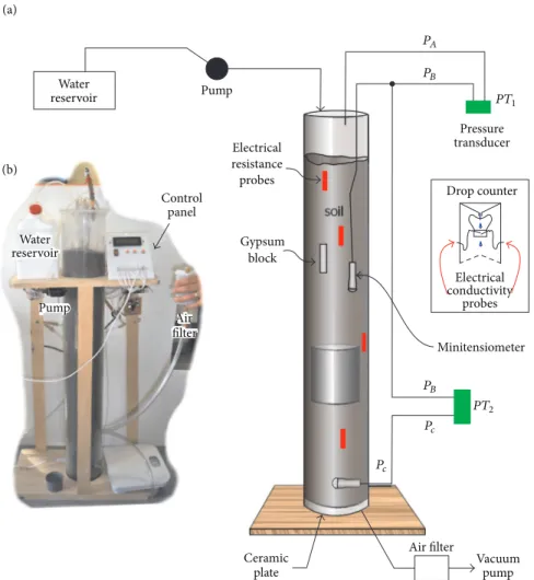
allowed performing infiltration experiments in a column with controlled boundary conditions while monitoring dif-ferent hydraulic state variables. Column studies were con-ducted using an acrylic column with an inner diameter of 12.7 cm and a length of 1.15 m filled with a homogeneous sand. Schematic details of the column test apparatus and experimental column setup are illustrated in Figure 1, includ-ing external components used for drainage experiments. In this schema, at the top of the column, a pump provides the incoming water from a 5 L water storage reservoir. For controlled drainage, the column was equipped with a porous ceramic suction plate at the bottom to apply a defined lower boundary pressure head condition via different setting of the connected vacuum pump (0 to−50 kPa). The column design (Figure 1) was similar to the one used by Ritter et al. [20] and Scholl et al. [21].

In this context, five devices were developed based on electrical resistance that continuously measure changes in moisture content. Each of them consists of two unshielded copper wires, 3 mm in diameter and 8 cm high, mounted on both sides of a 5 mm thick acrylic separator. Four of them are in direct contact with the porous media to provide a quick response, while the fifth resistance probe is embedded into a gypsum block, which reduces the electrical resistance differences between measures with different salinity degrees, thus providing more stability to measure moisture content in the soil column [22]. As a result of this system, the electrical resistance measured by the probes is converted into volumetric water content of the soil by a calibration curve.

All electrical resistivity probes are connected to the same electronic resources by means of an analog multiplexer. The electrical resistance, 𝑅, is measured in terms of an output frequency function,𝑓, from a NE555 oscillator circuit in a stable configuration according to the following equation [23]:

𝑓 =_{𝐶 (𝑅} 1

𝑎+ 2𝑅) ln 2, (1)

where 𝑅_𝑎 is the resistance in ohms (Ω) and 𝐶 is the capacitance in farads (F). Both𝐶 and 𝑅_𝑎are fixed values of the oscillator circuit, whereas𝑅 varies according to water content in the column test. The analog multiplexer selects sequentially the signal from each monitoring probe and forwards it to the oscillator circuit. The main advantages of this configuration are as follows: (1) since alternate current is applied to the probes, it does not generate gasses and apparent resistance changes [22],(2) 𝐶 and 𝑅_𝑎values are the same for all probes, and(3) it minimizes the amount of electronic components included in the devices.

Additionally, the system was instrumented with two minitensiometers installed in the soil column at two

(3)

Electrical resistance probes Control panel Water

reservoir Gypsum_block

Air filter Water reservoir Pump (a) (b) Ceramic plate Air filter Vacuum pump Pressure transducer Drop counter Electrical conductivity probes Minitensiometer PB PA PB PT2 PT1 Pc Pc Pump

Figure 1: (a) Schematic representation of the experimental design of the automated test column (ATC) and (b) photograph showing the external components used for drainage experiments.

observation depths to measure the matric potential (Fig-ure 1), each connected to a differential press(Fig-ure transducer MPXV5050DP [24]. In order to equilibrate with the moisture in the soil column, the tensiometers were partially filled with water before inserting them into the soil column used for drainage experiments. The difference of pressure between𝑃_𝐴 and𝑃_𝐵is measured by𝑇₁, whereas the difference between𝑃_𝐵 and𝑃_𝐶is measured by𝑇₂. The pressure range of both sensors goes from 0 to−50 kPa. The output voltage from transducers 𝑇1and𝑇2is coupled to an analog-to-digital converter to be processed by a PIC18F4550 microcontroller [25].

A collector, equipped with a drop counter, was used to measure the volume of water that flows down through the column during each experiment by either gravity or external pressure (Figure 1). The drop counter consists of a funnel with a hydrophilic synthetic material attached to its small opening. It leads the captured water towards a signal-conditioning circuit coupled to the microprocessor. Thus, when a drop of water falls down, it flows between two conductivity probes and closes the circuit. The microprocessor counts the amount of water drops detected in a period of time, then this is converted into milliliters minute−1 (mL min−1) units. In

addition, it is possible to transfer the measured data to a computer via a USB (Universal Serial Bus) port.

2.2. Calibration and Measurement of Hydraulic State Vari-ables. In order to calibrate the resistance probe inside the

gypsum block, the water content from several samples was determined by a gravimetric method, which is widely used to calibrate indirect water content measurements [26, 27]. In this approach, the sample is weighed before and after being dried; the difference between the two masses constitutes the water content. Thus, the sample was dried in an oven at 110∘C until its weight does not change. The time to reach this state depends on the volume sampled, soil characteristics, and water content [26, 28].

The calibration of tensiometers was obtained by means of four vacuum pressure (suction) values over a range of−50 to 0 kPa generated by a vacuum pump. As a second calibration method, falling-head tests using a water-filled column were performed with each tensiometer with a pressure span from −20 to 0 kPa. The falling-head tests were carried out at rates greater than the wetting front velocity observed in the soil column experiment. Similar calibration processes have been carried out by Bathurst et al. [29], who investigated the

(4)

transient unsaturated-saturated hydraulic response of sand-geotextile layers under 1D constant-head surface infiltration conditions.

The calibration of the collector, including the drop counter to measure the flux of water, was initially tested out of the column, where laboratory multipoint calibrations were conducted by the addition of five known volumes of water at the top of the collector and counting the drops for each case. The hydrophilic material was dry at first, and it was required to overpass a threshold until the material became saturated and starts dripping. The corresponding volume was measured from the moment when the first drop was detected by the sensor. Once the calibration of devices has been achieved, the next step was to measure the hydraulic state variables in the soil column experiment. Therefore, throughout each infiltration experiment, matric potential, soil water content, and water fluxes were recorded at 10 min increments and then averaged at 1 h intervals.

2.3. Infiltration Tests and Boundary Conditions. In the present

study, three infiltration tests were developed to investigate the effects of different boundary conditions and verify the performance of the sensors installed in the automated col-umn test (ATC). During these tests, data from electrical resistance probes, a gypsum block, and a drop counter were recorded using different experimental setups. Thus, a first experiment was performed to obtain information about the soil hydraulic functions in the column test. In this context, the lower boundary during the drainage experiment was set to a constant pressure head of−50 kPa (Dirichlet condition). At the upper boundary, an infiltration flux of 5 mm h−1 was applied until a steady outflow rate was achieved as initial condition. Thereafter, infiltration was stopped and matrix potential and water content were monitored during the redistribution phase. Soil surface was covered by parafilm to avoid evaporation (i.e., no flux upper boundary condition), while, at the lower boundary, drainage continued under a constant pressure head of−50 kPa. The transient profiles of water content and matrix potential during the redistribution phase entered the evaluation procedure for hydraulic prop-erty estimation.

A second infiltration experiment was performed to obtain information about the advancement of the wetting front in the column test. In that case, the top of the column was designed to provide a constant head of water to simulate surface recharge of a soil mass due to infiltration of ponded water. The depth of ponded water at the top of the column was maintained at 3 mm during 75 min using the reservoir placed on the top of the column (4 L). Following the end of the 75 min infiltration flux, the column was allowed to drain for 8 h to measure water content and water flow profiles. At the bottom of the column, the value of the pressure head is constant and equivalent to atmospheric pressure. This type of boundary condition at the column outlet automatically describes free outflow from the soil column.

A third drainage experiment was performed subsequently to obtain a validation data set. Thus, in the third test, 8.6 L of water was pumped from the reservoir located on the top of the column, respectively. The infiltration rate

was set at 1 cm high at the upper boundary to provide a constant head due to infiltration of ponded water and drained under the same conditions as described previously, whereas a suction generated by a vacuum pump was applied at the bottom boundary (−50 kPa). In this scenario, the transient profiles of water content and water flux obtained during the redistribution phase where compared with simulated values (Hydrus-1D) to assess the performance of the sensors.

2.4. Unsaturated Water Flow Modeling. The simulations of

the one-dimensional (1D) vertical water flow model were carried out using the Hydrus-1D model [30]. The latter is widely used to simulate water flow and solute transport through the vadose zone (e.g., [31, 32]). The Hydrus-1D pro-gram numerically solves the Richards equation for saturated and unsaturated water flow and the convection-dispersion equations for heat and solute transport. The governing one-dimensional water flow equation for a partially saturated porous medium is described using the modified form of the Richards equation, under the assumptions that the air phase plays an insignificant role in the liquid flow process and that water flow due to thermal gradients can be neglected:

𝜕𝜃 (ℎ) 𝜕𝑡 = 𝜕 𝜕𝑧[𝐾 (ℎ) ( 𝜕ℎ 𝜕𝑧+ 1)] , (2)

whereℎ is the matrix potential in cm, 𝐾(ℎ) is the unsaturated hydraulic conductivity function in cm⋅day−1_,_{𝑧 is the depth} in cm (positive in the opposite direction to gravity),𝜃 is the volumetric water content in cm3⋅cm−3, and𝑡 is the time in days.

To solve (2), the retention function,𝜃(ℎ), the hydraulic conductivity function, 𝐾(ℎ), and the initial and boundary conditions need to be defined. According to van Genuchten [17], they are given as follows:

𝜃 (ℎ) = 𝜃𝑟+_{[1 + (𝛼ℎ)}𝜃𝑠− 𝜃𝑟𝑛_]𝑚 ℎ < 0, (3)

𝜃 (ℎ) = 𝜃𝑠 ℎ ≥ 0, (4)

𝐾 (𝜃) = 𝐾𝑠𝑆𝑒𝑙(1 − (1 − 𝑆𝑒1/𝑚)𝑚) 2

, (5)

where𝐾_𝑠is the saturated hydraulic conductivity in cm⋅day−1, 𝑆_𝑒 = (𝜃 − 𝜃_𝑟)/(𝜃_𝑠− 𝜃_𝑟) is the effective saturation (nondimen-sional), and𝑙 is a factor that accounts for the pore connectivity or pore tortuosity (nondimensional);𝜃_𝑠is the saturated water content in cm3⋅cm−3; 𝜃_𝑟 is the residual water content in cm3⋅cm−3;𝑚, 𝛼, and 𝑛 are empirical shape parameters, where 𝑚 = 1 − 1/𝑛. A high value of 𝑙 corresponds to a low pore connectivity or a high pore tortuosity.

2.5. Estimation of the Parameters of the Hydraulic Functions.

Direct and indirect methods are available to estimate soil hydraulic properties, which are prerequisites to solve water movement equations. Direct methods are usually time-consuming and require measuring devices and a skilled operator compared to indirect methods. Indirect methods, for example, pedotransfer functions (PTFs), which estimate

(5)

parameters based on easily obtained soil texture data, have lately been widely used. However, the reliability of these parameters should be scrutinized, because PTFs are based on general data sets, and verification with true field data is often lacking. During this research, we investigate how well a combination of direct and indirect methods estimates soil hydraulic parameters that are used as input in a one-dimensional (Hydrus-1D) vertical water flow model to simu-late water balance variables, such as soil water content. Thus, these simulated data are compared to experimental data using controlled experiments at the column scale assuming one-dimensional water flow.

In this regard, ROSETTA, developed by United State Salinity Laboratory (USSL), a neural network model, was executed to obtain initial values of soil hydraulic parameters [33]. ROSETTA allows obtaining continuous and class PTFs. In this study, continuous PTFs are obtained using average of sand, silt, and clay percentages along with bulk density. The bulk density,𝜌_𝑏, from laboratory measurements has a value of 1.92 g⋅cm−2_{. Furthermore, an estimate of saturated hydraulic} conductivity was obtained from falling-head permeameter tests performed on repacked samples [34]. The ROSETTA software was used in several studies (e.g., [35, 36]).

In the present study, the state variables considered are soil water content (𝜃), matric pressure head (ℎ), and vertical flow rates through the soil column (𝑞), which were measured in the laboratory using the automated devices installed in the column. To convert retention data to the retention function parameter using the user-friendly software named RETC (RETention Curve), a computer program developed by USSL was executed. During this research, two approaches were used to determine a set of hydraulic parameters from the infiltration tests. In the first approach, the initial estimates of flow parameters (soil hydraulic parameters) were taken from the ROSETTA program and used as prior information in the estimation of optimized soil parameters for modeling the soil water content in the column experiment. According to Mertens et al. [4], the effective parameter estimates are more realistic when the prior information is incorporated. As an alternative, in the second approach, the initial estimates of the soil hydraulic parameters were taken based on a literature review of previous studies as a first guess for the RETC program [20, 21, 37].

RETC uses a nonlinear least-squares optimization approach to estimate the unknown model parameters from observed hydraulic state variables and/or conductivity data. The model allows for the optimization of any one, several, or all hydraulic function parameters, including 𝜃_𝑟, 𝜃_𝑠, 𝛼, 𝑛, 𝑚, 𝑙 and 𝐾_𝑠. For the present study, RETC is executed to obtain retention parameters, namely, 𝜃_𝑠, 𝜃_𝑟, 𝛼 and 𝑛 only from observed hydraulic state data. Note that the number of parameters to be estimated depends on the availability and suitability of the data. For example, in most cases,𝜃_𝑠 is available from the experiment, and, therefore, it is not optimized. Likewise, the 𝑙 parameter was not measured in laboratory and set to its typical value of 0.5 [38], and the saturated hydraulic conductivity (𝐾_𝑠) was measured using the laboratory constant-head technique. As mentioned above, the parameter sets from these estimation methods were used

in Hydrus-1D, a one-dimensional variable saturation soil water model, to simulate the advancement of the wetting front in the third column test using the same boundary conditions. The calibration of the model was carried out by trial-and-error iterative procedure; an extensive parameters optimization analysis was not performed because it was not the focus of this study.

2.6. Model Performance Analysis. The model performance

analysis was evaluated by five statistical analysis criteria: the maximum error (ME); root mean square error (RMSE); coefficient of determination (𝑅2_{); modeling efficiency (EF);} and coefficient of residual mass (CRM). Their mathematical expressions are widely defined in hydrological literature (e.g., [39]). The lower limit for ME, RMSE, and 𝑅2 is zero and the maximum value for EF and 𝑅2 is one. Both EF and CRM can be negative. A high value of ME represents a poor model performance, while a large RMSE value shows how much the simulations overestimate or underestimate the measurements. A negative EF value indicates that the averaged measured values give a better estimate than the sim-ulated values. The CRM is a measure of the tendency of the model to overestimate or underestimate the measurements. A negative CRM shows a tendency to overestimate. If all simulated and measured values are the same, these statistics would be ME = 0, RMSE = 0,𝑅2= 1, EF = 1, and CRM = 0.

3. Results and Discussion

3.1. Calibration of Sensors Installed in the Soil Column.

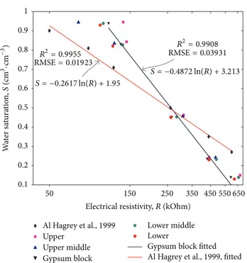
Figure 2 shows the water saturation, defined as the water content divided by porosity, versus electrical resistivity for the gypsum block sensor installed in the ATC. As shown in this figure, the calibration obtained only takes into account the gypsum block sensor, due to the fact that this device provides more stability to measure moisture content in the soil column. It includes also the resistivity values of a similar calibration in a sandy soil obtained by Al Hagrey et al. [10]. As illustrated in Figure 2, the relationship between resistance to water content in both probes has the same behavior; that is, the greater the soil water saturation, the smaller the resulting resistance. Nevertheless, the full range is different due to the fact that electrical resistivity is a geometry-dependent variable, which varies according to materials and dimensions of the probes. From this study, the slope of the plot is slightly higher than that reported by Al Hagrey et al. [10] due to different porosities (𝜙 = 0.37 in [10] and 𝜙 = 0.275 in this study) and the geometry of the sensors. Hence, taking into consideration the results, it is evident that the calibrated values provide reasonable estimates to describe the laboratory electrical resistivity data.

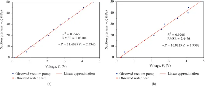
In order to assess the response of the tensiometers, Figure 3 displays the relationship between the suction pres-sure,𝑃_𝑠, versus the output voltage,𝑉_𝑡, for both tensiometers (𝑃𝑇₁and𝑃𝑇₂) obtained by two calibration methods. In this context, in the calibration using data obtained with a vacuum pump (indicated by squares), the maximum difference in respect to the linear approximation for𝑃𝑇₁occurred at 5 kPa.

(6)

W at er s at ura tio n ,S (cm 3 ·cm − 3 ) 50 150 250 350 450 550 650

Electrical resistivity, R (kOhm)

0.1 0.2 0.3 0.4 0.5 0.6 0.7 0.8 0.9 1 Al Hagrey et al., 1999 Upper Upper middle Gypsum block Lower middle Lower

Gypsum block fitted

Al Hagrey et al., 1999, fitted

R2= 0.9955 R2= 0.9908 RMSE = 0.01923 RMSE = 0.03931 S = −0.2617 ln(R) + 1.95 S = −0.4872 ln(R) + 3.213

Figure 2: Calibration of the water saturation versus electrical resistivity (gypsum block) determined through the sensors used in this study compared to the results of a similar calibration obtained by Al Hagrey et al. [10].

This difference of 148 mV represents an error of 3.2% in respect to the full range. Moreover, for the sensor𝑃𝑇₂, the maximum difference was detected at 40 kPa, which repre-sents an error of 4.6%. As expected, for the second calibration method, similar results were obtained using a negative water head pressure (indicated by circles). In this scenario, the maximum error in respect to the full span was 2.7% and 2.8% for𝑃𝑇₁and𝑃𝑇₂, respectively. Taking into consideration the above results, the voltage response shows a high linear correlation with a value of 𝑅2 = 0.9965 for 𝑃𝑇₁ and 𝑅2 = 0.9905 for 𝑃𝑇₂. This is due mainly to the design of the transducers themselves, based on a variety of techniques and standards in both laboratory and field studies, which includes a linearization stage and a temperature compensation circuit [40].

On the other hand, results of the drop counter calibration in terms of the volume of water applied at the upper boundary versus the number of water drops detected by the device are observed in Figure 4, which shows that the calibrated values suggest a general agreement between simulated and observed data. In this schema, the line represents the linear approxi-mation with coefficient𝑅2 = 0.9974 and a RMSE = 0.0018. The measured values had an average of 29.88 microliters (𝜇L) per drop and a standard deviation of 0.236𝜇L. Furthermore, the travel time of the water drops between the drop counter probes was approximately 50.4 ms, which means that the drop counter can measure up to 1190 drops per minute. Therefore, the maximum rate that the drop counter may measure is 35.57 mL⋅min, corresponding to an infiltration rate of 2.19 mm min−1, which exceeds widely the amount of

effective rainfall that can infiltrate in the vadose zone. In that context, the soil does not allow such high infiltration rate, due to runoff that occurs when the surface becomes saturated, in which the effective rainfall intensity exceeds the infiltration capacity of the soil.

3.2. Estimation of the Water Retention Curve. As illustrated

in this study, the first approach, derived from a combined approach based on the van Genuchten model (ROSETTA) to obtain initial values of soil hydraulic parameters and the RECT model, gives similar results for the estimation of optimized soil parameters. The main difference between both is the number of iterations: 86 iterations when using the combined approach with ROSETTA against 106 iterations when using only the RETC program. Hence, Figure 5(a) presents the water retention data obtained from laboratory experiments, as well as the retention function (RF) based only on the second approach (RECT model). In this representa-tion, the optimized retention function (RF) was compared to other water retention curves obtained by Carsel and Parrish [18] based on 12 major soil textural groups. It can be seen that the resulting fitted curve is a reasonable agreement between the simulated and measured points, except for measurements performed in low water contents, which could be associated with sensitivity of suction observed at high pressure values.

According to the USDA soil texture triangle, the soil particle distribution used in this study to obtain soil hydraulic parameters is classified as sand soil. For this reason, in the present study, the comparison between soil hydraulic functions was developed with similar soil textures, taking into account sand, sandy loam, and loamy sand data, as can be seen from Figure 5(a). As indicated in this graph, a comparison between the soil hydraulic function of this study (sand) and the retention function for the same soil data (sand) differs significantly for low water content and near saturation where, for the same matric, potential the water content values present significant differences. Such results do not correspond to those obtained by Paige and Hillel [41] who found close agreement for the moisture retention relation-ships determined by the instantaneous profile method and the soil cores. According to Islam et al. [37], this may be due to differences in input components into the methods to estimate the hydrodynamics parameters. On the other hand, for loamy sand and sandy loam, both approaches lead to relatively close results, as they even overlap in some instances, especially for the RF obtained using loamy sand.

As explained by Islam et al. [37], clay soils usually have higher𝜃_𝑠and𝜃_𝑟 but lower𝛼 (i.e., higher bubbling pressure) and𝑛 (i.e., gradual decrease of water content with an increase of matric head) than sandy soils due to pore size distribution differences. In this research, however, mixed and reverse patterns of these parameters are observed (Table 1), which is contrary to observed soil particle distribution data. The higher 𝜃_𝑠 and 𝑛 for sand soil data taken from Carsel and Parrish [18] make the RF distinct from others at low and higher water contents. A relatively low value of 𝑛= 1.89 is obtained for sandy loam (Table 1), which results in a steeper retention curve in Figure 5(a). Similarities between the retention functions are more obvious for sand of this

(7)

0 1 2 3 4 5 Voltage, Vt(V) 0 10 20 30 40 50 Su ct io n p ressur e, −P s (kP a)

Observed vacuum pump

Observed water head

Linear approximation R2= 0.9965 RMSE = 0.08181 −P = 11.4025 Vt− 2.3945 (a) 0 10 20 30 40 50 Su ct io n p ressur e, −P s (kP a) 1 2 3 4 5 0 Voltage, Vt(V)

Observed vacuum pump

Observed water head

Linear approximation

R2= 0.9905

RMSE = 2.4476

−P = 10.8225 Vt+ 1.9588

(b)

Figure 3: Calibration results of tensiometers: (a)𝑇₁and (b)𝑇₂expressed as suction pressure,𝑃_𝑠, versus voltage from the transducers,𝑉_𝑡, using a vacuum pump (circles) and a negative water head pressure (squares) applied at the bottom boundary.

Table 1: Soil hydraulic parameters for different soils used to estimate the soil hydraulic functions according to the formulation of van Genuchten [17] (Figure 5). Soil 𝜃_𝑟(cm3cm−3) 𝜃_𝑠(cm3cm−3) 𝛼 (cm−1) 𝑛 (—) 𝑚 (—) 𝑙 (—) 𝐾_𝑠(cm⋅h−1) Sand∗ 0.045 0.430 0.145 2.680 0.627 0.5 29.70 Sandy loam∗ 0.065 0.410 0.075 1.890 0.471 0.5 4.42 Loamy sand∗ 0.057 0.410 0.124 2.280 0.561 0.5 14.59 ATC sand 0.055 0.420 0.130 1.900 0.474 0.5 21.00

∗_{Values extracted from Carsel and Parrish [18].}

0 20 40 60 80 100 V o lu me , V o l (mL) Rela ti ve er ro r (%) −0.30 −0.25 −0.20 −0.15 −0.10 −0.05 0.00 0.05 1 2 0 0.2 0.4 0.6 0.8 1.2 1.4 1.6 1.8 Number of drops ×103, Nd(—) R2= 0.9974 RMSE = 0.0018 Vol = 0.04987 Nd

Observed (left axis)

Linear approximation (left axis) Relative error (right axis)

Figure 4: Calibration results of the drop counter expressed as vol-ume of water (left axis) added at the upper boundary versus number of drops,𝑁_𝑑, detected by the sensor. The linear approximation (left axis) and the relative error (right axis) are also included.

study and loamy sand. However, no consistency in soil hydraulic functions for the same soil texture is apparent.

Moreover, Figure 5(b) shows the unsaturated hydraulic conductivity data obtained from functions predicted by (5)

using the retention properties and the saturated hydraulic conductivity values measured in the laboratory (Table 1). In this graph, the measured unsaturated hydraulic conductivity data is not showed because it was not determined experi-mentally. It is evident from Figure 5(b) that the shape of the profiles is reasonably well fitted according to the model of van Genuchten [17], showing a rapid decrease of the unsaturated hydraulic conductivity near saturation. In this schema, there is a comparison that shows that the unsaturated hydraulic conductivity determined using sand data from Carsel and Parrish [18] is systematically higher than those predicted from the laboratory at the column scale for low matric potential values. Similarly, a comparison of the results for the same curve is less satisfactory in the high matric potential range. According to Mermoud and Xu [42], this could be associated with differences in volume scale of measurement involved in the two approaches and with a possible influence of macropores on the transmission characteristics of the soil. On the other hand, loamy sand data provide hydraulic functions relatively close to the predicted data of this study, except for high matric potential values where the curves show more differences than similarities.

In summary, considering both, retention and conductiv-ity functions, one can consider that, in the context of the experimental column scale, the approach based on experi-mental data of this study to estimate soil hydraulic parameters

(8)

0 0.05 0.1 0.15 0.2 0.25 0.3 0.35 0.4 0.45 Water content, 𝜃 (cm3/cm3) 10−2 10−1 100 101 102 103 104 M atr ic p o te n tial , Sand Loamy sand Sandy loam

ATC sand, simulated ATC sand, observed

−𝜓 (cm) (a) Sand Loamy sand Sandy loam ATC sand, simulated

10−6 10−5 10−4 10−3 10−2 10−1 100 101 102 10−3 10−2 10−1 100 101 102 103 H ydra ulic co nd uc ti vi ty ,K (cm/h) Matric potential,−𝜓 (cm) (b)

Figure 5: (a) Plot of water retention function for different unsaturated porous media using the soil parameters presented in Table 1, according to the formulation of van Genuchten [17] and (b) unsaturated hydraulic conductivity as a function of matric potential by using soil hydraulic parameters included in Table 1 and (5).

W at er (mm) W at er co n ten t (cm 3 ·cm − 3 ) 2 4 6 8 0 Time (h) 0.10 0.15 0.20 0.25 0.30 0.35 0.0 1.0 2.0 3.0 Upper Upper middle Gypsum block Lower middle Lower 100 50 0 D ep th (cm)

Ponded water depth

(a) 2 4 6 8 0 Time (h) 0.0 1.0 2.0 3.0 W at er (mm) 0.00 0.02 0.04 0.06 0.08 0.10 W at er co n ten t (cm 3·cm − 3) 50 cm (Hardie et al. 2013)

Ponded water depth

(b)

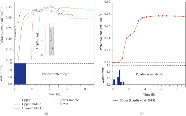
Figure 6: Comparison of wetting front progression versus time as derived from (a) second infiltration test of this study measured by electrical resistance sensors and (b) modified from Hardie et al. [19]. The ponded water depth at the upper boundary is also indicated.

is found adequate. Consequently, they have been used as reference to evaluate the impacts of different methods for determining soil hydraulic properties on modeling results.

3.3. Water Content and Water Flux Observations. As

men-tioned in the setup section, a second infiltration experiment was performed to obtain information about the advancement of the wetting front in the column test. In this test, a

constant infiltration of ponded water was maintained at 3 mm during 75 min and then the column was drained for 8 h to measure the water content and water flow profiles. The bottom boundary condition was a free draining condition allowing free outflow when saturation occurs at the bottom. Under these conditions, a comparison of the wetting front progression versus time is presented in Figure 6, which show water content measured by electrical resistance sensors

(9)

installed in the soil column. In this scenario, a wetting front example modified from Hardie et al. [19] is also presented for comparison.

As shown in this figure, the results indicate that water content near the top of the column increased sharply during the infiltration test and decreased shortly after the ponded infiltration was stopped, while the water content for the lower portion of the soil column increased and decreased at a delayed time and at a slower rate as compared with those for the upper section. Based on these data, the top sensor exhibits water content increment in 8 min after the beginning of the test. Thus, when the top probe detects a 13% of water content, the middle-up sensor detects the wetting front 15 min after the test began. These wetting fronts are very similar to those reported by Hardie et al. [19] (Figure 6(b)), who found that flow paths depend on the soil’s wettability that is dynamically changing with the actual dynamics of soil water content. Nevertheless, the use of capacitance based soil moisture monitoring may however be limited in soils in which macropore flow is enhanced at high antecedent soil moisture content. Hence, the differences in terms of magnitude and shape between both results could be due to differences in water content monitoring, boundary conditions at the upper boundary, and porous media features. The electrical resistance probes without a gypsum block were also used to detect drainage processes in the automated test column (ATC). As a result, the peak values of each curve occurred about one hour after the waterfront was detected. After each peak, the electrical resistance increases as a result of a slight water content decrement on the upper and upper-middle sensors. Although the response of the probe inside the gypsum block (Figure 6(a)) is consistent with the other probes in the wetting stage, the drainage response presents a slight delay compared to the sensor response without a gypsum block. For this test, after 56 hours of the column test it reached the same steady-state value as the others sensors. As mentioned earlier, one advantage of covering the electrical resistance sensors with gypsum blocks is to provide more stability between readings in soils with different salinity degree, whereas a disadvantage is a delayed drainage response. One advantage of using electrical resistance probes without a gypsum block is their fast response in transient state; however, they must be calibrated individually for each type of soil. According to the experimental purposes of the investigation, in which the ATC may be used, it is also suggested that users need to decide which type of electrical resistance probe is more sensitive and suitable for a reasonable estimate.

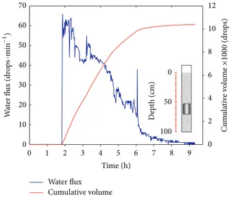
On the other hand, Figure 7 depicts the drop counter readings with a fixed 1 min sample rate, which shows the water flux and cumulative volume measured by the sensor during the second infiltration test. On the left axis, the flow rate is expressed in drops⋅min−1_{, while, on the right axis, it} is expressed as cumulative volume in drops. Initially, there is virtually no flow registered by the instrument into the soil column under partially saturated conditions. In this schema, Figure 7 shows that, after 1.8 h from the start of the test, the water flux increases above the retention capacity of the

0 10 20 30 40 50 60 70 W at er ﬂ ux (dr o p s· min −1 ) 0 1 2 3 4 5 6 7 8 9 Time (h) 0 2 4 6 8 10 12 C u m u la ti ve volu me × 1000 (dr o p s) Water ﬂux Cumulative volume D ep th (cm) 0 50 100

Figure 7: Graph of the vertical water flow and cumulative volume measured in the drop counter during the second infiltration test.

porous media and water begins to flow through the drop counter, as expected based on capillary theory. In the next hours, two picks of water flux were observed by the sensor and it was followed by a smooth desaturation curve in terms of stationary capillary pressures at the end of the infiltration experiment. The peak that occurred after six hours may possibly be attributed to the spatial variability of soil moisture and/or the degree to which the sensor is in contact with the soil material.

As earlier mentioned, the maximum rate measured by the drop counter is approximately 1190 drops⋅min−1_{, which is} higher than the maximum value registered by the instrument during the test (68 drops⋅min−1). On the basis of this explana-tion, the measured vertical flow rates are in a valid measuring range for all tests. In order to provide a realistic and smooth response, a digital low-flow filter was implemented in the final design of the drop counter output data. Considering this stage, the graph of the cumulative volume shows the filtered data of the water flow rate, resulting in an associated smooth curve. It should be noted, however, although the magnitudes of the flow rates remain similar despite the fact that the peaks are not considered, the data collection of this system does not significantly vary over the sampled time interval.

3.4. Comparison of Simulated and Measured Water Content and Water Flux Profiles. Results obtained from a

combi-nation of direct and indirect methods, to estimate the soil physical characteristics, were then used to simulate soil moisture and water flow evolution. The parameter sets of the van Genuchten equations for the soil column tests are given in Table 1. The Hydrus-1D model was run with the different parameter sets to simulate water content and water flow during the redistribution phase, assuming one-dimensional water flow in variable saturated porous media. Simulated and measured water contents were then compared and differences were quantified with the statistical performance criteria defined earlier. Figure 8 shows, as an example, the

(10)

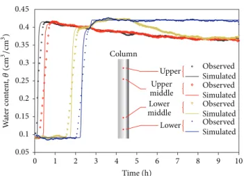
0 1 2 3 4 5 6 7 8 9 10 Time (h) 0.05 0.1 0.15 0.2 0.25 0.3 0.35 0.4 0.45 W at er co n ten t, 𝜃( cm 3/ cm 3) Observed Simulated Observed Simulated Observed Simulated Observed Simulated Upper Column Upper middle Lower middle Lower

Figure 8: Performance comparison between the water content observed in the electrical resistivity probes and the water content simulated by Hydrus-1D model. The results correspond to the third infiltration test for a time period of ten hours.

water content profiles simulated and observed 10 h after the beginning of the column experiment.

Under the conditions simulated, the results show that the water content, measured in the upper and the upper-middle resistivity sensors, increased sharply during the infiltration test and decreased asymptotically approaching steady-state values near the end of the event. In this scenario, the lower portion of the column test (lower sensor) increased and decreased at a delayed time and decreased to reach the same steady-state condition as compared with those of the upper portion. Moreover, as it is indicated in Figure 8, the distribution of the water content, measured by the lower middle sensor, resulted in a slightly increased water content compared to the other estimations. According to Cey et al. [43], the flow system response will become increasingly sensitive as soil moisture approaches saturation. The degree of sensitivity will obviously depend on the shape of the soil water retention curve, soil layering, and the history of prior infiltration events.

Regarding the statistical analysis results, the fit indi-cators averages of the simulated water content compared to the observed readings from the resistance probes give satisfactory results, with ME = 0.1028 cm3⋅cm−3, RMSE = 0.01412 cm3⋅cm−3, 𝑅2 = 0.9080, EF = 0.9377, and CRM = −0.0009. In this analysis, the ME, RMSE, and CRM values obtained were close to zero, indicating that the simulated values reasonably match with the observed ones. In addition, the CRM value obtained indicates a slight tendency in the model to overestimate the observed values of water content, but this tendency is not very strong because all CRM values are around zero. Low values of RMSE also indicated the applicability of Hydrus-1D to simulate the soil hydraulic functions and water fluxes in the column experiment. Hence, it could be concluded that these identification results were similar in reliability to those obtained in various studies using TDR and tensiometer measurements to estimate the hydraulic parameters. Jacques et al. [44] found RMSE values

ranging within 0.038–0.125 cm3cm−3 for the measured and simulated water contents. In other studies that carried out the validation of an agroecosystem model that also used TDR measurements, RMSE values varied in the range of 0.010– 0.035 cm3cm−3 in the study of Heidmann et al. [45] and in the range of 0.03–0.130 cm3cm−3in the study of Wegehenkel [46].

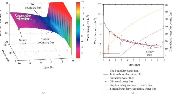
Figure 9 summarizes results of the simulated and observed water fluxes, 𝑞, in a transient state versus depth and time, including also the boundary conditions with input parameters listed in Table 1. In Figure 9(a), these variables are identified in a 3D graph, which indicates their global response in transient state, as well as the flow rates estimated in the drop counter. Figure 9(b) outlines the same curves in a 2D graph (left axis) and the cumulative water fluxes measured in the drop counter (identified as circles) and simulated by Hydrus-1D (right axis). Based on the modeling results, the flow rates measured in the drop counter showed good agreement with the flow rates simulated by the Hydrus-1D model. The differences between modeled and measured values may be caused by applied averaging data of atmo-spheric boundary condition or by the possible existence of preferential flow paths in the soil. It is important to point out that the drop counter observed values were not used in the model calibration; thereby, they constitute an independent verification of the model.

In a broad sense, the total cost estimated of the ATC is under US$ 400, which represents a low-cost compared to available commercial instruments that perform similar functions. In such a context, the HOBO Micro Station Data Logger (model H21-002, [47]), which was not included in this study, is capable of collecting and storing data from the four sensors, at an approximate cost of US$ 231. Addi-tionally, if the price of five commercial electrical resistivity cells is considered, at US$ 120 each (model 2731312-31S-24T OAKTON, [48]), the total cost reaches US$ 831, twice the cost of the devices installed in the ATC used in this study, which support the capability of this low-cost monitoring system. This estimation just includes the data-logger and the electrical resistivity probes without considering the price of the tensiometers and the mechanical structure of the ATC.

4. Summary and Conclusions

In many numerical simulations that include the vadose zone, it is common practice to estimate unsaturated soil hydraulic properties because they are either too expensive or too difficult to measure directly. Nevertheless, the reliability of these parameters should be scrutinized, because estimations are based on general data sets, and verification with true field data is often lacking. Considering this fact, an automated test column (ATC) was developed to measure automated long-term soil water content, matric potential, and water fluxes through a homogeneous unsaturated porous medium. A combination of direct and indirect methods approaches were used to estimate soil hydraulic parameters and demonstrated their suitability in a one-dimensional model (Hydrus-1D) to simulate transient infiltration through partially saturated soils.

(11)

10 8 6 4 2 0 20 15 10 5 0 W at er fl ux, q (cm ·h − 1) D ep_{th (cm)} Time (h) 2 4 6 8 10 12 14 16 18 20 W at er fl ux, q (cm ·h − 1 ) Steady state Bottom boundary flux Top boundary flux 0 50 100 Drop counter water flux (a) 0 1 2 3 4 5 6 7 8 9 10 Time (hr) 0 10 20 30 40 50 60 70 C u m u la ti ve wa ter fl ux den si ty (cm) 0 5 10 15 20 25 W at er fl ux, q( cm ·h − 1) Steady state

Top boundary water flux Bottom boundary water flux Simulated water flux Observed water flux

Top boundary cumulative water ﬂux Bottom boundary cumulative water ﬂux

(b)

Figure 9: Water flux,𝑞, in a transient state as a function of depth and time: (a) water flux simulated in a 3D plot showing upper boundary flow (𝑧 = 0 cm), lower boundary flow (𝑧 = 100 cm), and water flux at bottom of the drop counter (𝑧 = 60 cm); (b) the same curves as in (a) (left axis) and the cumulative water flux measured in the drop counter and simulated by Hydrus-1D (right axis).

Calibrations of electrical resistance probes reasonably match with similar studies, and the differences observed can be attributed to factors in manufacturing process and dimensions. The maximum errors of calibration of the ten-siometers were 3.2% and 4.6% in respect to the full range, which represent slight differences between simulated and measured values of the voltage response. The sensors were found to be stable once calibrated and required maintenance or recalibration is not needed to estimate the soil hydrody-namics parameters in partially saturated soil environments. Data measured by the drop counter installed in the ATC exhibited a high consistency with the electrical resistance probes during the infiltration tests that showed the ATC capabilities; thus the output model was compared favorably with the water flow rates measured by the sensor. The drop counter provides an independent verification of the model and indicates an evaluation of water mass balance to be identified with confidence.

Results of the statistical analyses showed good perfor-mance of the model for the infiltration tests, which suggests a robustness of the methodology developed in this study, especially for the lower middle and lower sensors. This indicates that the hydrodynamic model used to simulate the water flow in this homogeneous sand column is quite appropriate. Some differences appear due possibly to a hysteresis effect during the drainage phase and variability within the soil column. The three major advantages of these sensors for examination of flow dynamics monitoring under partially saturated conditions are as follows: (1) allowing data acquisition at any specified time interval;(2) providing

potentially more accurate data by minimizing disturbance of subsurface conditions; and (3) minimizing the cost of electronic components and laboratory procedures involved in sample retrieval and analysis.

The cost of the ATC is less than US$ 400, a very low cost compared to industrial sensor technologies with sim-ilar functions. The system contains low-cost commercially available components and proved durable over the course of nearly 3 years of operation. For high or low water tempera-ture applications, an additional calibration of the resistance probes of the ATC may be required. As an extension to the applicability of this system, the low-cost system described herein, including some modifications, could be applied to low-budget projects, which may require the monitoring of either in situ hydraulic properties of the vadose zone or chemical changes of infiltrating water in the subsurface, which may be correlated with resistivity changes.

Competing Interests

The authors declare that they have no competing interests.

Acknowledgments

The authors would like to acknowledge the Ministère des Relations Internationales du Québec, the Consejo Nacional de Ciencia y Tecnolog´ıa (CONACyT 201800), the Consejo Mexiquense de Ciencia y Tecnolog´ıa (COMECYT), the Universidad Autónoma del Estado de México (UAEM), the Institut National de la Recherche Scientifique (INRS-ETE),

(12)

and the Ministère d’Éducation du Québec for providing funding and logistical support for this study. The authors are also grateful for the technical support of the laboratory tech-nicians from the Inter-American Centre of Water Resources (CIRA) in Toluca, Mexico.

References

[1] National Research Council, Soil and Water Quality; An Agenda

for Agriculture, National Academic Press, Washington, DC,

USA, 1993.

[2] H. Lin, “Hydropedology: bridging disciplines, scales and data,”

Vadose Zone Journal, vol. 2, no. 1, pp. 1–11, 2003.

[3] R. Angulo-Jaramillo, J.-P. Vandervaere, S. Roulier, J.-L. Thony, J.-P. Gaudet, and M. Vauclin, “Field measurement of soil surface hydraulic properties by disc and ring infiltrometers. A review and recent developments,” Soil and Tillage Research, vol. 55, no. 1-2, pp. 1–29, 2000.

[4] J. Mertens, H. Madsen, L. Feyen, D. Jacques, and J. Feyen, “Including prior information in the estimation of effective soil parameters in unsaturated zone modelling,” Journal of

Hydrology, vol. 294, no. 4, pp. 251–269, 2004.

[5] M. Mollerup, S. Hansen, C. Petersen, and J. H. Kjaersgaard, “A MATLAB program for estimation of unsaturated hydraulic soil parameters using an infiltrometer technique,” Computers and

Geosciences, vol. 34, no. 8, pp. 861–875, 2008.

[6] M. M. Gribb, I. Forkutsa, A. Hansen, D. G. Chandler, and J. P. McNamara, “The effect of various soil hydraulic property estimates on soil moisture simulations,” Vadose Zone Journal, vol. 8, no. 2, pp. 321–331, 2009.

[7] T. P. A. Ferr´e and G. Kluitenberg, “Advances in monitoring and measurement methods: preface from the guest editors,” Vadose

Zone Journal, vol. 2, article 443, 2003.

[8] M. D. Madsen and D. G. Chandler, “Automation and use of mini disk infiltrometers,” Soil Science Society of America Journal, vol. 71, no. 5, pp. 1469–1472, 2007.

[9] F. Masrouri, K. V. Bicalho, and K. Kawai, “Laboratory hydraulic testing in unsaturated soils,” Geotechnical and Geological

Engi-neering, vol. 26, no. 6, pp. 691–704, 2008.

[10] S. A. Al Hagrey, T. Schubert-Klempnauer, D. Wachsmuth, J. Michaelsen, and R. Meissner, “Preferential flow: first results of a full-scale flow model,” Geophysical Journal International, vol. 138, no. 3, pp. 643–654, 1999.

[11] B. Ahrenholz, J. T¨olke, P. Lehmann et al., “Prediction of cap-illary hysteresis in a porous material using lattice-Boltzmann methods and comparison to experimental data and a morpho-logical pore network model,” Advances in Water Resources, vol. 31, no. 9, pp. 1151–1173, 2008.

[12] L. A. Richards, “Capillary conduction of liquids through porous mediums,” Journal of Applied Physics, vol. 1, no. 5, pp. 318–333, 1931.

[13] D. W. Zachmann, P. C. DuChateau, and A. Klute, “The cali-bration of the richards flow equation for a draining column by parameter identification,” Soil Science Society of America

Journal, vol. 45, no. 6, pp. 1012–1015, 1981.

[14] J. C. Parker, J. B. Kool, and M. T. Genuchten, “Determining soil hydraulic properties from one-step outflow experiments by parameter estimation: II. Experimental studies,” Soil Science

Society of America Journal, vol. 49, no. 6, pp. 1354–1359, 1985.

[15] D. Russo, E. Bresler, U. Shani, and J. C. Parker, “Analyses of infiltration events in relation to determining soil hydraulic

properties by inverse problem methodology,” Water Resources

Research, vol. 27, no. 6, pp. 1361–1373, 1991.

[16] J. ˇSim˚unek and M. T. van Genuchten, “Estimating unsaturated soil hydraulic properties from tension disc infiltrometer data by numerical inversion,” Water Resources Research, vol. 32, no. 9, pp. 2683–2696, 1996.

[17] M. T. van Genuchten, “Closed-form equation for predicting the hydraulic conductivity of unsaturated soils,” Soil Science Society

of America Journal, vol. 44, no. 5, pp. 892–898, 1980.

[18] R. F. Carsel and R. S. Parrish, “Developing joint probability distributions of soil water retention characteristics,” Water

Resources Research, vol. 24, no. 5, pp. 755–769, 1988.

[19] M. Hardie, S. Lisson, R. Doyle, and W. Cotching, “Determining the frequency, depth and velocity of preferential flow by high frequency soil moisture monitoring,” Journal of Contaminant

Hydrology, vol. 144, pp. 66–77, 2013.

[20] A. Ritter, R. Mu˜noz-Carpena, C. M. Regalado, M. Vanclooster, and S. Lambot, “Analysis of alternative measurement strategies for the inverse optimization of the hydraulic properties of a volcanic soil,” Journal of Hydrology, vol. 295, no. 1-4, pp. 124– 139, 2004.

[21] P. Scholl, D. Leitner, G. Kammerer, W. Loiskandl, H.-P. Kaul, and G. Bodner, “Root induced changes of effective 1D hydraulic properties in a soil column,” Plant and Soil, vol. 381, no. 1, pp. 193–213, 2014.

[22] A. Skinner, C. Hignett, and J. Dearden, Resurrecting the Gypsum

Block for Soil Moisture Measurement, Australian Viticulture,

1997.

[23] R. J. Tocci and N. S. Widmer, Digital Systems: Principles and

Applications, Prentice Hall, Upper Saddle River, NJ, USA, 8th

edition, 2001.

[24] “Freescale semiconductor integrated silicon pressure sensor on-chip signal conditioned,” Data Sheet. Review 11, 2010.

[25] Microchip Technology, “PIC18F2455/2550/4455/4550 data sheet. 28/40/44-Pin, high performance, enhanced flash, USB micro-controllers with nanoWatt technology,” Data Sheet. Document DS39632, Microchip Technology, 2007.

[26] L. Sanders, A Manual of Field Hydrogeology, Edited by P. Hall, Prentice-Hall, Upper Saddle River, NJ, USA, 1998.

[27] R. Kuechler, K. Noack, and T. Zorn, “Investigation of gypsum dissolution under saturated and unsaturated water conditions,”

Ecological Modelling, vol. 176, no. 1-2, pp. 1–14, 2004.

[28] USDA, Soil Survey Laboratory Methods Manual. Soil Survey

Laboratory Investigations Report, United States Department of

Agriculture, Natural Resources Conservation Service, 2004. [29] R. J. Bathurst, A. F. Ho, and G. Siemens, “A column apparatus

for investigation of 1-D unsaturated-saturated response of sand-geotextile systems,” Geotechnical Testing Journal, vol. 30, no. 6, pp. 433–441, 2007.

[30] J. ˇSim˚unek and M. T. Van Genuchten, “Modeling nonequilib-rium flow and transport processes using HYDRUS,” Vadose

Zone Journal, vol. 7, no. 2, pp. 782–797, 2008.

[31] L. Wissmeier and D. A. Barry, “Reactive transport in unsat-urated soil: comprehensive modelling of the dynamic spatial and temporal mass balance of water and chemical components,”

Advances in Water Resources, vol. 31, no. 5, pp. 858–875, 2008.

[32] E. L´eger, A. Saintenoy, and Y. Coquet, “Hydrodynamic param-eters of a sandy soil determined by ground-penetrating radar inside a single ring infiltrometer,” Water Resources Research, vol. 50, no. 7, pp. 5459–5474, 2014.

(13)

[33] M. G. Schaap, F. J. Leij, and M. T. van Genuchten, “A bootstrapneural network approach to predict soil hydraulic parameters,” in Proceedings of the International Workshop on

Characterization and Measurements of the Hydraulic Properties of Unsaturated Porous Media, M. T. van Genuchten and F. J. Leij,

Eds., University of California, Riverside, Calif, USA, 1999. [34] A. Klute, “Water retention: laboratory methods,” in Methods of

Soil Analysis. I. Physical and Mineralogical Methods, C. A. Black,

Ed., Soil Science Society of America Book Series, pp. 635–662, Soil Science Society of America, Madison, Wis, USA, 1986. [35] T. J. Kelleners, D. A. Robinson, P. J. Shouse, J. E. Ayars, and T.

H. Skaggs, “Frequency dependence of the complex permittivity and its impact on dielectric sensor calibration in soils,” Soil

Science Society of America Journal, vol. 69, no. 1, pp. 67–76, 2005.

[36] T. Sander and H. H. Gerke, “Modelling field-data of preferential flow in paddy soil induced by earthworm burrows,” Journal of

Contaminant Hydrology, vol. 104, no. 1–4, pp. 126–136, 2009.

[37] N. Islam, W. W. Wallender, J. P. Mitchell, S. Wicks, and R. E. Howitt, “Performance evaluation of methods for the estimation of soil hydraulic parameters and their suitability in a hydrologic model,” Geoderma, vol. 134, no. 1-2, pp. 135–151, 2006. [38] Y. Mualem, “A new model for predicting the hydraulic

conduc-tivity of unsaturated porous media,” Water Resources Research, vol. 12, no. 3, pp. 513–522, 1976.

[39] M. Homaee, C. Dirksen, and R. A. Feddes, “Simulation of root water uptake: I. Non-uniform transient salinity using different macroscopic reduction functions,” Agricultural Water

Manage-ment, vol. 57, no. 2, pp. 89–109, 2002.

[40] J. Salas-Garc´ıa, Determinaci´on espacial de la recarga mediante el

diseño e instalación de instrumentación en pozos de monitoreo y simulación de la infiltración en la zona vadosa [Tesis doctoral],

Centro Interamericano de Recursos del Agua (CIRA), Univer-sidad Autónoma del Estado de México, Toluca, México, 2012. [41] G. B. Paige and D. Hillel, “Comparison of three methods for

assessing soil hydraulic properties,” Soil Science, vol. 155, no. 3, pp. 175–189, 1993.

[42] A. Mermoud and D. Xu, “Comparative analysis of three meth-ods to generate soil hydraulic functions,” Soil and Tillage

Re-search, vol. 87, no. 1, pp. 89–100, 2006.

[43] E. Cey, D. Rudolph, and R. Therrien, “Simulation of ground-water recharge dynamics in partially saturated fractured soils incorporating spatially variable fracture apertures,” Water

Resources Research, vol. 42, no. 9, Article ID W09413, 2006.

[44] D. Jacques, J. ˇSim˚unek, A. Timmerman, and J. Feyen, “Calibra-tion of Richards’ and convec“Calibra-tion-dispersion equa“Calibra-tions to field-scale water flow and solute transport under rainfall conditions,”

Journal of Hydrology, vol. 259, no. 1–4, pp. 15–31, 2002.

[45] T. Heidmann, A. Thomsen, and K. Schelde, “Modelling soil water dynamics in winter wheat using different estimates of canopy development,” Ecological Modelling, vol. 129, no. 2-3, pp. 229–243, 2000.

[46] M. Wegehenkel, “Validation of a soil water balance model using soil water content and pressure head data,” Hydrological

Processes, vol. 19, no. 6, pp. 1139–1164, 2005.

[47] ONSET, HOBO Micro Station Data Logger-H21-002, Product specifications, 2015, http://www.onsetcomp.com/products/data-loggers/h21-002.

[48] Cole-Parmer, 2731312-31S-24T OAKTON. Conductivity Cell, K=1.0, Epoxy, Dip-Style, 100 Ohm Pt RTD ATC, 2015, http:// www.coleparmer.com/buy/product/83345-conductivity-cell-k-1-0-epoxy-dip-style-100-ohm-pt-rtd-atc-2731312-31s-oakton .html.

(14)

Submit your manuscripts at

https://www.hindawi.com

Hindawi Publishing Corporation

http://www.hindawi.com Volume 2014

Climatology

Journal of

Ecology

Earthquakes

Journal of Hindawi Publishing Corporation

Hindawi Publishing Corporation http://www.hindawi.com

Applied &

Environmental

Soil Science

Volume 2014

Mining

http://www.hindawi.com Volume 2014 International Journal of

Geophysics

Oceanography

International Journal of Hindawi Publishing Corporation

Journal of Computational Environmental Sciences

http://www.hindawi.com Volume 2014 Journal of

Petroleum Engineering

Geochemistry

Journal of

Atmospheric Sciences

International Journal of

Oceanography

Advances in

Mineralogy

International Journal of

Meteorology

Advances in

The Scientific

World Journal

Paleontology Journal Hindawi Publishing Corporation

Scientifica

http://www.hindawi.com Volume 2014 Geological ResearchJournal of