OATAO is an open access repository that collects the work of Toulouse
researchers and makes it freely available over the web where possible
Any correspondence concerning this service should be sent
to the repository administrator:
[email protected]
This is an author’s version published in: http://oatao.univ-toulouse.fr/25667
To cite this version:
Amirdehi, Saba and Trajin, Baptiste
and Vidal, Paul-Etienne
and Vally, Johana and Colin, Didier Power transformer model in
railway applications based on bond graph and parameter
identification. (2020) IEEE Transactions on Transportation
Electrification. ISSN 2332-7782
Official URL:
https://doi.org/10.1109/TTE.2020.2979598
Abstract—Validation and verification are the most important issues in railway applications due to cost and security reasons. Therefore, having a model of the system would be necessary in this case. Due to non-ideal test conditions in industrial applications, an accurate parameter identification process has to be defined. In this paper, bond graph method is used to model energy exchanges within components of a traction chain. More precisely, the non-linear transformer model and its parameter identification is studied. In the case of non-ideal test conditions, the usual Jiles-Atherton parameter identification procedure can not be performed. Regarding state of the art, the Jiles-Atherton parameter identification is discussed. It is highlighted that an uncomplete hysteresis cycle, including extremum point and coercive field are mandatory for an accurate parameter identification. The proposed identification process is applied to a real application case. The obtained parameters are then inserted into the overall system model. The consecutive simulations are compared to experimental data obtained through traction chain test bench.
Index Terms— Power transformer simulation, Parameters identification, hysteresis cycle, Traction chain
I. INTRODUCTION
n railway conversion chain design, validation and verification are the most important issues due to costs and security reasons. Power transformers are one of the most expensive components in railway traction systems. In order to reduce costs, having an accurate simulation model of this component is necessary. This model is then used in a simulation process to test several risk occurrences, previously to verification procedures. The simulated model should consist of physical phenomena considering exchanged energies. To be implemented in real time simulators as a part of a whole traction chain, the transformer model should be simple enough as well. The simulation parameters are determined using experimental results in ideal conditions. Those results are often used to validate the simulation results. Nevertheless, in industrial applications, it is not easy to have an ideal test condition due to nonlinear sensors for measurements, non-ideal environment condition and effect of other parts of traction chain. Moreover, the accurate model is not often provided by transformer
designer. As a matter of fact, in high power transport applications it is important to be able to model and identify the model parameters on the real component. This allows having simulation results close to real experiments.
In many previous studies, non-ideal transformer model was proposed [1]- [2]. In [3], the mathematical analysis and modelling of the transformer is presented based on Kirchhoff law by neglecting the influence of leakage flux and hysteresis behavior of magnetizing inductance. These approaches allow to establish equivalent electrical circuit model. Nevertheless, these models do not express inner electromagnetic nonlinear phenomena. Therefore, it is necessary to obtain a model of transformer that includes nonlinear characteristics (hysteresis) of magnetic core [4].
There are different mathematical models to reproduce the hysteresis characteristics of magnetic components [5]- [6]. Among them, Jiles-Atherton (JA) model [7] is the most accurate and precise description of hysteresis characteristics [8], [9] of iron losses for power transformers. To address the previous drawback, numerical simulations of single-phase transformer using inaccurate characterization of Jiles-Atherton (JA) model is proposed in [10] based on the finite element method. Some studies established a link between the finite elements (FEM) method and JA model for parameter identification [11]. But the integration of FEM method into a dynamic and time dependent simulation of a system is difficult to achieve.
In [12], the transformer model based on Transmission Line Model (TLM) is proposed using an accurate characterization of JA model. However, characteristics and effects of substation and catenary are necessary in our case but are not associated with non-linear transformer model in previous literature. In this paper, the innovation is to accurately model the transformer nonlinearities as a part of the whole input part of the traction chain. Using the complete model of input power chain let us simulate its behavior in different conditions such as steady state and transient.
To identify the parameters of JA model, it is needed to have experimental hysteresis characteristics. In last few years, different methods of parameter identification for JA model have been proposed. The traditional and known method is numerical determination as proposed in [13]. In [14], random and deterministic searches were done to perform the identification. False position method is used in [15] as a new method of
Power transformer model in railway
applications based on bond graph and parameter
identification
Amirdehi S., Trajin B., Vidal P.-E., Vally J. and Colin D.
parameter estimations for JA model. In [16] an alternative approach based on ‘‘branch and bound’’ optimization method is explained. A robust method to determine numerically the Jiles-Atherton model parameters is presented in [17]. These parameter estimations require no load test of transformer with an ideal test condition to have the complete hysteresis loop. Some of the studies use the data sheet information. These test procedures are not easy to do in railway applications. Effectively, the presence of all traction chain or non-ideal sensors during the test may alter the complete hysteresis loop monitoring. Therefore, it is important to do the analysis on parameter estimation when the whole ! " # hysteresis cycle cannot be provided. This is the purpose of one section of the paper.
In this paper, a complete input power of a railway traction chain including nonlinear transformer is modeled based on bond graph methodology. It allows a specific writing of JA equations that can be inserted into state equations of the whole system. Consequently, JA model can be easily solved by a real time simulator using numerical integrations methods. The JA model is used to model the hysteresis loop. All state equations of the system are obtained directly from bond graph. In order to estimate the JA parameters in the case of non-ideal test condition, specific analysis is done on parameter identification just by part of a hysteresis cycle.
The paper is organized as follows. In section II, the complete traction chain model, including the transformer is proposed. It is based on a bond graph with integral causality. The load connected to the secondary will be modelled ideally. All state equations achieved by the bond graph analysis are provided. It includes the new representation of JA model. In section III, the magnetizing current simulated by JA model is presented in detail. In section IV, the analyses of parameter identifications are done on entire and uncomplete hysteresis loop. In section V, railway experimental results are compared with simulation results using the parameters obtained by uncomplete hysteresis loop.
II. DESCRIPTION OF THE TRANSFORMER MODEL
A. Input Power Model
Nonlinear transformer models have been proposed in literature [1]- [2]. Let us remark that during energization the transformer experiences a flux that may reach up to twice its nominal steady state value [18], [19]. However, this phenomenon is not taken into account in this paper. The electromagnetic circuit models are accurate and complete enough to do the simulation in our case [20], [2]. As illustrated in Fig.1, the input ideal voltage source $%(&), the substation, the catenary and the transformer are taken into account in the traction chain model. Some details on their model are given in the following.
Fig. 1. Input power of traction chain including substation, catenary and non-ideal transformer
Fig.1 represents input power of traction chain with single phase transformer with resistance and inductance leakage in primary winding, '*, +* respectively.'-, +. in the shunt branch, represent the core behavior including nonlinearity, saturation and hysteresis, and eddy current phenomena. '/0, +/0,'/1and +/1represent leakage resistance and inductance of two windings in secondary part respectively. '2 and +2 represent resistance and inductance of substation respectively. The change in distance between train and substation are modeled through the variation of ∏ model of catenary parameters '345,63450,63451and +345[21].
In section II.B, the bond graph representation with integral causality which allows to establish the state equations is detailed.
B. Bond Graph of Whole System
The method of bond graph [22] allows representing in a graphic way power transfers in systems. Elements are connected to each other by considering oriented exchange links supporting generalized efforts and flows and junctions [22], [23]. Fig. 2 shows the bond graph of whole traction chain considered in Fig. 1.
Fig. 2. Bond graph of input power of traction chain including substation, catenary and non-ideal transformer
Based on the causality analysis of generalized variables, state equations of the whole system are established in the following.
C. State Equations based on Bond Graph
Considering all energy variables and causalities illustrated in Fig. 2, state equations and variables are easily obtained (1)-(8). The state variables are 7/89(&), 7345(&), $345:(&), $345;(&), 7*(&), 7/:(&),<7/;(&) and 7.(&) and they are highlighted in red in Fig. 2. The primary side of transformer contains the nonlinear magnetizing inductance.
7=/89(&) >"'2+2 7/89(&) "+2? $345:(&) @+2? $%(&) (1) $=345:(&) >6345:? 7/89(&) "6345:? 7345(&) (2) 7=345(&) >"'345+345 7345(&) @+345? $345:(&) "+345? $345;(&) (3) $=345;(&) >6345;? 7345(&) "6345;? 7*(&) (4) 7=*(&) >$345;(&)+* "'*+*7*(&) "$2(&)+* (5) State equations in secondary part of transformer are such as:
7=/0(&) >A"'/07/:(t) @ B:$2(t)<" $/0+/: (t)C (6) 7=/1(&) > D"'/17/;(t) @ B;$2(t) " $/1(t)E +/; (7)
where in (6)-(8), $2(&) is:
$2(&) > '-(7F(&) " B:7/:(&) " B;7/;(&) " 7.(&)) (8) Consequently, inputs of the system are voltage of substation $%(&) and voltage sources in the two secondary windings $/:(t), $/;(t). To complete the set of state equations, it is required to express the derivative of the magnetizing current 7=.(&) using magnetic relations in core and state variables.
III. MAGNETIZING CURRENT USING JA MODEL
A. Magnetic Core Equations
The magnetizing current 7.(&) in single-phase transformers is calculated using the magnetic flux (G.), the magnetic core field (#), magnetic induction (!) and magnetization (H). Taking into account the voltage of magnetizing branch $2(&) and number of turn in primary winding I, the magnetic flux will be as (9):
G=.(&) > "$2(&)I J (9) The magnetic induction can be expressed using Faraday’s law as below:
!=(&) > "$2IK ,(&) (10) where K is the cross-section area of the primary winding supposing that ! is constant within the whole cross-section area.
The three fundamental magnetic terms can be related such as: !(&) > LM(#(&) @ H(&))J< (11) For simplicity purpose, in the following, the time dependence of !, #, H and 7. will not be mentioned in the following expressions.
Considering the relation between magnetic field and magnetization [24], (12) is achieved by derivative of (11).
N!
N& > LMON#N& @NHN& P > LMN#N& O? @NHN#PJ< (12) Based on Ampere theorem (13), magnetizing current 7.(&) can be obtain once magnetic field is achieved.
7.(&) > #(&)JIJQ (13)
Therefore, by substitution of (9), (10) and (13) in (12), magnetizing current equation will be as (14).
7=.(&) >$2(&)+. > QJ $2(&) I;KLMD? @ NH
N#E
J (14)
where +. is a nonlinear magnetizing inductance and Q is the average magnetic path.
As it is shown in (14), derivative of the magnetizing current 7. depends on RSRT. This term can be obtained by JA model and its five parameters as detailed in the following section.
B. Calculation of dM/dH Using JA Model
The nonlinear characteristic of hysteresis loop (B-H curve) can be determined by the mathematical model which was developed by Jiles and Atherton [14, 23]. This mathematical model is based on physical considerations. The model is defined by a simple first order differential equation and characterized by five parameters. Based on this theory, the magnetization decomposes into a reversible component HUVW and an irreversible component HXUU.
H > HUVW@ HXUUJ (15)
In ferromagnetic materials, the effective field #V is the interaction between magnetic moments which is defined as below:
#V> # @ YH, (16)
where Y is the Weiss correction factor that represents the coupling between fields. Anhysteretic curve is the average of ascending and descending parts of the major hysteresis loop, namely, H4Z. It can be obtained by Langevin function [25], and is such as: H4Z(#V) > H/45[\]&^ DT_ 4E " D 4 T_E`, (17)
where a and H/45 are shape factor and saturation magnetization, respectively.<HUVW has a relation with anhysteretic magnetization and irreversible component of magnetization by a reversibility coefficient \ which depends on material nature as below:
HUVW> \(H4Z" HXUU)J (18) The differential equation associated with irreversible magnetization component is defined by [7]:
NHXUU
N# >cb " Y(H4Zb.(H4Z" HXUU)" HXUU)J
(19)
Where c is the Boltmann constant which is linked to coercive field and the factor of b.and b are as below:
b.> d e f e
g?h<<ijN#N& k l<amN<H4Zk HXUU ?h ijN#N& n l<amN<H4Zn HXUU lh ]&^opqiro<<<<<<<<<<<<<<<<<<<<<<<<<<<<<< , (20) b > s?h N# N& k l "?hN#N& n lJ (21)
Using (15) and (18), magnetization is obtained based on irreversible magnetization and anhysteretic magnetization as:
H > (? " \)HXUU@ \H4ZJ (22) Then, the differential equation of RSRT is obtained by derivate of (22). Some mathematical formulation on (19) and (17) are used such as RSRTis:
NH
N# > \NH4ZN# @ (? " \)NHXUUN# J (23) Several approaches proposed different expressions to calculate RS
RTbased on (15)-(22).
However, in order to ease an implementation in real time simulator, it is required to have fewer differential equations and avoid algebraic loop. Our objective in this paper is to propose a new expression of RSRTindependent of HXUUbut only dependent of state variables. By reforming (22), irreversible magnetization is defined as:
HXUU>H " \H4Z? " \ J (24) Therefore, the differential equation associated with irreversible magnetization is:
NHXUU
N# >(? " \) Ocb " Y(Hb.(H4Z" H)4Z" H) ? " \ P
J (25)
Then, the differential equation of anhysteretic magnetization based on magnetic field will be as equation (26):
NH4Z
N# >NH4ZN#V N#VN# J
(26)
Considering equation (16), the differential of anhysteretic magnetization is established as:
NH4Z N# >NH4ZN#V N(# @ YH)N# >NH4ZN#V< <<O? @ YNHN#P, (27) where NH4Z N#V <>a O? " uvtw;H/45D#V a E " D#VaE ; PJ (28)
Finally, the differential of magnetization is rewritten as given in (29). NH N# > \NH4Z N#V @ bbc " Y(H.(H4Z4Z" H)" H) ? " \ ? " Y\NH4Z N#V< J<< (29)
Therefore, as it is discussed in previous section, magnetizing current is calculated using (29). The term RSRT depends on H, H4Zand RSRT_xy. First of all, as shown in (11), H is a function of ! and #. ! is itself a function of state variables through the integration of $2 (8) and (10). # is also a function of a state variable (13). Finally, H4Z and RSRT_xy are functions of #V(17) that is itself a function of #<and H (16) and then a function of state variables.
Equation (30) expresses the magnetizing current as a function of all state variables.
7.= (&) > QJ z'-(7F(&) " B:7/:(&) " B;7/;(&) " 7.(&)){ I;KL
lD?@ NHN#E
J (30) So, all state variables of input power system of our traction chain can be easily calculated using (1)-(8), (30) in sections
II.C, III.A and III.B.
However, to simulate the whole system, it is necessary to identify the five parameters of JA model (Y, c, \, a, H/45) and then to have the hysteresis characteristic of the magnetic core based on experimental results. In section IV., the procedure of parameter identification is done.
IV. IDENTIFICATION OF PARAMETER AND ANALYSIS
A. Example of Hysteresis Loop
To illustrate the use of the JA model and its parameter identification, a first example taken from a previous study is considered [26]. In this previous study, as a first step, a test with a transformer with no load condition is done to obtain the hysteresis characteristics and parameters of JA model. The transformer model with the open secondary is modeled as depicted in Fig.3.
The bond graph method is applied to obtain the state variable and equation. Consequently, the related state equation is:
7.= (&) > $/U3(&)+. "'*7.(&)+. (31) With: +.>I ;KL lD?@ NHN#E Q (32)
In (32), RSRTexpresses as in (29) and depends on state variable using (16), (17), (11), where (10) is replaced by (33).
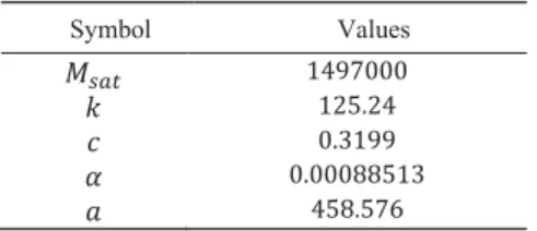
!=(&) > "$/U3(&) " '*7.(&)IK (33) The parameters of electrical circuit and JA are considered based on data provided [26] and summarized in Table I. The simple transformer model is simulated where the magnetizing core characteristics are computed based on (13) and (31)-(33).
In [26],H(#) characteristic of the magnetic material is under concern. However, our proposed modelling methodology based on bond graph and specific writing of JA equations lead us to recover the hysteresis characteristic !(#) in Fig. 4 that is linked to H(#) one.
Fig. 4. Hysteresis loop of transformer with the JA parameters in table I.
Nevertheless, in our railway case study, once the model is established, the identification process is addressed. In parts IV.B and IV.C, parameter identification is done with the entire hysteresis loop and with a percentage of the hysteresis loop. The comparisons between these two study cases are
proposed and discussed in the following.
B. <Identification Process with Complete Hysteresis Loop
As a first step of identification, numerical determination of hysteresis characteristic is used as in [13]. Secondly, Differential Evolution (DE) method [27], [28] is used in order to the parameter fitting for whole hysteresis loop of the transformer. In this case the cost function for DE method is achieved by minimization of the summation of square root of the difference, between desired and calculated signal for every point of hysteresis curve. The cost function is:
| > } ~A(j)•,S" (j)•,€C; •‚‚*
(34)
where<| represent sum of error, (j)•,Sis desired function and (j)•,€is the calculated function by JA model, for each point of the hysteresis loop. The objective is to recover the JA model parameters (Y, c, \, a, H/45) given in Table I. The optimization is started with 500 for number of population and 100 for number of evaluations. As a matter of facts, 50000 number of iterations are applied. The boundary of each parameter is considered between minimum and maximum values in [26]. Table II depicts the selected boundaries for each parameter. Note that as in [26],H/45is constant.
The functions used for optimization process (j)•,S and (j)•,€ are magnetizing current 7.(&). The target error | is set to ensure a relative error on 7.(&) over a period lower than 1%. Table III shows the result of parameter identification for one entire loop of hysteresis.
The values are close to those initially used and given in Table I. That validates the identification method based on DE algorithm. Notice that, initial boundaries for the parameters to identify are required [29] and are detailed in the following.
C. Boundary Setup
Based on [13], the boundaries of JA parameters considering their physical definitions are as following:
TABLE I
TRANSFORMERELECTRICALMAGNETIC PARAMETERS
Symbol Values H/45 ?ƒ„…lll c ?†‡J†ƒ \ lJˆ?„„ Y lJlll‰‰‡?ˆ a ƒ‡‰J‡…Š TABLE II
BOUNDARIES OF JA PARAMETERSUSED IN SIMULATION
Parameters Boundaries c ‹ŒŠ?J†ˆ, ?ˆ‰J…•<Ž c.V4Z± ˆ‰J…• \ ‹ŒlJlƒ‰, lJˆ…ƒ• Ž \.V4Z± ƒˆJ‡•< Y ‹ŒlJlll?Šˆƒ, lJlll„l‰?• ŽY.V4Z± Š„J‡• a ‹Œ?lˆJ†, ƒ…ƒJŠ• Ž a.V4Z± Š‡•< TABLE III
PARAMETERSACHIEVED BY 100%OF A PERIOD
Symbols Differential Evolution
H/45 ?ƒ„…lll
c 126.97
\ 0.32
Y 0.000889
H/45<‹<•H.4‘, ?J†H.4‘’ a<‹<•lJ‡#3, ‡#3’ c<‹<•lJ†#3, ‡#3’ Y<‹< •?l“:M,#.4‘ H.4‘’ \<‹<•l,?’ (35)
To set these boundaries, it is required to have maximum values of magnetization, magnetic field and coercive field. Note that parameters obtained after identification process in section IV.B are included in the boundaries defined in (35).
D. Identification Process with Uncomplete Hysteresis Loop
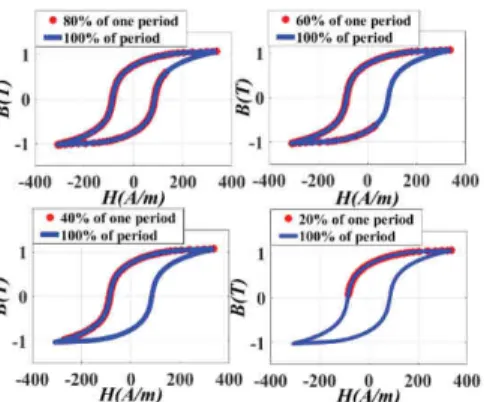
In real transport application, it is sometimes difficult to get the complete hysteresis loop. In the following, different percentages of one hysteresis period from 10% to 100% with a step of 10% are selected. Fig. 5 shows four examples of selected data. The four study cases are: 80%, 60%, 40% and 20% of the entire loop. Note that over a period, signals are constantly sampled regarding time. Every example has the same start point which is (Ba”(#), Ba”(!)).
Fig. 5. Uncomplete hysteresis loop (based on percentage of one period of hysteresis loop 20-40-60-80%)
The identification process of section III.B is repeated for every case of study. The DE parameters (number of evaluations, population and boundaries) are identical. The results are compared to the initial JA parameters shown in Table I. Fig. 6 shows the relative error of parameters for all percentage of hysteresis loop.
Fig. 6. The difference of JA parameters achieved by percentage of period compared to initial JA parameters
It can be observed that the difference between each parameter
achieved by percentage of period and those initially is less than 3%. Note that every percentage from 10% to 100% leads to the same conclusion. It means that in the case of an uncomplete hysteresis cycle, the identification process can be done correctly even if there is only 10% of the hysteresis cycle. Fig.6 highlight the fact that the most sensitive parameter to identification process is k, Fig.6. (c).
To validate the proposed approach, main points in each hysteresis loop are compared to the initial ones. The points chosen are the coercive and remanence points. The initial points are computed based on Fig.4. Fig. 7 illustrates the relative error for coercive (#3), remanence points (!U). In the last curve the error is based on the hysteresis area produced by different percentage of one period of hysteresis loop compared to initial data.
Fig. 7. Relative error for coercive, remanence field and hysteresis area calculated for each hysteresis loop
As depicted in Fig.7, the percentage taken for identification process has low impact on the error made on remanence and coercive fields. Note that the average error of about 0.5% made on overall hysteresis surface remains acceptable. Finally, the sensitivity on parameter k does not have a strong impact on final hysteresis characteristics. Note that, in this case, the start point for identification is the positive extreme value of hysteresis loop. In section III.E, identification processes are done with different start points or different data selection in one period.
E. Identification Process by the Part of a signal period with Different Start Points
In the following, the boundaries defined in section IV.B are considered and used for identification process. In this section, 20% of period is chosen. The impact of different start points as depicted in Fig.8, is studied:
The first and third selections include respectively remanence field !U, and the coercive field #3. But the maximum point of hysteresis loop is not included in these two selections. However, the second selection considered is taking into account the extremum point.
To do the analysis on the effect of start point on the results of parameters identification, two comparisons are done. The first comparison is done with the initial data in Table I. The second one is achieved with identified data obtained for 20% of the hysteresis cycle in section IV.D. Table IV and Table V present the relative error on each parameter.
The comparisons shown in Table IV and V illustrates that the selection 2 including the extremum point of hysteresis cycle, has less error.
Hysteresis cycle area is also calculated for each selection case and is compared with the initial hysteresis cycle area, and the one achieved with parameters obtained with 20% of the signal period. The relative errors made on the hysteresis cycle areas are given in Table VI.
It is concluded that the relative error made on hysteresis cycle area is the lowest when the percentage of period include one of the extremum values of the hysteresis loop. Note that the data are sampled constantly regarding time.
Based on the results shown in Table IV, V and VI, it is concluded that the parameter identification with uncomplete loop must be done with one of the extremum values of loop included in the selected part of the period.
V. EXPERIMENTAL AND SIMULATION RESULTS
In the following, the previous method is applied to a real application. An experimental test bench of a traction chain developed for an ALSTOM railway project is used. The test bench includes a transformer (25kV/60Hz, of about 3MVA). The transformer is fed by a power source of frequency f=60Hz
and rms voltage of 25kV directly. The sensors used are the one already inserted for the control of the traction chain. Electrical parameters of the transformer are given by its datasheet from the supplier and are synthetized in Table VII:
In order to have the hysteresis loop of transformer, it is needed to do a test with measuring the voltage and current on primary side while there is no load on the secondary. In this section, the test bench reproduces zero speed train behavior. Most of the parameters of the power input of the traction chain are constant. Then, measured primary current 7*(&) is provided in Fig.8 in steady state. Note that currents are shown in per unit (p.u).
Fig. 9. (a) Measured primary current of transformer (7*(A))
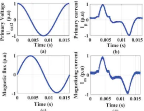
Using numerical trapezoidal integration [30] and (6), (8), (9), magnetic flux and magnetizing current can be computed by having measured primary voltage $3451(&) and current 7*<(&) of transformer. Fig. 10 (a) and (b) show one period of the steady state measurement of a voltage and current, respectively. Computed magnetic flux and magnetizing current are illustrated in Fig. 10 (c) and Fig. 10 (d), respectively. Note that computing 7.(&) needs the derivative of magnetic flux, then introduces high-pass filter, and finally, leads to an increase of high frequency noise.
Fig. 10. (a) Measured primary voltage of transformer ($3451), (b) Measured primary current of transformer (7*), (c) Calculated magnetic flux of transformer (G.) and (d) Calculated magnetizing current of transformer (7.)
Due to the nonlinear characteristics of sensor, there is less accuracy in low value of current. As the sensor is designed to measure inrush current and full load current, there exists an
TABLE IV
RELATIVEERROR OF JA PARAMETERSACHIEVED BY DIFFERENT START
POINTSCOMPARED TO INITIALJA PARAMETERS
Parameters Selection1 Selection2 Selection3 a 1.4% 0.051% 0.64% k 19% 0.1% 40% Y 1.7% 0.078% 0.6% c 25% 0.19% 45.5%
TABLE V
RELATIVEERROR OF JA PARAMETERSACHIEVED BY DIFFERENT START
POINTSCOMPARED TO JA PARAMETERSACHIEVED BY 20%OFPERIOD
Parameters Selection1 Selection2 Selection3 a 1.4% 0.0046% 0.68% k 19.48% 0.0114% 66.9% Y 1.5% 0.073% 0.63% c 33.7% 0.0615% 83.07%
TABLE VI
RELATIVEERROR OF HYSTERESISCYCLE AREA
Compared with Selection1 Selection2 Selection3 Initial Hysteresis cycle
area
1.9% 0.0029% 6.37% Hysteresis cycle area
obtained by 20% of period
1.9% 0.01% 6.3%
TABLE VII
TRANSFORMERELECTRICALPARAMETERS
Symbol Values '* lJll??<•–&—pm
+* lJ‡ˆ‡<—#–&—pm
error. This is due to the great difference between the maximum rating of the sensor and the maximum value of the measured primary current in steady state and no load condition.” Consequently, the current is deformed, and nonlinearities exists.
To estimate the hysteresis loop of desired transformer, it is required to compute the magnetic field and magnetic induction through previous variables (10), (13). The corresponding hysteresis loop is depicted in Fig. 11 (a). In order to perform an accurate identification process, the signal is filtered by a nonlinear median filter of even order n.
The filtered signal is shown in Fig.11 (b).
Fig. 11. (a) Computed hysteresis cycle using measurements (! " #), (b) Filtered hysteresis cycle.
A transient state appears on filtered hysteresis loop due to the numerical filtering. Therefore, we do not have a symmetric and complete hysteresis loop. Based on analysis done in section IV, a part of hysteresis cycle including coercive field and extremum of hysteresis loop is necessary for parameters identification. In our case study, two parts of hysteresis with correct characteristics which are not affected by nonlinearity of sensor is selected. These two parts represent about 40% of the whole hysteresis cycle with and without extremum point. All the procedure of identification is done as in section IV #3, #.4‘ H.4‘ >˜™xš
›œ " #.4‘. Table VIII shows the parameters of JA model obtained considering two different mentioned parts of hysteresis cycle.
Fig. 12 shows the comparison between experimental and simulated hysteresis cycles. Parameters in Table VIII are used in simulation. The simulation using the parameters obtained by part of hysteresis cycle with extremum point is in good agreement with experimental data, Fig.12.
Fig. 12. Comparison of experimental and simulated hysteresis cycles
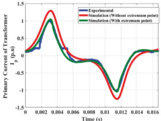
Fig. 12 confirm the conclusion of section IV that having the extremum point is necessary for an accurate identification process. To confirm the whole model proposed in sections II.C and III., the simulated primary current is also compared with the measured one on test bench, Fig.13.
Fig. 13. Comparison of simulation result and experimental measurement of primary current
Fig.13 demonstrates the accuracy of the method. The difference of current in low values is due to the impact of sensor.
VI. CONCLUSION
In this paper, train traction chain including nonlinear transformer is modelled using the bond graph method which allows us to consider physical phenomena including causalities. This method leads to simulation scheme based on state space equation to accurately simulate the behavior of the traction chain. The transformer model considers nonlinearity of magnetizing inductance using JA model. The JA model is rewritten to be avoid algebraic loop while state equations are solved.
Due to non-ideal test conditions, analyses are done considering entire and uncomplete hysteresis cycle. It is shown that JA parameter identification can be done with a part of the hysteresis cycle that includes the extremum point and coercive field. Then, the parameter identification is performed on a transformer included in a test bench representative of a railway traction chain. The simulated primary current is compared with the measured one and shown a great accuracy. This paper demonstrates that few measurements are needed to completely and precisely identify parameters of power transformer in order to simulate it. These simulations used during validation and
TABLE VIII IDENTIFIED JA PARAMETERS Symbol Values H/45 ??ˆl‡ˆ„‰JŠ c Š„J‡‡ a ?l†Jƒ Y lJlll†Š…‰Š \ lJ††„Š
verification process may lead to a clear evaluation of performances of the traction chain.
As the proposed methodology provides a minimal order state space system of equations, it has to be checked in future work that associated solving may be performed on real time simulator.
REFERENCES
[1] M. A. Rahman and A. Gangopadhayay, "Digital simulation of magnetizing inrush currents in three phase transformers," IEEE Trans. Power Del., Vols. PWRD-1, no. 4, p. 235–242, 1986.
[2] M. Elleuch and M. Poloujadoff, "New transformer model including joint air gaps and lamination anisotropy," IEEE Trans. Magn., vol. 2, no. 5, p. 3701– 3711, Sep. 1998.
[3] Z. Zhang, X. Yin, W. Cao, X. Yin, "The Mathematical Analysis and Modeling Simulation of Complex Sympathetic Inrush for Transformers," in
IEEE Conference, London, UK,, 2017.
[4] M.G. Say, Alternating Current Machines, 4 ed., Pitman Publishing Ltd. Acrobat 7 Pdf 18.5 Mb, 1976, pp. 142-146.
[5] NAIDU, S.R., "Simulation of the hysteresis phenomenon using Preisachs theory," IEE Proc. A, vol. 137, no. 2, pp. 73-79, 1990.
[6] J.G. Zhu, S.Y.R. Hui, V.S. Ramsden, "Discrete modeling of magnetic cores including hysteresis eddy current and anomalous losses," Proc. Inst. Elect. Eng., vol. 140, p. 317–322, 1993.
[7] Jiles, D.C.; Atherton, D.L., "Theory of ferromagnetic hysteresis," J. Magn. Magn. Mater., vol. 61, pp. 48-60, 1986.
[8] Faouzi Aboura, Omar Touhami, "Modeling and Analyzing Energetic Hysteresis Classical Model," in
International Conference on Electrical Sciences and Technologies in Maghreb (CISTEM), Algiers,
Algeria,, 2018.
[9] Xu Wei ; Fengbo Tao ; Jiansheng Li ; Chao Wei ; Xiaoping Yang ; Caibo Liao, "Modelling minor hysteresis loops and anisotropy with classical Jiles-Atherton model," in Chinese Automation Congress
(CAC), Jinan, China, 2017.
[10] V. Oiring de Castro Cezar, P. Lombard, A. Charnacé, O. Chadebec, L-L. Rouve, J-L. Coulomb, F-X. Zgainski and B. CaillaultS, "Numerical simulation of inrush currents in single-phase transformers using the Jiles-Atherton model and the finite element method," in IEEE Conference on Electromagnetic
Field Computation (CEFC), Miami, FL, USA, 2016.
[11] Lauri Perkkiö, Brijesh Upadhaya, Antti Hannukainen, Paavo Rasilo, "Stable Adaptive Method to Solve FEM Coupled With Jiles–Atherton Hysteresis Model," IEEE Transactions on Magnetics, vol. 54, 2017.
[12] O. Ozgonenel H. Dirik I. Guney O. Usta, "A New Transformer Hysteresis Model in MATLAB ™ Simulink," in IEEE Bucharest PowerTech, Bucharest, Romania, 2009.
[13] Jiles, D.C., Thoelke, J., Devine, M., "Numerical determination of hysteresis parameters for the modeling of magnetic properties using the theory of ferromagnetic hysteresis," IEEE Trans. Magn., vol. 28, no. 1, p. 27–35, 1992.
[14] Leandro dos Santos Coelho, Juliano Pierezan, Nelson Jhoe Batistela, Jean Vianei Leite, Sotirios K. Goudos, "Multiobjective lightining search applied to Jiles-Atherton hysteresis model parameter estimation," in 7th International Conference on Modern Circuits
and Systems Technologies (MOCAST), Thessaloniki,
Greece, 2018.
[15] M. Hamimid, M. Feliachi, S. Mimoune, "Modified Jiles–Atherton model and parameters identification using false position method," Physica B: Condens.
Matter, vol. 405, no. 8, p. 1947–1950, 2010.
[16] K. Chwastek, and J. Szczyglowski, "An Alternative Method to Estimate the Parameters of Jiles-Atherton Model," Journal of Magnetism and Magnetic
Materials, vol. 314, no. 1, pp. 47-51, 2007.
[17] Xiaohui, W., David, W.P.T., Mark, S., et al., "Numerical determination of Jiles-Atherton model parameters," COMPEL-Int. J. Comput. Math. Electr.
Electron. Eng., vol. 28, no. 2, p. 493–503, 2009.
[18] G. Abdulsalam, W. Xu, W.L.A. Neves, X. Liu,, "Estimation of Transformer Saturation Characteristics from Inrush Current Waveforms," IEEE Trans. Power
Deliv, vol. 21, p. 170–177, 2006.
[19] T.C. Monteiro, F.O. Martinz, L. Matakas, W. Komatsu, "Transformer Operation at Deep Saturation: Model and Parameter Determination," IEEE Trans.
Ind. Appl., vol. 48, p. 1054–1063, 2012.
[20] M. Elleuch and M. Poloujadoff, "A contribution to the modeling of three phase transformers using reluctances," IEEE Trans. Magn., vol. 32, no. 2, p. 335–343, Mar. 1996.
[21] Haitham Safar, "Power transmission line analysis using exact, nominal π, and modified π models," in The
2nd International Conference on Computer and Automation Engineering (ICCAE), Singapore, 2010.
[22] G. Gandanegara, X. Roboam, B. Sareni, G. Dauphin-Tanguy,, "Modeling and Multi-time Scale Analysis of Railway Traction Systems Using Bond Graphs," in Proceedings of International Conference
on Bond Graph Modeling and Simulation, 2001.
[23] D.C. Karnopp, R. Rosenberg, A.S. Perelson, "System dynamics: a unified approach," Transactions
on Systems, Man and Cybernetics, pp. 724-724, 1976.
[24] M. F.Jaafar, M. A. Jabri,, "Study and Modeling of Ferromagnetic Hysteresis," in International Conference on Electrical Engineering and Software Applications, Tunisia,, 2013.
[25] W. T. Conffey, Yu. P. Kalmyyov and J.Waldron, "The Langevin Equation with Applications in Physics, Chemistry and Electrical Engineering," 1996.
[26] Wang, X., Thomas, D.W.P., Sumner, M., et al., "Characteristics of Jiles–Atherton model parameters and their application to transformer inrush current simulation," IEEE Trans. Magn., vol. 44, no. 3, p. 340– 345, 2008.
[27] Aluffi-Pentini, F., Parisi, V. and Zirilli, F., "Global Optimization and Stochastic Differential Equations,"
Journal of Optimization Theory and Applications, vol.
47, no. 1, pp. 1-16, 1985.
[28] D. Zhang, Y. Liu, S. Huang, "Differential Evolution Based Parameter Identification of Static and Dynamic J-A Models and Its Application to Inrush Current Study in Power Converters," IEEE Trans. Magn., vol. 48, no. 11, pp. 3482-3485, 2012.
[29] Karaboǧa, D. & Okdem, Selcuk., " A simple and global optimization algorithm for engineering problems: Differential evolution algorithm," in Turkish
Journal of Electrical Engineering and Computer Sciences, 2004.
[30] K. Atkinson, W. Han, D. Stewart,, "Numerical Solution of ordinary differential equations," Wiley