an author's http://oatao.univ-toulouse.fr/20188
https://link.springer.com/article/10.1007/s40435-014-0105-6
Thabet, Hajer and Ayadi, Mounir and Rotella, Frédéric Towards an ultra-local model control of two-tank-system. (2016) International Journal of Dynamics and Control, 4 (1). 59-66. ISSN 2195-268X
Towards an ultra-local model control of two-tank-system
Hajer Thabet • Mounir Ayadi • Frédéric RotellaAbstract This paper deals with the design of an ultra- local model control. The proposed approach is based on the estimation of the ultra-local model parameters using least squares resolution technique instead of numerical derivation technique. The closed-loop control is implemented through an adaptive PI in order to reject the influences of the dis- turbance and noise output signais. Its main advantages are: its simplicity and its robustness with respect to the parame- ter uncertainties of system. In this paper, it is processed to test the efficiency of the parameter estimation method com- pared with the performance of numerical derivation tech- nique. The method is applied to the water level control of a two-tank-system. Numerical simulations show that the gen- erated desired trajectory is followed in an efficient way even with severe operating conditions.
Keywords Ultra-local model control • Least squares method • Robustness analysis • Adaptive PI controller • Two-tank-system
1 Introduction
Today, the complex systems control remains an open prob- lem. Their implemented solutions are often partial and of
significant complexity because of the need to find an accu- rate model of the system. In this case, instead of relying on a more accurate knowledge structure of the controlled system model, the ultra-local model control (called also free-model control) is based on a simple local modeling decorrelated from the physical reality. This approach, recently introduced by Fliess and Join [1- 3], is also based on the rapid estima- tion techniques [4]. lt does not estimate the unknown para- meters. Instead, it estimates a variable composed of error model (coming from the difference between the unknown real model and the simple used model) and disturbances.
This new control approach has many advantages. First it is easy to implement, it is also highly robust. Moreover, the time of implementation is reduced thanks to the low parameter number of design. The advantages of ultra-local mode] con- trol and of the corresponding adaptive PID controllers led to a number of exciting applications in various fields [1, 4- 14].
For example, in [1], numerical derivation (ND) techniques have been employed to estimate noisy signais. This estima- tor can be easily implemented in the form of discrete-time linear filter to mitigate the measurements noises. However, the estimation of a single variable by the numerical deriva- tion technique is insufficient to obtain the desired perfor- mance, particularly, if the estimation of the second parameter is required. For this reason and in order to improve these per- H. Thabet (C8J) · M. Ayadi
Laboratoire de Recherche en Automatique, Ecole Nationale d' ingé nieu rs de Tunis, Université de Tunis El Manar, 1002 Tunis, Tunisia
e-mail : [email protected] M.Ayadi
e-mail : [email protected] F.Rotella
Laboratoire de Génie de Production , Ecole Nationale d'ingénieurs de Tarbes, 65016 Tarbes Cedex, France
e-mail: [email protected]
formances, we propose in this paper a new ultra-local model control approach based on the linear least squares (LS) tech- nique to estimate the ultra-local model variables.
The comparison between the numerical derivation tech- nique and the linear least squares method estimating the ultra-local model parameters, is kept here to clarify the per- formance improvement and effectiveness of proposed con- troller design.
The present work deals with the automatic water level con- trol in the flow channels which was developed by an abundant
=
ay
(v) _ ( • ( v - 1) ( v+ l) (y) ·
(K
)
)
literature (see [10, 15- 17]). The water level control consti- tutes a desired trajectory tracking problem with rejection of flow disturbances with nonlinear dynamics. In this paper, theultra-local model control is applied to two-tank water system which is considered as a nonlinear system of first-order.
The paper is organised as follows: the concept of ultra-
local model control is presented in the second section. Two different methods of parameter estimation (the least squares and the numerical derivation methods) are elaborated in Sect. 3. The two-tank-sy stem model, the control design and the simulation results are given in the Sect. 4. Finally, some concluding remarks are presented in the Sect. 5.
2 Ultra-local model control 2.1 Basic idea
2.2 Adaptive PI controller
If v
=
1 in (3), the desired closed-loop behavior is obtained thanks to an adaptive PI or, in abbreviated, a-PI [1]. The control signal is given by:-F (t)
+
yd
(t)+
Kpe (t)+
Ktf
e (t)u(t) (4)
a (t)
where
- yd (t) is the desired output trajectory, obtained by flat- ness properties [18- 20) that is well adapted to solve the trajectory planning problems,
- e (t)
=
yd (t) - y (t) is the tracking error.-K p, Kt are suitable gains, the tuning of which is quite straightforward.
The ultra-local model control is based on local modeling,
constantly updated, from the solely knowledge of input-
Remark 2 The nonlinear system
.x
tially fiat if we can find fiat outputs:f (x, u) is differen-
output behavior. For the unknown differential equation:
Z -- h f ( X , U., U , .•. , U(pl) (5)
E ( y,y•, ... , y (l) , u ,, u , ... , u
(K))
-
- 0 (1) such that:X
-
- <p/
.
Z, Z,.
Z.
, · · · , Z(r)
)
which can be linear or not, where u is the system input, y isthe system output and E is a sufficiently smooth fonction of
u
_-
,-1,z,z
•,z
••,
...,z
(r +l))(6)
its arguments, we assume that for an integer v , 0 < v < L,-
B
(
E
-)
-1-
0, the implicit fonction theorem then allows to writeV
the following equation:
z is called the fiat output which can be or not the system output. As represented above in the Eq. (6), the states and the input variables of the system are expressed in terms of the fiat outputs and their higher derivatives.
y - <p t , y,y, . . . ' y 'y ' ... ' y 'u, u , ... 'u
(2)
The a-PI controller of the Eq. (4) compensates the unknown term F (t) and a (t).approximatively describing the input-output behavior. Ultra-
local model control consists in trying to estimate via the input and the output measurements what can be compensated by control in order to achieve a good output trajectory tracking. This implies the construction of a purely numerical model also called ultra-local model of the system that can be written as:
Remark 3 If v
=
1, we brought back with (4) to a pure integrator stabilization. Therefore, the two gains setting K pand Kt become very simple in contrast to classical PI (see
[21) for more details).
Combining Eqs. (3) and (4) yields to the fonctional equation
0:
yM (t)
=
F (t)+
a (t) u (t) (3)8 (e)
=
ë (t)+
Kpë (t)+
Kte (t)=
0(7)
The two quantities F (t) and a (t) contain the whole struc-
which the roots should be stable and a good tracking is asym- totically ensured, i.e.
tural information which should be identified in real time. Remark 1 The order of derivation v of y in (3) is strictly less
lim e (t)
= 0
t---->+ oo (8)
in general than y in (1), when this latter is known [1].
In many works, Fliess and Join indicate that in practice it is appropriate to consider an ultra-local model (3) in the cases of v = 1 or v = 2.
We obtain then a linear differential equation with constant coefficients of order 2. The tuning of Kp and Kt becomes therefore straightforward for obtaining a good tracking of yd. This is a major benefit when compared to the tuning of classic Pis.
3 Ultra-local model identification methods the following to solve the problem of the both estimation of F (t) and œ (t).
3.1 Numerical derivation (ND) method
In several works as [1, 2], a fast identification technique,
based on the numerical differentiations, is applied to estimate
the time-varying fonction F (t) thanks to the knowledge of
u(t) and y (t). Numerical derivation, which is a classic field of investigation in engineering and in applied mathematics,
is a key ingredient for implementing the feedback loop (3).
This solution has already played an important role in model-
based nonlinear contrai and in signal processing (see [4] for
further details and related references).
Important theoretical developments, which are of utmost importance for the computer implementation, may be found in [12].
The estimate of the first order derivative of a noisy signal
y is defined as follows (see [22]):
3.2 Least squares (LS) method
The estimation of the two parameters
ft
(t) and â (t) leads to the following principle of ultra-local model control:jd (t) -
F
(t)+
RP(
,
p- 1 ) (yd (t) - y(t))
u (t)
=
_
,
(13)a (t)
where R
(p,
p-
1 ) is a polynomial matrix with the operatorsof derivation p and integration p- 1 . In the case of adaptive
PI, the polynomial R is written as follows:
(14)
T
y
= -
T310
(T - 2t) y (t) dt
(9)
In the present approach, the application of control inputrequires the knowledge of the system output y and the desired
where [O, T], T > 0, is a quite short time window. This window is sliding in order to get this estimate at each time instant. Denoising of y leads to the following estimate:
T
trajectory yd, as well as the real-time estimation of the two
quantities F and œ in (3).
Assuming the numerical control with constant sampling period Te which allows to dispose on the system of constant control Uk - 1 between the instants (k - 1) Te and kTe and
y=
T2'1·
(2T-3t)y(t)dt0
(10) available information until the instant kTe, unless Uk.
The main aim of using a reduced ultra-local model
(i.e. choosing an order of derivation v
=
1 or v=
In these works [1], the quantity F (t) in (3) is updated at eachsampling time from the measurement of the output and the
knowledge of the input. At sampling time k (i.e. t
=
kTe,where Te denotes the sampling period), the estimation of F is written as:
A=
Yk - œu k - 1 (11)2) lies actually in the increasing of accuracy. In fact,
the reduction of the order of derivation v involves a lit-
tle sampling time Te of numerical control so a minimal
time of calculation. This increases accuracy and minimizes uncertainties.
From the simple model
y
(t)=
F (t)+
œ (t) u (t), the integration between two sampling instants gives:J
J
where Yk is the estimation of first derivation of the output
that can be laid at time k, œ is a non-physical constant design
parameter, and U k - l is the control input that has be applied to
the system during the previous sampling period. Based on the estimation of F, the control is calculated on (3) as follows:
-ft
(t)+
yd
(t)+
Kpe (t)+
Kr Je (t) k k Yk=
Yk-1+
F (t) dt+ a (t) u (t) dt k-1 k-1 (15) u (t)=
,
awhere a is chosen by the practitioner.
(12)
The identification of the two parameters F (t) and a (t)
is a difficult task via the algebraic derivation technique, par- ticularly, if the estimation of the second parameter a (t) is required. For this reason and in order to improve the perfor- mances, a new parameter estimation method is proposed in
Let frk and âk the mean values, in [(k - 1) Te , kTe ], of F (t)
and œ (t), finally we get:
(16)
J
)
=
-v
-v
Considering the following notations:yT _ Yk- Yk - 1
k - Te ,
H_T [ 1 ] (17)
k - U k- 1 ,
the previous relation (16) can be written in the following
form:
(18)
Since the regression matrix Hk
= [
1 Uk - 1 ] has a defaultrank then, this system is always consistent (i.e., rank [Hk]
=
rank [ Hk Yk ]). The aim is to seek at each instant kTe to
esti-mate 0k. According to the linear system resolution technique
detailed in [23], the general expression of estimation is:
(19)
where:
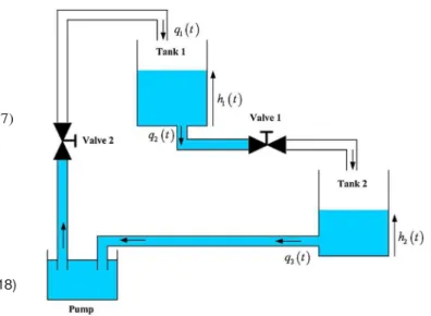
Fig. 1 Two-tank-system
of the lower tank. In the steady state, the conservation of the
total volume of water leads to q1 (t)
=
q3 (t).The nonlinear model of the considered system is as fol- lows:
sh1 (t)
=
q1 (t) - q2 (t)- Ht)
denotes the Moore-Penrose generalized inverse ofHk, that is mean the matrix X such as AXA= A [24],
- Âk is an arbitrary matrix of size (m x 1).
sh2 (t)
=
q2 (t) - q3 (t)with q2 (t)
=
k1/hi(i)
and q3 (t)=
k2Jh2 (t).(20)
The coefficients of matrix Âk appear as degrees of freedom that can be used to satisfy other relating constraints to the system control. However, these degrees of freedom are equal to the rank of lm+! - H11 Hk.
Based on the numerical knowledge of F and a, the
con-The term
k;/h:(i),
i=
1, 2, cornes from the turbulent regime of the water evacuation by the valves. The two para- meters k I and k2 represent the coefficients of the canalizationrestriction.
We obtain then the following model:
trol input is calculated in (3) as a closed-loop tracking of a · (t)
=
--v
k1 r,:---;-:::+
1 (t)h1
reference trajectory t --+ yd (t), and a simple cancellation of I
s
h1 (t) -
s
q1(21)
the nonlinear terms F and a.
The application ofthis new approach of ultra-local model control is considered in the case of a two-tank-system pre- sented in the following section.
4 Case study: two-tank-system 4.1 Model description
Consider the two-tank-system described in the Fig. 1 which
is constituted by two identical water tanks that have the same section S. Denote by h 1 (t) the water level in the upper tank,
which also represents the system output, h2 (t) the water level
in the lower tank, q1 (t) the input flow of the upper tank, q2 (t)
the output flow of the upper tank and q3 (t) the output flow
· k I r,:---;-::; k2 r,:---;-:::
h2 (t)
s
h1 (t) -s
h2 (t)These two equations are nonlinear due to the presence of the
term
/h(i),
hence the most difficult task in the control ofthis considered system will be the control of the water level
h1 (t) in different operating conditions.
4.2 Control design
In this work, we choose to generate a desired trajectory,
hf
(t)of system output, satisfying the constraints of the two-tank- system. Moreover, the trajectory generally satisfies the con- straints in terms of response time and rise time. Our reference trajectory ensures a transition between the initial water level
hf
(to)=
2 cm and the final water levelhf
(tf)
=
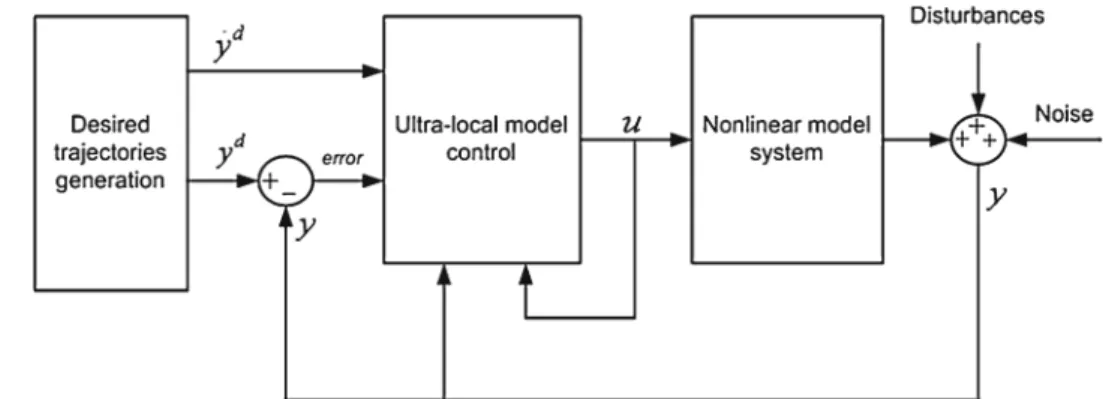
10 cm.Fig. 2 General struct ure of an
ult ra-lo c al mode! control
In the numerical simulations, taking the two transition
instants to
=
50 s and t f=
l 50 s, and calculating a fifthorder polynomial as reference trajectory between these two
instants . This trajectory satisfies the differentiability and con-
tinuity conditions at the in stants of set-point change.
The principle of an ultra-local model control of the non- linear considered system is summarised in Fig. 2 which rep-
resents the block diagram of the two-tank-system control in
closed-loop. The numerical values of two-tank-system para-
meters are given in the Table 1. The desired trajectories are
generated based on the concept of flatness [19,20]. We note
that the adding of noises and dis tur bances output aims to test
the robustness of the a-PI controller.
For comparison purpose, we have firstly implemented a
classical PI control. The controller parameters have been
manually tuned and are given in the Table 2. So, the tuning of
the classical PI gains has been done in two steps: Firstly, tun-
ing of the proportional gain on the un disturbed process. Sec-
ondly, tuning of the integral gain in order to achieve a good
perturbation rejection. Then, we have also implemented an
adaptive PI control using numerical derivation method. After
a few attempts, we set T
=
25Te in Eq. (9). The two para-meter K p and K I of a-PI controller, given in the Table 2,
are chosen according to a classical second order dynamics
Table 1 Parameter value s
( p2
+
K pp+
K1
=
0). For our control approach, the twogains Kp and K 1of adaptive Pl are chosen (see Table 2) in
order to stabilize the tracking error. The tuning of a-PI gains
is trivial by applied the functional equation (7).
4.3 Numerical simulations
The simulation results are summ arized in the following fig-
ures where we have studied the ultra-local mode! control with
two-tank-system in the presence of disturbances and noise s.
A centred white noise (normal law N(0,0.001)) is added to
the system output, prese nted in the Fig. 3, in order to test the
robustness of numerical simu lations of this work. At t
=
180s, a level water disturbance of 0.8 cm, which is due to a prob-
lem in the sensor, is applied to the system.
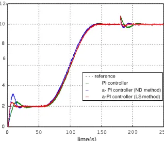
When the system is controlled by a classical PI controller,
we observe in Fig. 4 that the system output reaches the desired
trajectory in approximately 40 s with 0.5 cm overshoot. How-
eve r, a 12.75 s response time with 0.42 cm overshoot is
obtained when the system is controlled with our a-PI con-
troller. The parameters in this case are estimated using le ast
squares resolution method. It is then clear that the new control
strategy is better than the classic al PL 0.15 Parameter Value 0.1 Te 0 . 1 s 0 .05
s
332.5 cm 2 k1 42.1 cm512/s 0 k2 42.1 cm512/sTable 2 Controller parameters
-0.05
- 0.1
0 50 100 150
time (s)
200 250
Fig. 3 Centered white no ise of the output r
Gain Classical PI Adaptive PI (ND method) Adaptive PI
(LS meth od)
Kp 3 5 x l0- 1 10
Kt 9 x 10- 1 6 X 10- 2 3
- - - reference -- Pl controller -- a- Pl controller (ND method) -- a-Pl controller (LS method) 20 r 10 0 10 12r (a)Pl controller 10 10 [ 5 0 0 8 6
::
50 100 150 200 250(b)a-Pl controller (ND method)
4
0 50 100 150 200 250
2 (c)a-Pl controller (LS method)
0 0 50 100 150 lime(s) 200 250 20 l 10 0 0 50 100 lime(s) 150 200 250
Fig. 4 Reference and noisy system outputs in the case of the three different methods
(a) Pl controller
V--2
Fig. 6 Control inputs in the case of the three different methods (a)a-Pl controller (LS method)
0 50 100 150 200 250
(b)a-Pl cont ro lle r (ND method)
r---2
0 50 100 150 200 250
(c)a-Pl controller (LS method)
-20 L 0 50 100 150 200 250 2 0 -2 0 50 100 150 200 250 lime (s)
Fig. 5 Tracking errors in the case of the three different methods
In the Fig. 4, the a-PI control using least squares resolu-
tion has ensured better tracking of desired trajectory despite the addition of centered white noise to response system (see tracking errors given in Fig. 5). However, the tracking perfor-
mances are unsatisfactory for the a-PI control using numeri- cal derivation technique (Fig. 6). The response time (17.5 s) and the overshoot (1.1 cm) of the latter technique are greater in comparison with those of our proposed technique. We can observe in Fig. 4 that the consequence of level water distur- bance is smaller and rejected faster by the LS method than the numerical derivation method. A better robustness of the new control strategy with respect to external disturbances is then given thanks to the adaptive PI and the both on-line parameter estimation (see Figs. 4, 5, 6, 7).
lime (s)
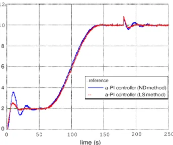
Fig. 7 Parameter estimation in the case of LS and ND methods To properly compare the robustness performances of the two adaptive controllers, we have tested the system dynam- ics in the case of parameter uncertainties. In the numerical simulations, we have treated the uncertainty of parameter S which is equal to 550 cm2 if 30 s < t < 170 s instead of 332.5 cm2. lt is clear that the tracking of desired trajectory is better when the ultra-local model parameters are estimated by LS method (see Fig. 9). In the Fig. 8, we can see that the proposed method is able to reject perturbations faster than the numerical derivation technique. Due to the parameter uncer
-tainties, we can observe that the control input of ND method achieved negative values (see Fig. 10
12r 10 8 30 r 20 10 0 10 L
(a)a-Pl controller (ND method)
6 0 50 100 150 200 250
(b)a-Pl controller (LS method)
4 3 2 2 0 0 50 100 150 lime (s) 1 200 250 0 50 100 150 lime (s) 200 250
Fig. 8 Reference and noisy system outputs in the case of LS and ND
methods-parameter uncertainties 50 % of S
(a)a-Pl controller (ND method)
0 50 100 150 200 250
(b)a-Pl controller (LS method)
2
0
-2L
Fig. 10 Control inputs in the case ofLS and ND methods-parameter
uncertainties 50 % of S
approach of parameter estimation, compared to the numerical
derivation method proposed in [1].
The main advantages of the proposed control method which is appreciable for industrial applications are as fol-
lows:
Allowing to bypass the difficult task of mathematical modeling and therefore complex identification proce- dures,
Leading to a straightforward gain tuning and a time
reduction of commissioning tests,
Providing a good robustness towards external dist ur-
bances and parameter variations of process.
0 50 100 150
lime (s)
200 250
Due toits properties of robustness, adaptability and simplic-
ity, the ultra-local mode] control provides outstanding
perfor-Fig. 9 Tracking errors in the case ofLS and ND method s- parameter
uncertainties 50 % of S
is more sensitive to parameter uncertainties, than the new estimation method presented in this paper. The both parame- ter estimation plays a very important role in the robustness of the proposed ultra-local model control with respect toper- turbation rejection and parameter uncertainties.
5 Conclusions
The contribution of the paper has allowed the design of a new water level controller, which is able to insure good trajectory
tracking performance even in severe operating conditions. An
improvement of performance is obtained with the proposed
mance with a very short time of implementation.92671474.
References
1. Fliess M, Join C (2008) Commande sans modèle et commande à
modèle restreint. e-STA 5:1-23
2. Fliess M, Join C (2013) Model-free control. Int J Control 810345.
doi:10.1080/00207179
3. Fliess M, Join C, Riachy S (2011) Rien de plus utile qu'une bonne
théorie : la commande sans modèle, 4èmes Journées Doctorales
/Journées Nationale s MACS, JDJN-MACS'201 l, Marseille
4. Fliess M , Join C (2008) Non-linear estimation is easy. Int J Mode!
ldentif Control 4:12-27
5. Abouaïssa H, Fliess M, Iordanova V, Join C (2011) Prolégomènes
à une régulation sans modèle du trafic autoroutier. Conférence
Méditerranéenne sur !'Ingénierie sûre des Systèmes Complexes,
Agadir 2 c 0 -2 L 0 r 0 0 0 L - - - reference a-Pl controller (ND meth od)--- a-Pl controller (LS method)
6. Fliess M, Join C, Mboup M (2010) Algebraic change-point detec- tion, applicable algebra in engineering. Commun Comput 21:131-143
7. Fliess M, Join C, Perruquetti W (2008) Real-time estimation for switched linear systems. ln: 47th IEEE conference on decision and contrai, Cancun, pp 409-414
8. Fliess M, Join C, Riachy S (2011) Revisiting some practical issues in the implementation of model-free control. In: 18th IFAC world congress , Milan
9. Join C, Masse J, Fliess M (2008) Etude préliminaire d' une com- mande sans modèle pour papillon de moteur , a model-free contrai for an engine throttle: a preliminary study. Journal européen des systèmes automatisés 42:337-354
10. Join C, Robert G, Fliess M (2010) Model-free based water level contrai for hydroelectric power plants. ln: IFAC conference on contrai methodologies and tecnologies for energy efficien cy,
CMTEE'2010, Vilamoura
11. Mboup M, Join C, Fliess M (2007) A revised look at numerical differentiation with an application to nonlinear feedback control. In: Proceedings of the 15th mediterranean conference on contrai and automation, MED' 2007, Athnes
12. Mboup M , Join C, Fliess M (2009) Numerical differentiation with annihilators in noisy environment. Numer Algorithm 50:439-4 67 13. Michel L, Join C, Fliess M, Sicard P, Chériti A (2010) Model-free
contrai of DC/DC converters. In: 12th IEEE workshop on contrai and modeling for power electronics, COMPEC2010, Boulder 14. Rezk S, Join C, El Asmi S (2012) lnter-beat (R-R) intervals analysis
using a new time delay estimation technique. In: 20th European signal processing conference , EUSIPCO'2012, Bucarest
15. Litrico X, Fromion V (2009) Modeling and contrai of hydrosys- tems. Springer, London
16. Zhuan X, Xia X (2007) Models and contrai methodologies in open water flow dynamics: a survey. IEEE Africon, Windhoek 17. Join C, Robert G, Fliess M (2010) Vers une commande sans mod-
èle pour aménagements hydroélectriques en cascade, 6ème Con- férence Internationale Francophone d' Automatique , CIFA'2010, Nancy
18. Ayadi M, Haggège J, Bouallègue S, Benrejeb M (2008) A digital flatness-based contrai system of a DC motor. Stud Inform Control SIC 17:201-214
19. Fliess M, Lévine J, Martin P, Rouchon P (1995) Flatness and defect of non-linear systems: introductory theory and examples. Int J Con- trol 61:1327-1361
20. Rotella F, Zambettakis I (2007) Commande des systèmes par plat- itude, Éditions Techniques de l' ingénieur , S7450
21. Astréim KJ, Hagglund T (2006) Advanced PID controllers, 2nd edn. Instrument Society of America, Research Triangle Park 22. Garda Collado FA, d' Andria-Novel B, Fliess M , Mounier H (2009)
Analyse fréquentielle des dérivateurs algébriques. XXIIe Coll, GRETSI, Dijon
23. Rotella F, Borne P (1995) Théorie et pratique du calcul matriciel. Éditions Technip, Paris
24. Ben-Israel A, Greville TNE (1974) Generalized inverses: theory and applications . Wiley, New York