Explaining single predictions : a faster method

Official URL

https://doi.org/10.1007/978-3-030-38919-2_26

Any correspondence concerning this service should be sent

to the repository administrator:

[email protected]

This is an author’s version published in:

http://oatao.univ-toulouse.fr/26286

Open Archive Toulouse Archive Ouverte

OATAO is an open access repository that collects the work of Toulouse

researchers and makes it freely available over the web where possible

To cite this version: Ferrettini, Gabriel and Aligon, Julien and

Soulé-Dupuy, Chantal Explaining single predictions : a faster

method. (2020) In: International Conference on Current Trends in

Theory and Practice of Computer Science (SOFSEM 2020), 20

January 2020 - 24 January 2020 (Cyprus).

Explaining single predictions : a faster method

Universit´e de Toulouse, UT1, IRIT, (CNRS/UMR 5505) [email protected]

Abstract. Machine learning has proven increasingly essential in many fields. Yet, a lot obstacles still hinder its use by non-experts. The lack of trust in the results obtained is foremost among them, and has inspired several explanatory approaches in the literature. In this paper, we are investigating the domain of single prediction explanation. This is per-formed by providing the user a detailed explanation of the attribute’s influence on each single predicted instance, related to a particular ma-chine learning model. A lot of possible explanation methods have been developed recently. Although, these approaches often require an impor-tant computation time in order to be efficient. That is why we are inves-tigating about new proposals of explanation methods, aiming to increase time performances, for a small loss in accuracy.

Keywords: Machine learning · Explanation model · predictive model

1

Introduction

Many explanation methods exist in the literature, to overcome the ”black box” problem of model prediction results. These methods are mainly devoted to ex-plain a predictive model in a global way. These methods are not relevant when a domain expert user (for instance a biologist) has to study the behavior of particular dataset instances over a predictive model (for instance in the con-text of cohort study). In this direction, previous studies offer the possibility of explaining single instance prediction, over a model, as in [12] and [2]. One ma-jor problem of these contributions is the complexity of the proposed algorithms (O(n2_{)). Thus, it is illusory for domain experts wishing to apply this method}

to study the behavior of a set of instances. This complexity makes them very slow to calculate on datasets with a large number of attributes. Our work fits the general ambition to help a domain expert user to (re)find motivation to get involved in data analysis operations. In particular, our goal is to rely as much as possible on her/his area of expertise, while limiting knowledge in data analysis. In this paper, we aim to facilitate the use of predictive models by explaining their predictions in a way balancing information and computing time.

The contributions presented in this paper include:

– A comparison between two selected prediction explanation approaches. This is done to decide which method to use as a basis, among the two closest to our scope.

– Two new methods for classification explanations, based on [12], and adapted to achieve a better calculation time, without losing too much information. The paper is organized as follows. Section 2 explores some work already done in the domain of prediction explanation. In particular, the literature helps us to identify an explanation method as close as possible to our scope: helping non expert users to understand the inner workings of a predictive model. Then, in Section 3, we propose improvements of the selected method to achieve a better calculation time, without losing too much information. Finally, we experiment our proposals to check their interest in terms of computation time and their impacts in terms of loss of accuracy.

2

Related works

Explaining the influence of each attribute (of a dataset) on the output of a predictive model have been explored largely. An example of the works pertain-ing to global attribute importance on a model can be seen here: [1]. The most recent methods are based on swapping the values of attributes in the dataset and analysing which swap affect the trained model predictions the most. The more modifying the attributes values affects the predictions, the most this at-tribute is considered important for the model, as a whole. These methods are often used during feature selection, allowing to opt out attributes not used by the model. Many ways of explaining single predictions have been explored but these methods often struggle between being too simplistic, or too complex to be interpreted by a human, notwithstanding the problem of computation time, which can become problematic for more advanced methods. The possible appli-cations of prediction explanations have been investigated by [8]. According to their paper, the interest for explaining a predictive model is threefold:

– First, it can be seen as a mean to understand how a model works in general, by peering at how it behaves in diverse points of the instance space. – Second, it can help a non expert user to judge of the quality of a

predic-tion and even pinpoint the cause of flaws in its classificapredic-tion. Correcting them would then lead the user to perform some intuitive feature engineering operations.

– Third, it can allow the user to decide the type of model preferable to another one, even if he has no knowledge of the principles underlying each of them. A great number of works pertaining to prediction explanation led to [6], which theorized a category of explanation methods, named additive methods, and pro-duced an interesting review of the different methods developed in this category. Some of these methods are described in detail in [3] and [10]. They are sum-marized in [6] as methods attributing for a given prediction, a weight to each attribute of the dataset. This creates a very simple ”predictive model”, mimick-ing the original model’s behavior locally. Thus, we have a simple interpretable linear model which gives information on the original model’s inner working in a

small vicinity of the predicted instance. The methods from which these weights are attributed to each attributes varies between the different additive methods, but the end result is always this vector of weights. This article has highlighted several interesting properties about these methods, which make it a very useful theoretical object : Local precision: The system describes precisely the model in the close vicinity of the explained instance. ”Missingness”: If an attribute is missing for the prediction, the method does not give it a weight, or gives it a weight of zero. Consistence: If the explained model changes in a way that makes an attribute more important, or does not change its importance, its attributed weight is not diminished. This property is important, as some of the early pre-diction explanation methods could have an erratic behavior in some cases, as shown in an example of [6]. Other lines of reasoning have been explored, as in [2], which explored prediction explanation in the point of view of model perfor-mance. Meaning that their metric shows which feature improves the performance of the model, rather than which feature the model consider as important for its prediction. If this line of reasoning is really interesting for the model explanation field, it does not correspond to our scope as well as other methods, as we are aiming to help users understand how a model works, and not how to improve it. In this paper, we are aiming to facilitate the understanding of any machine learning models for user without particular knowledge on data analysis or ma-chine learning. Thus, it is more relevant to focus on the works as [12] or [3], cited as additive methods, as they generate a simple set of importance weights for each attribute. This set of weights is easy to interpret, even for someone with-out expertise on machine learning. Yet, these methods have a major deterrent: their computation time makes them difficult to use for the average user. That is why [6] explored methods to generate explanations faster, but at the cost of very restricting hypotheses, as the Independence of each attributes of the dataset, or the linearity of the model, which is not always the case. Thus, we are aiming for a simplification to reduce computational time of methods like [12], but ap-plicable in a more generic way than [6]. With this work, we want to facilitate the generation of prediction explanation, without having to restrict ourselves to a given set of models. The ability to explain the prediction of any model thus appears to be a key point for allowing a broader public (non expert) to access and use machine learning models. This need led us to consider the diverse ex-planation systems, developed in the literature, as having a major interest for giving more autonomy to domain experts performing data analysis tasks. Yet, the computational load found in the most generic methods can be a hindrance to their use. In this paper, we seek to select a prediction explanation method as generic as possible and try lowering its computing time without loosing too much information.

3

Choosing a basic explanation method

In order to start developing a faster additive explanation method, we have to select an algorithm from the literature and reduce its complexity without losing

too much information. For this, we compare two methods developed by the authors of [11] and [12], as they are classical and similar in their design, but different in their interpretation.

3.1 Prediction explanation methods

Given a dataset D of instances and a set of n attributes A = {a1, .., an}, each

attribute being either continuous or nominal, its possible values are then integers or real number. Each instance x ∈ D is defined by the values of each of its attributes : x = {x1, ..., xn}, ∀i ∈ 1..n, xi ∈ N ∨ xi ∈ R. We want to explain

a predictive model, based on the function f : D → [0, 1], whose result is the confidence score in the classification of the instance x for a class C, as predicted by the model.

Information loss method One of the first definition for classification explana-tion is proposed in [11]. According to their method, the influence of an attribute ai on the classification of a given instance is defined as the difference between

the classifier prediction (with ai) and its prediction without the knowledge of

attribute ai. Thus, given a dataset of instances described along the attributes of

A, the influence of the attribute ai on the classification of an instance x by the

classifier confidence function f on the class C can be represented as:

inf_f,aC _{i(x) = f (x) − f(x\a}i) (1)

Where f (x\ai) represents the probability distributions for a classification of the

instance x by the classifier f without knowledge of the attribute ai. We name

this method as the information loss method (shortened as loss method ). Information gain method In more recent works, as in [12], another possible formula is based on the information brought by an attribute in the dataset:

inf_f,aC i(x) = f (xai) − f(∅) (2) Where f (xai) represents the probability that the instance x is included in the

class C with only the knowledge of the attribute ai(according to the predictive

model). We name this method as the information gain method (shortened as gain method). In order to simulate the absence of an attribute, the authors of [11] theorize possible approaches, among which we selected to retrain the classifier without the corresponding attribute.

Comparing the two methods : Toy example on a basic dataset As an illustration, and in order to ease interpretations, we apply these two methods in a simple ID3 decision tree [7], trained on the well-known Fisher’s Iris dataset1_.

1

As a decision tree is a naturally interpretable model, and Iris dataset is well studied in the literature, it is easy to compare and interpret the two methods and detect eventual problems. We use Weka [4] and OpenML [13] to perform the data management and model training while ensuring the reproductibility of all experiments. OpenML is a machine learning collective platform. It includes a repository of datasets and workflows, in which each user can upload any new dataset and run any data mining task on them. To estimate the reliability of loss and gain methods, we apply a 5-fold cross validation on the Iris dataset. The explanations of both methods are generated on the validation set, for each itera-tion of the cross-validaitera-tion. We generate thus predicitera-tion explanaitera-tions of Weka’s J48 tree classifier, for the whole Iris dataset. Then, we compare those explana-tions to the decision tree, and get a general sense of the explanation accuracy. Each instance of the Iris dataset is composed of four attributes: petal length, petal width, sepal length and sepal width. Each instance is included in one of these three classes: Iris Setosa, V ersicolor or V irginica.

Fig. 1: Repartition of the 3 different classes by petal length and width, with their corresponding generalization according to the decision tree

Fig. 2: A decision tree trained on Iris

By a simple look at the trained decision tree Figure 2, we see the influence of the loss method should be zero for the sepal length and width attributes, as they are not used by the tree at all. Moreover, the Setosa class instances should only be influenced by petal width, as it is the only attribute used to classify them. For Iris Virginica and Versicolor, we can expect a high influence from petal width, and a lower from petal length influence, yet still significant as these two attributes are used. We can now compare these expectations to the

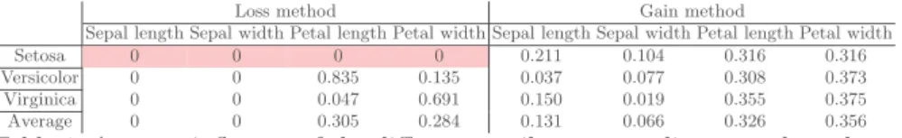
Loss method Gain method

Sepal length Sepal width Petal length Petal width Sepal length Sepal width Petal length Petal width

Setosa 0 0 0 0 0.211 0.104 0.316 0.316

Versicolor 0 0 0.835 0.135 0.037 0.077 0.308 0.373

Virginica 0 0 0.047 0.691 0.150 0.019 0.355 0.375

Average 0 0 0.305 0.284 0.131 0.066 0.326 0.356

Table 1: Average influence of the different attributes according to each explana-tion method, for each class of instances

results indicated Table 1. We see the loss method does not behave as expected for the Setosa instances, as all the attributes are being given an influence equals to 0. This can be understood by looking at the representation of the concept learned by the tree Figure 1. We note that, by removing one of the attributes between petal length and petal width, it remains possible to separate the Setosa class linearly from the others using only the petal length, and still maintain a 100% confidence in the classification. Thus, each attribute is considered as incon-sequential by the loss method, when classifying Setosa instances. This implies that, for every dataset in which two attributes carry very similar information, the loss method will be unable to generate a satisfying explanation.

The gain method, on the other hand, gives an importance to all the four at-tributes about Setosa instances. A minimal importance is given for sepal length and width, unlike the petal length and width. It is easily understandable by observing the graphs of repartition of the different classes (Figure 1). We note the petal length and width can easily separate the three classes, but the sepal attributes are less defined in their separation. This is especially true for the V ersicolor class, as it is mixed with its two adjacent classes. Thus, the gain methodseems to be closer to what the decision tree is doing when being trained. Finally, we conclude the main difference of the two methods relies in the fact they are not trying to calculate the same thing: the loss method is based on the information lost by the model when removing an attribute, while the gain method is based on the information brought by each attribute. Yet, we remark the loss method has an aberrant behavior when confronted with two attributes bringing the same information. Thus, the gain method seems the best proposal for a pre-diction explanation. But this method has its flaws: it only takes into account the information brought by each attribute, independently. In many datasets, the at-tributes are often interdependent. Our next objective is to consider the influence of group of attributes as described in the next section.

4

Toward a more efficient method

In order to answer the problems of interaction between attributes, we propose to take inspiration from the work of [12]. We are here in a framework close to the situation of a game called ”coalitions”, where each group of attributes can have an influence on the prediction of the model. Therefore, we cannot consider each attribute as independent, but all the possible combinations of attributes.

The influence of an attribute is measured according to its importance in each coalition. We can then refer to the coalition games as defined by Shapley in [9]: A coalitional game of N players is defined as a function mapping subsets of players to gains g : 2N

7→ R. The parallel can easily be drawn with our situation, where we wish to assess the influence of a given attribute in every possible coalition of attributes. We then look at not only the influence of the attribute, but also its use in all subsets of attributes. We thus define the complete influence of an attribute ai∈ A on the classification of an instance x (the notations remain the

same as in 3.1): IC

ai(x) =

X

A′⊆A\ai

p(A′, A_{) ∗ (inff,(A}C ′∪ai)(x) − inf

C

f,A′(x)) (3) With p(A′_{, A) a penalty function accounting for the size of the subset A}′_.

Indeed, if an attribute changes a lot the result of a classifier, depending of a lot of attributes, it can be considered as very influential compared to the others. On the opposite, an attribute changing the result of a classifier, whereas this classifier is based on a few number of attributes, cannot be considered to have a decisive influence. The Shapley value [9] is a promising candidate, and defines this penalty as:

p(A′_{, A) =}|A′|! ∗ (|A| − |A′| − 1)!

|A|! (4)

This complete influence of an attribute now takes into consideration its im-portance among all the possible attribute configurations, which is closer to the original intuition behind attributes’ influence. However, computing the complete influence of a single instance is extremely computationally expensive, with a complexity in (2n_{∗ l(n, x)), with n the number of attributes, x the number of}

instances in the dataset and l(n, x) the complexity of training the model to be explained. It is then not practical to use the complete influence. Consequently, it becomes necessary to seek a more efficient way to explain predictions. Although the complete influence is too computationally heavy, it can be considered as an excellent baseline [12]. Thus, we can evaluate other explanation methods by studying their differences with the complete influence.

4.1 Finding new estimators of thecomplete influence

An approximation of the complete influence has to remain accurate and practical, as much as possible. For this we cannot fully rely on recent works (e.g. [12] and [6]), as explained in Section 2. In particular, looking for a subset of all the subgroups could be more practical in terms of complexity. This solution should produce explanation, a priori, more accurate than the basic consideration of independent attributes (linear influence). We consider then the depth-k complete influence defined as:

ICk

ai (x) =

X

A′⊆A\ai|A′|≤k

pk(A′, A) ∗ (inff,(AC ′∪ai)(x) − inf

C

pk(A′, A) = |A

′_{|! ∗ (|A| − |A}′_{| − 1)!}

k_{∗ (|A| − 1)!} (6) In particular, we can note that the linear influence is actually identical to the depth-1 complete influence. The intuition behind this approach is to eliminate the larger groups, which have a lesser impact on the shapley value, while being the most costly to calculate. We then hope to achieve a better calculation time without losing too much information.

Another possible approach is to identify the attributes having a correlation between them. We can obtain a grouping such as:

G_{= {{a}1, a3}, {a2, a5, a8}, {a4}...}. We then only have to calculate the grouped

influence of these attributes groups, without having to consider every possible attributes’ combination. We then obtain a coalitionnal influence of an attribute ai∈ g, g ∈ G : simple_IaCi(x) = X g′_⊆g\ai p(g′_{, g) ∗ (inf}C f,(g′∪ai)(x) − inf C f,g′(x)) (7) Given the fact we can set a maximum cardinal c for our subgroups, the com-plexity is, in the worst case, O(2c_∗ n

c ∗ l(n, x)) ≈ O(n ∗ l(n, x)). This method

calculates less groups than the depth-k complete influence, but tries to make up for it by only grouping the attributes actually related to each other. In order to determine which attributes seem to be related, we use an automated correlation detection algorithm, as proposed in [5]. In order to determine if it is possible to generate a satisfactory approximation of the influence of an attribute with the new depth-k complete influence and the coalitionnal influence, it is necessary to assess the number of attribute’s combinations we need to take into account before being sufficiently near to the complete influence defined in 3. Moreover, we need to assess if the results of the depth-k complete influence produce bet-ter explanations than linear and coalitionnal influences, in view of its higher computation cost. These are the objectives of our next section.

4.2 Evaluating the two new heuristics

In this section we aim to evaluate the value of the coalitional and depth-k com-plete influences, considering their precision when compared to the complete in-fluence, and their computational time.

Experimental protocol Our experiments are run on the OSIRIM2 _cluster.

This cluster is equipped with 4 AMD Opteron 6262HE processors with 16 x 1,6 Ghz cores, for a total of 64 cores, and 10 x 512 GB of RAM. Our tests are realized from the data available in the Openml platform [13]. We selected the biggest collection of datasets3 _{on which classification tasks have been run. We}

2

http://osirim.irit.fr/site/en

3

also consider six classification tasks: na¨ıve Bayes, nearest neighbors, J34 decision tree, J34 random forest, bagging na¨ıve Bayes and support vector machine. Due to the heavy computational cost of the complete influence (considered as the reference of our experiments), we selected the datasets having at most nine attributes. Thus, a collection of 324 datasets is obtained. Considering the six types of workflows, we have a total of 1944 runs. For each of those runs, we generate each type of influence proposed in this paper, for each instance of the 324 datasets: the complete influence for the baseline, along with the linear, coalitional and k-complete influences. The k-complete influences are generated for every possible values of k (from 2 up to the number of attributes of the dataset). The coalitional influences are generated using subproups of attributes. Here, these subgroups are produced using the algorithm described in [5], which is based on an α ∈]0, 0.5[ parameter (small values of α resulting in smaller subgroups, and high values in bigger ones). We generate the possible subgroups with 5 different values of α to study the influence of subgroup size. To compare the different explanation methods, we consider the explanation results as a vector of attribute influences noted I(x) = [i1, ..., in] with n the number of attributes

in the dataset. Thus, each of the attributes ak is given an influence ik∈ [0, 1] by

the method I : ∀k ∈ [1..n], ik= Iai(x). We then define a difference between two

vectors of influences i, j as the normalised euclidian distance: d(i, j) = 1 2√n n X k=1 p(ik− jk)2 (8)

Considering this formula, we define an error score based on the difference between an explanation method and the complete influence method. Given an instance x_{, an explanation method I(x), and the complete influence method I}C_(x):

err_{(I, x) = d(I(x), I}C(x)) (9) For each instance of each dataset, we generate the error score of every method, allowing us to compare their performances across the different datasets we col-lected. Each error score is the distance of the method from the complete method. Thus, lesser error is indicative of a more precise estimation of the complete method.

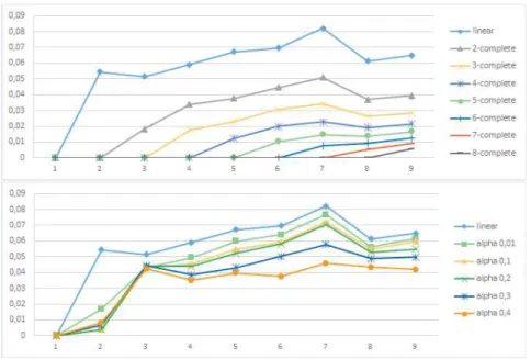
Results and interpretations Figure 3 indicates the computation time of all the explanation methods. This time takes in account every step of each method : the training of the models, the predictions necessary to calculate the influences, and the constitution of the correlated groups for the coalitional method. As ex-pected, the coalitionnal influences are much more efficient than the k-complete influences (less than 200s for the first ones compared to 700s for the other ones). The decrease in computation time for 9 attributes is explained by the important decrease in the mean number of instances. This makes each retraining faster to do, even if there are twice more subgroups to take into account. Figure 4 depicts the mean error score, aggregating the error score (Equation 9) of each explana-tion method for each of our 324 datasets. In this figure, the lowest curve is the

closest to the complete influence method, and thus is performing the best. As expected, the linear influence gives the worst results. This is explained by the fact it only considers single attributes, which is far from all the possible groups of attributes considered by the complete influence. The comparison between the k-completeinfluences and the coalitionnal influences (represented by their alpha parameters) is more delicate. Certainly, the k-complete influences outperform the other influences, in the majority of the cases, but with a high cost in execution time. Also, it does not mean the coalitionnal influences are less interesting for our case. They generate a smaller subset of groups of attributes while preserving an acceptable error score. Overall, the coalitional methods are not as satisfactory as the k-complete in term of effectiveness. But their comparatively very low ex-ecution time make them far more desirable when confronted with large datasets with an important number of attributes. Considering these results, it seems the k-completeinfluence is preferable with a relatively small k, and a dataset having few attributes, while the coalitional influence seems to become preferable with a higher number of attributes. Obviously, larger subgroups seems to increase the methods precision, but in the case of the coalitional method, their impact on computation time seems to be relatively small when compared to the per-formance gain. Besides, our study about the groups generated by the grouping algorithm shows that the number of groups stays relatively small, even for large alphas. As an example, for the datasets of 9 attributes, the mean size of the biggest generated group is 4, using an alpha of 0.4. This means that the coali-tional influence is working with far less information than the k-complete one. Studying the influence of different ways to generate the coalitions of attributes on the coalitional influence could be a good aim for the near future. With new methods, it could be possible to find more relevant groups, bettering the preci-sion of the explanation without an important computational cost. Moreover, it would be interesting to investigate overlapping attributes coalitions, using algo-rithms allowing for attributes to be in different coalitions, allowing to explore more subgroups if necessary.

5

Conclusion

We proposed in this paper a new way to explain the predictions of a single instance, aiming to reduce their cost of computation without losing too much information. The explaining methods we relate are a step further toward the goal of helping users employing machine learning tools. Our first experiment, in comparing the loss and gain methods, has led us to pinpoint flaws in their ini-tial design, especially the lack of consideration about attribute combinations. We proposed two adequate methods for prediction explanation, i.e. the k-complete and coalitional. These methods are faring better in term of calculation time, with a relatively small loss in accuracy. A short term perspective will be to in-vestigate the different subgroups generation methods and the results will help us to focus our efforts on the most promising candidates. A more long term per-spective is to implement a complete tool on this basis, with the goal of guiding

Fig. 3: Execution time, in milliseconds, of each explanation method depending on the number of attributes in the dataset. The mean number of instances is added for comparison.

Fig. 4: Error score between each explanation method and the complete influence depending on the number of attributes in the dataset.

a domain expert through the building and exploitation of a machine learning model. Another longer-term perspective also focuses on the problem of an ob-jective evaluation of explaining methods existing in the literature. Indeed, to the best of our knowledge, there is no benchmark for objectively evaluating these methods.

References

1. Altmann, A., Tolo¸si, L., Sander, O., Lengauer, T.: Permutation importance: a corrected feature importance measure. Bioinformatics 26(10), 1340–1347 (04 2010) 2. Casalicchio, G., Molnar, C., Bischl, B.: Visualizing the Feature Importance for

Black Box Models. arXiv e-prints (Apr 2018)

3. Datta, A., Sen, S., Zick, Y.: Algorithmic transparency via quantitative input influ-ence: Theory and experiments with learning systems. In: 2016 IEEE Symposium on Security and Privacy (SP). pp. 598–617 (May 2016)

4. Hall, M., Frank, E., Holmes, G., Pfahringer, B., Reutemann, P., Witten, I.H.: The weka data mining software: an update. ACM SIGKDD explorations newsletter 11(1), 10–18 (2009)

5. Henelius, A., Puolamaki, K., Bostr¨om, H., Asker, L., Papapetrou, P.: A peek into the black box : exploring classifiers by randomization. Data mining and knowledge discovery 28(5-6), 1503–1529 (2014), qC 20180119

6. Lundberg, S., Lee, S.I.: A unified approach to interpreting model predictions. In: NIPS (2017)

7. Quinlan, J.: Induction of decision trees. Machine Learning 1(1), 81–106 (Mar 1986) 8. Ribeiro, M.T., Singh, S., Guestrin, C.: ”why should i trust you?”: Explaining the predictions of any classifier. In: Proceedings of the 22Nd ACM SIGKDD Interna-tional Conference on Knowledge Discovery and Data Mining. pp. 1135–1144. KDD ’16, ACM, New York, NY, USA (2016)

9. Shapley, L.S.: A value for n-person games. Contributions to the Theory of Games (28), 307–317 (1953)

10. Shrikumar, A., Greenside, P., Kundaje, A.: Learning important features through propagating activation differences. In: Proceedings of the 34th International Con-ference on Machine Learning - Volume 70. pp. 3145–3153. ICML’17 (2017) 11. ˇStrumbelj, E., Kononenko, I.: Towards a model independent method for

explain-ing classification for individual instances. In: Song, I.Y., Eder, J., Nguyen, T.M. (eds.) Data Warehousing and Knowledge Discovery. pp. 273–282. Springer Berlin Heidelberg, Berlin, Heidelberg (2008)

12. Strumbelj, E., Kononenko, I.: An efficient explanation of individual classifications using game theory. J. Mach. Learn. Res. 11, 1–18 (Mar 2010)

13. Vanschoren, J., van Rijn, J.N., Bischl, B., Torgo, L.: Openml: Networked science in machine learning. SIGKDD Explorations 15(2), 49–60 (2013)