Simulated JWST data sets for multispectral and hyperspectral image fusion

OATAO is an open access repository that collects the work of Toulouse

researchers and makes it freely available over the web where possible

Any correspondence concerning this service should be sent

to the repository administrator:

tech-oatao@listes-diff.inp-toulouse.fr

This is a

publisher’s version published in:

https://oatao.univ-toulouse.fr/26226

To cite this version:

Guilloteau, Claire and Oberlin, Thomas and Berné, Olivier and

Habart, Émilie and Dobigeon, Nicolas Simulated JWST data sets for

multispectral and hyperspectral image fusion. (2020) The

Astronomical Journal, 160 (1). ISSN 0004-6256.

Open Archive Toulouse Archive Ouverte

Official URL :

Simulated JWST Data Sets for Multispectral and Hyperspectral Image Fusion

1

Institut de Recherche en Astrophysique et Planétologie(IRAP), University of Toulouse, France

2

Institut de Recherche en Informatique de Toulouse(IRIT), INPT-ENSEEIHT, University of Toulouse, France

3

ISAE-SUPAERO, University of Toulouse, France

4_{Institut d’astrophysique spatiale (IAS), University Paris-Sud, France} 5

Institut Universitaire de France, France

Received 2020 March 5; revised 2020 May 7; accepted 2020 May 11; published 2020 June 18

Abstract

The James Webb Space Telescope(JWST) will provide multispectral and hyperspectral infrared images of a large number of astrophysical scenes. Multispectral images will have the highest angular resolution, while hyperspectral images(e.g., with integral field unit spectrometers) will provide the best spectral resolution. This paper aims at providing a comprehensive framework to generate an astrophysical scene and to simulate realistic hyperspectral and multispectral data acquired by two JWST instruments, namely, NIRCam Imager and NIRSpec IFU. We want to show that this simulation framework can be resorted to assess the benefits of fusing these images to recover an image of high spatial and spectral resolutions. To do so, we make a synthetic scene associated with a canonical infrared source, the Orion Bar. We develop forward models including corresponding noises for the two JWST instruments based on their physical features. JWST observations are then simulated by applying the forward models to the aforementioned synthetic scene. We test a dedicated fusion algorithm we developed on these simulated observations. We show that the fusion process reconstructs the high spatio-spectral resolution scene with a good accuracy on most areas, and we identify some limitations of the method to be tackled in future works. The synthetic scene and observations presented in the paper can be used, for instance, to evaluate instrument models, pipelines, or more sophisticated algorithms dedicated to JWST data analysis. Besides, fusion methods such as the one presented in this paper are shown to be promising tools to fully exploit the unprecedented capabilities of the JWST.

Unified Astronomy Thesaurus concepts:Photodissociation regions(1223);Infrared astronomy(786);Spectroscopy (1558);Astronomy data analysis(1858);Astronomy data modeling (1859);Direct imaging(387)

1. Introduction

The James Webb Space Telescope (JWST) is an interna-tional collaboration space observatory involving NASA, the European Space Agency, and the Canadian Space Agency and is planned to be launched in 2021 (Gardner et al.2006). The four embedded instruments, the Near InfraRed Camera (NIRCam; Rieke et al.2005), the Near InfraRed Spectrograph (NIRSpec; Bagnasco et al. 2007), the Near InfraRed Imager and Slitless Spectrograph(NIRISS; Doyon et al.2012), and the Mid InfraRed Instrument(MIRI; Rieke et al.2015), will cover the infrared wavelength range between 0.6 and 28μm with an unprecedented sensitivity. The JWST will enable research on every epoch of the history of the universe, from the end of the dark ages to recent galaxy evolution, star formation, and planet formation. The scientific focuses of the JWST range from first light and reionization to planetary systems and the origins of life, through galaxies and protoplanetary systems. The JWST mission will observe with imagers and spectrographs. The imagers of NIRCam and MIRI will provide multispectral images (with low spectral resolution) on wide fields of view (with high spatial resolution), while the Integral Field Units (IFU) spectrometers of NIRSpec and MIRI will provide hyperspectral images (with high spectral resolution) on small fields of view (with low spatial resolution). Note that multi-spectral imaging and hypermulti-spectral imaging are generally referred to as multiband imaging and imaging spectroscopy, respectively, in the broad astronomy literature and, in particular, in the official JWST documentation. Conversely, in this study, we follow a more general convention adopted in

several scientific communities, e.g., signal & image processing, electron microscopy, remote sensing, and Earth observation. Indeed, throughout this paper we will refer to multispectral images to name images composed of a few dozen spectral bands, whereas hyperspectral images will stand for images composed of several hundred narrow and contiguous spectral bands. Consequently, multiband images will also refer to multispectral and hyperspectral images, indistinctly.

The aim of the present study is to assess the possible benefits of combining complementary observations, i.e., multispectral and hyperspectral data, of the same astrophysical scene to reconstruct an image of high spatial and spectral resolutions. If successful, such a method would provide IFU spectroscopy with the spatial resolution of the imagers. For the near-infrared range, which is the focus of this paper, this corresponds to an improvement by a factor of ∼3 of the angular resolution of NIRSpec IFU cubes, using the NIRCam images. Practically, this implies the possibility to derive integrated maps in spectral features (e.g., H recombination lines, ions, H2 lines) at the

resolution of NIRCam and at wavelengths where the latter instrument does not have anyfilter over the NIRSpec field of view (FOV). This may prove useful to derive high angular resolution maps of the local physical conditions, which requires the use of a combination of lines.

In the geoscience and remote sensing literature, the objective described above is usually referred to as“image fusion.” State-of-the-art fusion methods are based on an inverse problem formulation, consisting in minimizing a data fidelity term complemented by a regularization term (Simoes et al. 2015;

Wei et al. 2015). The data fidelity term is derived from a forward model of the observation instruments. The regulariza-tion term can be interpreted as prior informaregulariza-tion on the fused image. Simoes et al. (2015) proposed a total-variation-based prior and an iterative solving, while Wei et al. (2015) introduced a fast resolution by defining an explicit solution based on a Sylvester equation, thus substantially decreasing the computational complexity. Alternatively, Yokoya et al.(2012) proposed a method based on spectral unmixing called coupled nonnegative matrix factorization. Elementary spectral signa-tures, usually referred to as endmembers, and their relative proportions in the image pixels are estimated by an alternating non-negative matrix factorization (NMF) on the hyperspectral and multispectral images related through the observation model. In the particular context of JWST astronomical imaging, the first challenge of data fusion is due to the very large scale of the fused data, considerably larger than the typical sizes of data encountered in Earth observation. Indeed, a high spatio-spectral fused image in remote sensing is composed of approximately a few tens of thousands pixels and at most a few hundred spectral points versus a few tens of thousands pixels and a few thousand spectral points for a high spatio-spectral fused image in astronomical imaging. Moreover, another issue in astronomical image fusion is the complexity of observation instruments. Some specificities, such as the spectral variability of point-spread functions(PSFs), cannot be neglected because of the large wavelength range of the observed data. Therefore, remote sensing data fusion methods are not appropriate to fuse astronomical observation images. To address these issues, we discuss the relevance of a new fusion method specifically designed to handle JWST measurements.

To assess the relevance of fusing hyperspectral and multi-spectral data provided by the JWST instruments, a dedicated comprehensive framework is required, in the same spirit as the celebrated protocol proposed by Wald et al.(2005) to evaluate the performance of remote sensing fusion algorithms. This framework mainly relies on a reference image of high spatial and high spectral resolutions and the instrumental responses applied to this image to generate simulated observations. In the context of the JWST, the use of simulated observations with reference ground truth image is inevitable since,first, real data are not available yet and, second, only synthetic data allow the algorithm performances to be quantified. Thus, this paper aims at deriving an experimental protocol to evaluate the perfor-mance of fusion algorithms for JWST measurements. In the current study, the reference image of high spectral and high spatial resolutions, referred to as synthetic scene hereafter, has been synthetically created tofit the expected spectral properties of a photodissociation region (PDR; see definition in Section 2), covering a 31×31 arcsec2FOV between 0.7 and 28.5μm. This choice has been driven by our involvement in the JWST Early Release Science (ERS) program “Radiative Feedback from Massive Stars as Traced by Multiband Imaging and Spectroscopic Mosaics” led by Berné et al. (2017) and hereafter referred to as ERS 1288,6following the ID given by Space Telescope Science Institute(STScI). This choice is also motivated by our past expertise on this type of astrophysical source. However, one should keep in mind that the proposed simulation protocol and fusion method may in principle be applied to any kind of data set, with any type of source.

Besides, it is worth noting that the simulation of the hyperspectral and multispectral JWST data associated with this synthetic scene are much more complex than the forward models involved in the Wald’s protocol, mainly due to the specificities of the instruments mentioned above.

The paper is organized as follows. Section2 describes the specific structure of PDRs. Next, in Section 3, we make a synthetic spatio-spectral infrared PDR scene located in the Orion Bar with one spectral dimension(from 0.7 to 28 μm) and two spatial dimensions (each one ∼30″ wide or high). In Section 4, we properly define the forward models associated with the NIRCam Imager and NIRSpec IFU instruments. These are mathematical descriptions of the light path through the telescope and the instrument and include specificities such as wavelength-dependent PSFs, correlated noise, and spatial subsampling, among others. We apply these forward models to the PDR synthetic scene, to produce simulated NIRCam Imager and NIRSpec IFU near-infrared observations (0.7–5 μm) of the Orion Bar PDR. Finally, in Section 5, we perform symmetric data fusion between the NIRCam Imager short-wavelength(SW) channel (0.7–2.35 μm) and NIRSpec IFU simulated data to qualify the fused high spatio-spectral resolution image, and we evaluate the performance of this fusion scheme.

2. Photodissociation Regions

The present paper focuses on a synthetic scene of a PDR. We therefore provide in this section the general aspects of the concept of a PDR.

In the interstellar medium, photons from massive stars affect matter, which is found to be ionized, atomic, or molecular, each phase with different temperature and density. Transition regions between molecular clouds and ionized regions (HII)

are referred to as PDRs (Tielens & Hollenbach 1985). This concept of PDRs is applicable to many regions in the universe, such as the surface of protoplanetary disks(Adams et al.2004; Gorti & Hollenbach 2008; Champion et al.2017), as well as planetary nebulae (see, e.g., Bernard-Salas & Tielens 2005; Cox et al. 2016). More broadly, star-forming and planet-forming regions can be studied as PDRs (see, e.g., Tielens 2005; Goicoechea et al. 2016; Joblin et al. 2018), or even starburst galaxies (Fuente et al. 2005). Observations of nearby and spatially extended PDRs are essential to character-ize, as accurately as possible, their physical and chemical properties and to benchmark models. This can be done using spatio-spectral maps of PDRs in the mainfine-structure cooling lines of ions and atoms(in particular C+and O), or molecules such as H2(Habart et al. 2011; Bron et al. 2014), CO (Joblin

et al. 2018), or HCO+ (Goicoechea et al. 2016). From such observations and using PDR models(see a comparison of PDR models by Röllig et al.2007), temperature, electronic density, and pressure gradient maps with high spatial resolution can be extracted. Observations of rotational and rovibrational lines of H2 can also give clues about H2 formation processes (Bron

et al.2014). Finally, there are numerous studies dedicated to the evolution and photochemistry of polycyclic aromatic hydrocabons(PAHs), a family of large carbonaceous molecules that is ubiquitous in the universe, that are conducted in PDRs (see, e.g., Berné et al.2015; Peeters et al.2017).

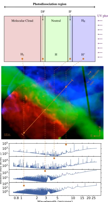
In star-forming regions, heating processes by extreme-UV (EUV, E<13.6 eV) and far-UV (FUV, E<13.6 eV) photons give PDRs a specific structure schematically represented in Figure 1. The H II layer is the region dominated by EUV

6

absorption and is composed of ionized gas. Its temperature is about 104K, and its density is a few hundred ions per cm3. FUV emissions penetrate deeper in the cloud and heat the neutral region, which is composed of neutral atomic gas. The temperature there is in the range of a few hundred to a few thousand kelvin, and its density is between 1000 and 104 hydrogen atoms per cm3. The limit between these two regions, where protons and electrons recombine, is called the ionization front (denoted IF in Figure 1). When the amount of FUV photons decreases sufficiently, hydrogen atoms can combine to form dihydrogen molecules (H2). This region is the molecular

cloud. The temperature there is between a few tens and a few hundred kelvin, and its density is about 104–106molecules per cm3. The limit where hydrogen atoms combine to become dihydrogen molecules, between the neutral region and the

molecular cloud, is defined as the dissociation front (denoted by DF in Figure1).

3. Synthesis of a PDR Scene: The Orion Bar 3.1. Approach

This section describes the synthesis of an astrophysical scene of infrared emissions of a PDR. Here we take the canonical PDR of the Orion Bar as a reference for the construction of this synthetic scene. This scene consists of a high spatio-spectral resolution 3D cube with two spatial dimensions and one spectral dimension. For convenience, the scene is not referred to as a 3D object, but rather as a 2D matrix whose columns contain the spectra associated with each spatial location. More precisely, letX denote the matrix corresponding to the synthetic scene where each column corresponds to the spectrum at a given location. This high spatial and high spectral resolution image is assumed to result from the product

( ) =

X HA, 1

whereH is a matrix of elementary spectra andA is the matrix of their corresponding spatial“weight” maps. The size, spectral range, and spatial FOV of these matrices are detailed in Table1. The underlying assumption of this model is that the data follow a linear model, i.e., the spectra composing the scene are linear combinations of spectra coming from “typical” regions. This choice has been adopted for several reasons. First, there is no spatio-spectral model of PDRs able to provide computed spectra with all signatures observable at near- and mid-infrared wavelengths(gas lines, PAHs bands, dust emission and scattered, etc.) and accounting for the complex spatial textures generally found in the observations(Goicoechea et al. 2016). The second reason is that the linearity of the mixture is a reasonable assumption at mid-IR wavelengths, where most of the emission is optically thin, except perhaps around 9.7μm, where silicate absorption may have an effect for large column densities (Weingartner & Draine 2001). In the near-IR wavelength domain studied in this paper some line emission is not optically thin, and thus the linear model used in this paper may not be fully correct. This applies in particular to the forest H2 lines around 2μm emanating from the PDR atomic and

molecular regions(seen in Figure 1, bottom panel). Extinction by dust along the line of sight in this wavelength range may also affect the line intensity by a nonlinear factor. Overall, this implies that the simple linear model will not provide a data cube that is physically validated at all positions and all wavelengths (providing such data would be a difficult task); however, that general statistic of the data set is likely to be realistic. At least, it is the best that can be done at this stage.

An additional advantage of definingX as a matrix product is related to its computing storage: the full matrix is expected to be quite large, and simply impossible to store in memory. Instead, adopting such a decomposition, only the underlying model factorsH andA need to be stored, hence significantly reducing the occupied memory. The following sections describe the choice of the elementary signatures inH and their spatial mapping inA.

Figure 1. PDR. Top: PDR synthetic morphology with, from right to left, ionized or H II region (H II), ionization front (IF), the neutral region,

dissociation front(DF), and the molecular cloud. Middle: PDR as seen by HST (in blue; Bally 2015), the Spitzer Space Telescope (Fazio et al. 2004) and ALMA(in red; Goicoechea et al.2016). Bottom: four synthetic spectra from 0.7 to 28μm of four different regions from the PDR with, from top to bottom, the ionized region, the ionization front, the dissociation front, and the molecular cloud(see text for details).

3.2. Elementary SpectraH

The elementary spectra composing the matrixH have been computed within the framework of the ERS 1288 program (Berné et al. 2017). A more detailed description of how they have been calculated will be provided in a paper aiming at describing the scientific objectives of this ERS 1288 program. This matrixH is composed of k=4 spectra corresponding to four regions of a PDR as depicted in Figure1: the HIIregion, the ionization front, the dissociation front, and the molecular cloud. These spectra have been computed individually for each region, using the Meudon PDR code for the contribution from molecular and atomic lines(Le Petit et al.2006), the CLOUDY code for the ionized gas (Ferland et al. 1998), the PAHTAT model(Pilleri et al.2012), and results from the decomposition of Foschino et al. (2019) for the PAH emission and the DUSTEM model for the contribution from the dust continuum (Compiègne et al. 2011). The physical parameters used for these models correspond to those of the Orion Bar, which is a well-studied region. Absolute calibration of the total spectrum resulting from the sum of the four different regions has been crossed-check with existing observations of the Orion Bar (ISO, Spitzer), so as to confirm that the total spectra are realistic in terms of flux units. However, we emphasize that the individual spectra of the different regions, obtained by making simple assumptions in particular on the properties of dust(e.g., same property in all the regions), the radiative transfer, and the calculation of the emission line, are probably not realistic. The ratio of gas lines to the dust continuum is probably under-estimated by large factors (>10) in the atomic and molecular PDR owing to an underestimation of dust emission and an overestimation of the lines of H2not corrected for extinction.

As mentioned above, while this could be an issue when trying to interpret the synthetic data from a detailed physical point of view, this is not a limitation for the data fusion exercise, since the overall statistical properties are likely to be correct.

3.3. Abundance MapsA

Since the spectra inH carry the flux information, spatial abundance maps in the matrixA correspond to normalized between 0 and 1 textures. In this work they are derived from real data from the Hubble Space Telescope (HST) and the Atacama Large Millimeter/submillimeter Array (ALMA). They have been rotated by −48° to obtain a plane-parallel morphology reminiscent of the conceptual structure described in Figure 1. The layout resulting from this rotation has been chosen so that the fusion results reported in Section 5 can be depicted while saving space. This is also because the FOV of the currently planned observation of the ERS 1288 program will be perpendicular to the IF/DF, i.e., corresponding to a

horizontal cut in the rotated images. The chosen FOV for the synthesis of the texture maps from the observations is a 31×31 arcsec2 square centered on coordinates R.A.= 5:35:20.0774, decl.=−5:25:13.785 in Orion. The textures associated with the four spectral components are described below according to their corresponding regions.

3.3.1. Ionization Front and HIIRegion

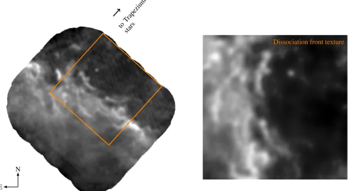
To build an accurate spatial representation of the HIIregion and the ionization front, we have resorted to the Orion Bar image obtained by the narrowband filter centered at 656 nm (Hα emission line) of the WFC3 instrument aboard the HST (Figure 2). This image was taken as part of the observing proposal led by Bally(2015). This image provides an accurate view of the morphology of the HII region and the ionization front combined(Tielens2005).

After cropping and rotating, we have separated the ionization front and H II region in the observed image. As the brightness of the ionization front is comparable to the brightest regions in the HIIregion, a thresholding on the raw image does not isolate efficiently the ionization front from the plasma cloud. However, unlike the H II region, the front appears as a sharp line where the gradient of the image is high. Therefore, the location of the pixels in the image belonging to the IF can be easily recovered from the pixel-scale horizontal gradient of the image, which can also be computed using a Sobelfilter (Gonzalez et al. 2002). Thus, the latter is thresholded to create a mask around the pixels with highest gradient magnitudes. The smallest connected components(smaller than 10,000 pixels) are then removed to delete high gradient values related to small objects in the image and thus not related to the IF. Finally, the original HST image is termwise multiplied by this mask and slightly smoothed by a Gaussian kernel with an FWHM of 4.7 pixels. This allows the contribution to be extracted from the IF only, andfinally an IF image to be obtained (see Figure2).

Once the ionization front is removed from the original image, the gap is expended by a morphological dilation with a 20-pixel-diameter disk and filled using a standard inpainting technique (Damelin & Hoang 2018). This process fills the missing part by selecting similar textures available outside the mask. The result is shown in Figure 2. Both images are then up-sampled to the resolution of the JWST NIRCam Imager instrument by bi-cubic spline interpolation with a 1.25 up-sampling factor.

3.3.2. Dissociation Front

The texture map related to the dissociation front is derived from an image of HCO+ (4–3) emission observed by

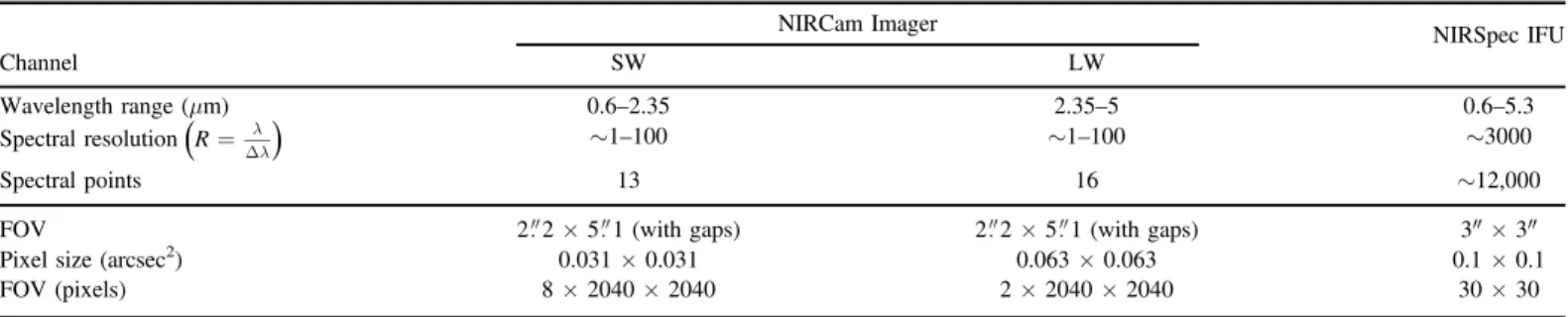
Table 1

Properties of the Synthetic Scene of the Orion BarX Presented in Figure6and the Underlying Elementary Spectra and Spatial“Weight” Matrices, Respectively Denoted asH andA

X H A

Wavelength range(μm) 0.7–28.5 0.7–28.5 L

Spectral resolution

(

)

FOV 31″×31″ L 31″×31″

Pixel size(arcsec2) 0.031×0.031 L 0.031×0.031

Goicoechea et al.(2016) with ALMA; see Figure3. According to the authors, this map locates well the H/H2transition and is

consequently used here to define the dissociation front of this PDR.

After rotation and cropping, the high textured zone in the right part of the chosen area is extracted by thresholding. Then, it is slightly smoothed by a Gaussian kernel with a 2.3-pixel FWHM. The remaining part, less structured, is much more

Figure 2.(a) HST image of 656 nm Hα emission line in the Orion Bar (Bally2015) and the chosen FOV (orange box). (b) Extracted ionization front texture. (c) Extracted HIIregion texture. Normalized scale(black: 0; white: 1), centered in R.A.=5:35:20.0774, decl.=−5:25:13.785.

Figure 3.Left: ALMA image of HCO+(4–3) line peak in the Orion Bar (Goicoechea et al.2016) and the chosen FOV (orange box). Right: normalized texture for the dissociation front abundance map(black=0, white=1).

smoothed thanks to a Gaussian kernel with a 9.4-pixel FWHM to remove visible noisy stripes due to the ALMA data acquisition process.

Then, the smoothed image is up-sampled to the resolution of the NIRCam Imager instrument by bi-cubic spline interpolation with an up-sampling factor of 5 and normalized. The resulting texture is shown in the right panel of Figure3.

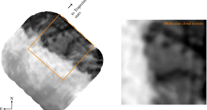
3.3.3. Molecular Cloud

The molecular cloud texture map has also been extracted from an ALMA image(Goicoechea et al.2016). The CO (3–2) emission line is commonly used as a tracer of the molecular cloud. As explained in the previous section, the area in the orange box in Figure 4 (left) has been chosen to match the textures maps of the three previous regions. The stripes due to the ALMA data acquisition process are clearly noticeable over the full FOV. Therefore, after rotation, the image is strongly smoothed with a Gaussian kernel with an 11-pixel FWHM to remove these unwanted stripes, identified as noise. The smoothed image is finally up-sampled to the resolution of the NIRCam Imager instrument by bi-cubic spline interpolation (with an up-sampling factor of 5) and normalized. The resulting texture is shown in the right panel of Figure4.

4. JWST Instruments Forward Model

In this section, we derive a simple yet sound mathematical model of two instruments embedded in the JWST, namely, NIRSpec IFU and NIRCam Imager. A more advanced modeling was previously conducted by the teams in charge of the JWST Exposure Time Calculator (ETC) at the STScI (Pontoppidan et al.2016). The ETC is a tool for astronomers to simulate data acquisition and to compute signal-to-noise ratios (S/Ns) for all JWST observing modes and instruments. This

tool models the full acquisition process (groups, integration ramps) and noise for astrophysical scenes composed of complex spectra and several extended (ellipses) or point sources. However, the ETC tool exhibits two major limitations in the context of the work targeted in this paper, i.e., within a fusion perspective. First, currently there is no stable version of the ETC that provides simulated measurements for complex spatio-spectral 3D scenes such as the astrophysical scene described in Section3. Note that we are currently working with STScI to overcome this limitation, e.g., by using the linear properties of the synthetic scene described in Section 3. The second reason is that the forward models involved in the considered fusion method are required to be explicit and hence less advanced than those provided by the ETC(see Section7). As a consequence, we derived explicit forward models capitalizing on the information available in the ETC as a reference. The models associated with the two instruments under consideration, supplemented by a suitable noise model-ing, are described in what follows.

4.1. NIRCam Imager

The near-infrared camera NIRCam Imager aboard the JWST will observe space from 0.6 to 5 μm with three possible data acquisition modes: imaging, coronagraphy, and slitless spectrosc-opy. The observing mode studied in this paper is the imaging mode. It will provide multispectral images on widefields of view (2 2×5 1, separated on two adjacent modules). This instru-ment covers the 0.6–5 μm wavelength range simultaneously through two channels, the SW channel between 0.6 and 2.3μm and the long-wavelength(LW) channel between 2.4 and 5 μm, via lm=29 extrawide, wide, medium, and narrow filters. Each

channel, SW or LW, acquires images composed of pmpixels with

pixel sizes of 0.031×0.031 arcsec2and 0.063×0.063 arcsec2,

Figure 4.Left: ALMA image of the CO(3–2) line peak in the Orion Bar (Goicoechea et al.2016) and the chosen FOV (orange box). Right: normalized texture molecular cloud abundance map(black=0, white=1).

respectively. The main technical features are summarized in Table2.

The proposed mathematical model of the NIRCam Imager detailed in this section is derived to reflect the actual light path through the telescope and the instrument and the corresponding spatial and spectral distortions. The optical system of the telescope and the instrument, and more specifically mirrors, disturb the incoming light and its path. The effect on the detector and therefore on the observed image is a spatial spread of the light arising from the sky, resulting in a blurring of the spatial details. This blurring depends on the wavelength λ (in meters) of the incoming light and the JWST primary mirror diameter D(in meters) such that the effective angular resolution θ (in radians), i.e., the ability to separate two adjacent points of an object, is limited by diffraction. After the optics and the mirrors, the light passes through bandpass filters defined by specific wavelength ranges.

These two main degradations (i.e., spatial blurring and spectralfiltering) can be expressed with closed-form mathema-tical operations successively applied to the astrophysical sceneX. First, the light-spread effect due to the optical systems is modeled as a set of spectrally varying 2D spatial convolutions, denoted  . The corresponding PSFs, calculated with the(·)

online tool webbpsf (Perrin et al. 2012), are wavelength dependent, and the FWHM of the spread patch grows linearly with the wavelength. This dependency is illustrated in the top panel of Figure 5, which exhibits the significantly different patterns of four PSFs associated with four particular wave-lengths. The following spectralfiltering step, which degrades the spectral resolution of the scene, can be modeled as multi-plications by the transmission functions of the NIRCam Imager filters (Space Telescope Science Institute (STScI)2017a). This operation can be formulated through a product by the matrixLm,

whose rows are defined by these transmission functions. Therefore, the noise-free multispectral image ¯Ym composed of

lm(=lh) spectral bands and pmpixels can be written as

¯ _{= ( ) ( )}

Ym Lm X . 2

Note that a similar approach was followed by Hadj-Youcef et al.(2018) to derive the forward model associated with the imager embedded in MIRI.

4.2. NIRSpec IFU

The near-infrared spectrograph NIRSpec IFU embedded in the JWST will perform spectroscopy from 0.6 to 5.3μm at high

Table 2

Main Technical Features of NIRCam Imager and NIRSpec IFU Considered in This Study

NIRCam Imager _{NIRSpec IFU}

Channel SW LW

Wavelength range(μm) 0.6–2.35 2.35–5 0.6–5.3

Spectral resolution

(

)

Spectral points 13 16 ∼12,000

FOV 2 2×5 1 (with gaps) 2 2×5 1 (with gaps) 3″×3″

Pixel size(arcsec2_{) 0.031×0.031 0.063×0.063 0.1×0.1}

FOV(pixels) 8×2040×2040 2×2040×2040 30×30

(R∼3000), medium (R∼1000), or low (R∼100) spectral resolution through four observing modes. The ERS 1288 program proposed by Berné et al.(2017) will rely on the IFU with high-resolution configuration. It will provide spectro-scopic (also called hyperspectral) images on small fields of view(3×3 arcsec2). Data acquisition on the wavelength range is covered by several disperser-filter combinations with similar features. Although unprecedented, the spatial sampling of the IFU is about 9 times less than NIRCam Imager with a 0.1×0.1 arcsec2 pixel size. The main technical features of NIRSpec IFU are summarized and compared with NIRCam Imager features in Table 2.

As for NIRCam Imager, the light path from the observed scene to the detector through the telescope and the instrument can be formulated thanks to simple mathematical operations while preserving physical accuracy of the model. At first, the light is spread by the optical system, depending on its wavelength and JWST primary mirror. Second, the path through the disperser-filter pair attenuates the light. Finally, this light comes on the detector, which can provide ∼12,000 spectra over a 30×30 pixel2spatial area.

The optical system distortion effect of the telescope and the instrument on the light is, as for NIRCam Imager, modeled as a set of 2D spatial wavelength-dependent convolutions denoted

(·)

 with PSFs illustrated in the bottom panel of Figure5. The light attenuation induced by the disperser-filter pair is a matrix multiplication byLh, whose diagonal is the combination of

both transmission functions(Space Telescope Science Institute (STScI)2017b). Besides attenuation, the physical gaps between NIRSpec IFU detectors involve holes in spectra. These holes are modeled by a null transmission at the corresponding wavelengths. The spatial response of the detector is seen as a downsampling operatorS, which keeps 1 pixel over a 0.1×0.1 arcsec2 area, after averaging pixels over this area. Finally, the noise-free hyperspectral image ¯Yh composed of lh

spectral bands and ph=pmpixels can be written as

¯ _{= ( ) ( )}

Yh Lh X S. 3

4.3. Noise Modeling

This section models the noise associated with NIRCam Imager and NIRSpec IFU that corrupts the noise-free images ¯Ym

and ¯Yh to yield the simulated imagesYm andYh, respectively.

This composite model relies on the most commonly used hypotheses on the nature of the space observation noise and on more specific assumptions regarding the JWST detectors. The proposed model neglects some other sources of noise that are more difficult to characterize, e.g., those related to cosmic rays and background. A more realistic and exhaustive noise modeling is provided by the STScI via the ETC(Pontoppidan et al.2016).

4.3.1. Quantum Noise

Since the detectors are photon-counting devices, the particular nature of light emission conventionally induces observations that obey a Poisson distribution  y whose mean is equal to the( ¯) photon count ¯y. In a high-flux regime, i.e., when the photon count ¯y is typically higher than 20, this Poisson process can be approximated by an additive heteroscedastic Gaussian noise

( ¯ ¯)

 y y, whose mean and variance is the photon count ¯y. In the particular context of this work, we will assume that the observations follow this high-flux regime, which is a reasonable assumption especially for a very bright source such as the Orion

Bar. As a consequence, in practice, the incoming flux ¯y in a given pixel and a given spectral band will be corrupted by a random variable drawn from y y( ¯ ¯), . This model is commonly used to define noise in astronomical imaging (Starck & Murtagh 2006).

4.3.2. Readout Noise

The main source of corruptions induced by the detectors is a readout noise, which is modeled as an additive, centered, colored Gaussian noise. The correlation between two measure-ments at given spatial and spectral locations of the observed multiband image can be accurately characterized after unfold-ing the 3D data cube onto the detector plan. Indeed, the JWST and the ETC documentations(Pontoppidan et al.2016) provide a set of matrices reflecting the expected correlations between measurements at specific positions in the plan of the detectors associated with NIRCam Imager and NIRSpec IFU. These correlation matrices are functions of intrinsic characteristics of the readout pattern, such as the integration time, the number of frames, and the number of groups(Rauscher et al.2007). For a given experimental acquisition setup, the covariance matrix of the additive Gaussian readout noise could be computed after a straightforward ordering of these correlations with respect to the reciprocal folding procedure. Alternatively, this colored Gaussian noise can be added to the unfolded multiband images with a covariance matrix directly defined by the correlations expressed in the detector plan and specified by Pontoppidan et al. (2016). Complementary information regarding the NIRCam Imager and NIRSpec IFU readout noises is given in what follows.

NIRCam Imager readout noise.—The spectral bands of the multispectral image are acquired successively such that the incident image on the detector corresponds to a 2D spatial image in a given spectral. Hence, the induced readout noise is only spatially correlated and can be generated for each spectral band independently. Finally, the covariance matrix describing the spatial correlation of the additive Gaussian noise is computed thanks to the correlation patterns in the detector plan discussed above.

NIRSpec IFU readout noise.—Contrary to the NIRCam Imager detector, the plan of the NIRSpec IFU detector consists of a 1D spatial and 1D spectral image. More precisely, the optical system of NIRSpec IFU is composed of a slicer mirror array that slices the observed FOV into 0 1-wide strips (corresponding to the NIRSpec IFU pixel size) to realign them in one dimension along one detector axis (Space Telescope Science Institute (STScI) 2017c). For each spatial pixel, its spectrum is dispersed along the second detector axis. As a consequence, the corresponding readout noise is not indepen-dent from one spectral band to another. Thus, as previously explained above, this noise can be generated with a covariance matrix driven by the readout pattern features discussed above and added to the unfolded counterpart of the observed hyperspectral image after projection onto the detector plan.

4.3.3. Zodiacal Light, Background, and Cosmic Rays According to JWST documentation (Kelsall et al. 1998; Pontoppidan et al.2016), the emissions from the zodiacal cloud of the solar system and of the Milky Way, as well as emission from the telescope, are assumed to be negligible for bright sources, up to 5 μm. Furthermore, the JWST pipeline is

designed to remove 99% of cosmic-ray impact effects. These noise sources are thus neglected in this work. Note that a comprehensive model of background noise and cosmic-ray impacts has been developed by the STScI for the ETC.

5. Experiments

5.1. Simulating Observations Using JWST Forward Models This section capitalizes on the forward models of NIRCam Imager and NIRSpec IFU and the associated noise model proposed in Section4to simulate observations associated with the synthetic astrophysical scene generated according to the framework introduced in Section 3. To adjust the character-istics of the noise, we rely on the integration times as planned by the ERS 1288 program of Berné et al.(2017). The observing parameters of this program can be downloaded publicly through the Astronomer’s Proposal Tool (APT) provided by the STScI. The characteristics of the resulting simulated multispectral and hyperspectral images, respectively denoted asYm andYh, are summarized in Table 3. The FOV of the

resulting simulated imageYmcorresponds to about 1/16 of the

total NIRCam Imager FOV since the synthetic scene is smaller than the actual full NIRCam Imager FOV. On the other hand, the FOV of the simulated hyperspectral imageYhcorresponds

to a mosaic of 10×10 NIRSpec IFU FOVs. These simulated multispectral and hyperspectral images are shown in Figure6. To illustrate the contents of the simulated data set, we present red–green–blue (RGB) colored compositions of the images, as well as spectra extracted at specific positions, for the scene and simulated observations (see Figure 6 for details of the composition). The simulations show how the instruments degrade the spectral and spatial resolution of the fully resolved synthetic astrophysical scene. More precisely, for the multi-spectral observations, the RGB composition shows less contrast, due to the loss of spectral information due to the wide filters. The hyperspectral data are clearly less spatially resolved, and the spectra exhibit a high level of noise. Overall, for the considered realistic scene of the Orion Bar, which is a bright source, it is worth noting that the S/N remains high for most parts of the images and spectra.

5.2. Fusion of Simulated Observations 5.2.1. Method

The synthetic scene and the simulated observed NIRCam Imager and NIRSpec IFU images have been generated to assess the performance of a dedicated fusion method we have developed (Guilloteau et al. 2019). We refer the reader to the latter paper for full details about the method, but we provide below the main characteristics of the fusion algorithm. The fusion task is formulated as an inverse problem, relying on

the forward models specifically developed for the JWST NIRCam Imager and NIRSpec IFU instruments in Section4. More precisely, the fused product ˆX is defined as a minimizer

of the objective function(·)given by

( ) ( ) ( ) ( ) ( ) ( )    s s j j = - + -+ +  X Y L  X Y L X S X X 1 2 1 2 , 4 m 2 m m F 2 h 2 h h spe spa

where · F is the Frobenius norm. The two first terms are

referred to as data fidelity terms, and sm2 and s2h are their

respective weights associated with the noise level in each observed imageYmandYh. The noisier they are, the greater s2m

or sh2, and the less significant the related data fidelity term. The

complementary terms jspe(X) and jspa(X) are, respectively,

spectral and spatial regularizations summarizing a priori information on the expected fused image. This general approach has been adopted by a large number of methods already proposed in the literature, e.g., for remote sensing and Earth observation (Simoes et al. 2015; Wei et al. 2015). However, in this paper, the considered forward models account for JWST instrument specificities, in particular spectrally variant spatial blurs, which make all previous approaches inoperable and require the development of a dedicated fusion method.

In the approach advocated by Guilloteau et al. (2019), the spectral regularization jspa(·) in Equation (4) relies on the

prior assumption that the spectra of the fused image live in a low-dimensional subspace, whereas the spatial regularization jspa(·) promotes a smooth spatial content. Due to the

high-dimensionality of the resulting optimization problem, its solution cannot be analytically computed but requires an iterative procedure. To get a scalable and fast algorithm able to handle realistic measurements, Guilloteau et al. (2019) proposed two computational tricks: (i) the problem is formulated in the Fourier domain, where the convolution operators(·) and(·)can be efficiently implemented, and (ii) in a preprocessing step the JWST forward models are computed in the lower-dimensional subspace induced by the spectral regularization, which leads to sparse and easily storable operators. By combining these two tricks, the final algorithmic procedure minimizing(·)saves about 90% of the computational time with respect to a naive implementation.

5.2.2. Results

In this work, we perform the fusion task on a subset of the simulated multi- and hyperspectral observed images. This choice has beenfirst guided by the observing strategy currently considered in the ERS 1288 observing program for the Orion Bar(Berné et al.2017). In practice, as depicted in Figure6, the FOV used for fusion(orange boxes on the right-hand side) is limited to a 2.7×27 arcsec2cut across the bar, representing a mosaic of nine NIRSpec IFUs FOVs. Second, as the SW and LW channels of the NIRCam Imager present distinct spatial sampling properties, we restrict the test of the fusion algorithm to the spectral range of the shorter wavelengths, between 0.7 and 2.35μm, where the ratio of spatial resolution between imager and spectrometer is largest (i.e., where the fusion is most difficult). In the end, the objective is to fuse a

Table 3

Properties of the Simulated Observed NIRCam Imager and NIRSpec IFU Mosaic Images, Namely,YmandYh

Ym _Yh Channel SW LW Wavelength range(μm) 0.7–2.35 2.35–5.2 0.7–5.2 Spectral points 13 16 11586 FOV(arcsec2_{) 30×30 30×30 30×30} FOV(pixels2_{) 1000×1000 500×500 310×310}

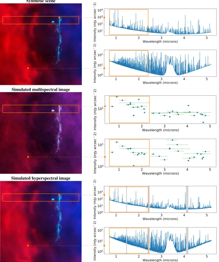
Figure 6.Left(from top to bottom): RGB compositions of the synthetic PDR scene, the simulated NIRCam Imager multispectral image, and the simulated NIRSpec IFU hyperspectral image. Red: H2emission line peak intensity at 2.122μm (narrow filter F212N for the multispectral image); green: H recombination line peak intensity at 1.865μm (narrow filter F186N for the multispectral image); blue: Fe+emission line peak intensity at 1.644μm (narrow filter F164N for the multispectral image). The observed FOV and spectral range considered in the fusion problem are represented by the orange boxes. Right: two spectra from 0.7 to 5 μm associated with 2 pixels of each image on the left. From top to bottom, thefirst two are original spectra from the synthetic scene with about 12,000 points, the following two are observed spectra from the multispectral image provided by NIRCam Imager forward model with 29 spectral points, and the last two are calibrated observed spectra from the hyperspectral image provided by NIRSpec IFU forward model with about 11,000 points. Physical gaps in NIRSpec IFU detectors are specified in gray. Intensities are plotted in a logarithmic scale. Thefirst, third, and fifth spectra are dominated by ionization front and ionized region emissions, while the second, fourth, and sixth are dominated by dissociation front and molecular cloud emissions.

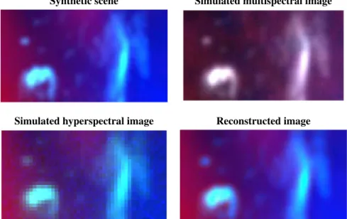
Figure 7.Top(from top to bottom): RGB compositions of the synthetic PDR scene, the simulated NIRCam Imager multispectral image, the simulated NIRSpec IFU hyperspectral image—following, respectively, the NIRCam Imager and the NIRSpec IFU forward models—and the fused image of high spatio-spectral resolution. Red: H2emission line peak intensity at 2.122μm; green: H recombination line peak intensity at 1.865 μm; blue: Fe+emission line peak intensity at 1.644μm. Bottom: calibrated spectra, with about 5000 points, related to 2 pixels of the images above. Thefirst plot shows spectra dominated by ionization front emissions, and the second plot shows spectra dominated by dissociation front and molecular cloud emissions. The two plots display the associated simulated hyperspectral spectrum following the NIRSpec IFU forward model, the original spectrum to be recovered, and the reconstructed spectrum, retrieved by the fusion algorithm. Zoom-in parts are 3 times magnified. Intensities are plotted in a logarithmic scale.

13×90×900 pixel simulated multispectral image and a 5000×28×279 pixel simulated hyperspectral image, as illustrated in Figure7.

The fused image depicted in Figure7has been obtained after about 2000 s of preprocessing(dedicated to the pre-computa-tion of the JWST forward models in the lower-dimensional subspace) and 20 s of iterative minimization of the objective function  . Qualitatively and generally speaking, the(·) reconstruction is excellent from spectral and spatial points of view. Regarding the spectra, the fusion is very good for pixels that are located on smooth spatial structures. Efficient denoising can be observed since reconstructed spectra show much less noise than the simulated NIRSpec IFU hyperspectral image. However, in regions with significant and sharp variations of the intensity at small spatial scales (such as the ionization front), the fusion procedure appears to be less accurate. This is likely due to the chosen spatial regularization, which tends to promote smooth images and therefore distributes the flux over neighboring pixels. This issue is currently under investigation to provide a better regularization able to mitigate this effect. Similar conclusions can be drawn when analyzing the spatial content of the fused image, as illustrated in Figure8. Overall, the reconstruction is very good, and a significant denoising is also observed. The gain in resolution of the reconstructed image with respect to the hyperspectral image is clearly noticeable, but thin structures, such as the ionization front, are smoother than in the original simulated astrophysical scene. Again, this is likely due to the regularization.

We now turn to a more quantitative analysis of the performance of the fusion method. To do so, we consider the reconstruction S/N of the fused image X with respect to the corresponding actual sceneX. It is expressed as

( ) ⎛ ⎝ ⎜ ⎞ ⎠ ⎟     = -X X X S N 10 log₁₀ 2 . 5 2 F 2

The reconstruction S/N reached by the proposed fusion procedure is compared to the S/N associated with an up-sampled counterpart of the observed hyperspectral image obtained by a simple bandwise bi-cubic spline interpolation

to the resolution of the synthetic scene. The resulting S/Ns are 18.5 and 10.6 for the fused product and the up-sampled observed hyperspectral image, respectively. This means that spatial and spectral contents are much more accurately reconstructed by the fusion process proposed by Guilloteau et al.(2019). Such results underline the benefit of data fusion compared with considering only the observed hyperspectral image, discarding the information brought by the multispectral image.

5.2.3. Perspectives for Fusion Methods in the Context of the JWST Mission

Overall, the results of data fusion performed on simulated multispectral and hyperspectral JWST images show high-quality spectral and spatial reconstruction of the scene. Most of the spectral and spatial details lost either in the multispectral or in the hyperspectral image are recovered in the fused product. Such results support further investigations on this fusion method, with great promises of application on real data. One preliminary step to be achieved concerns a more comprehen-sive performance assessment. It is indeed necessary to evaluate the benefit of the the fusion procedure when dealing with simulated observations obtained from the JWST scientific team through the ETC tool, with possibly the synthesis of the same 3D complex scene described in Section3. This is a project that we are currently undertaking with STScI. Current limitations of the methods we have identified concern the unsatisfactory reconstruction of sharp structures in the synthetic scene, due to the chosen spatial regularization, which promotes a smooth spatial content in the fused product. Considering a regulariza-tion term in the objective funcregulariza-tion(·)defined in Equation (4) is necessary not to overfit the noise in the observed images. Future works should address this issue by designing a tailored regularization.

6. Conclusion

In this work we built a synthetic scene of a PDR located in the Orion Bar with high spatio-spectral resolution. This scene has been created according to current models with simulated

spectra and spatial maps derived from real data. Forward models of two instruments embedded on the JWST, namely, NIRCam Imager and NIRSpec IFU, were developed and used to simulate JWST observations of the Orion Bar PDR. These simulated data were used to assess the performance of a fusion method we developed. The results showed to be promising for recovering spectroscopic and spatial details that were lost in the simulated NIRCam Imager and NIRSpec IFU observations. This suggested that image fusion of JWST data would offer a significant enhancement of scientific interpretation. However, improvements of the fusion method are still required, in particular to mitigate the effect of the regularization. Moreover, the noise characteristics assumed in this study relied on theoretical models and specifications implemented in the ETC. More realistic noise models are expected to be available after JWST launch. Improving the currently assumed noise model is thus left for future work. Finally, the authors would like to stress that they are in contact with the ETC team at the STScI. Their objectives are twofold: (i) to benefit from current and future improvements of the ETC to better assess the performance of the fusion method, and (ii) to make the proposed method for synthesis of an astrophysical scene more versatile for a possible implementation into the ETC.

The authors thank K. Pontoppidan for his feedback on the ETC and the JWST documentation and the members of the core team of ERS project“Radiative Feedback from Massive Stars as Traced by Multiband Imaging and Spectroscopic Mosaics” for providing the spectra used to create the simulated data sets. They thank A. Albergel, F. Orieux, and R. Abi Rizk for fruitful discussions regarding this work. Part of this work has been supported by the ANR-3IA Artificial and Natural Intelligence Toulouse Institute(ANITI), the French Programme Physique et Chimie du Milieu Interstellaire (PCMI) funded by the Conseil National de la Recherche Scientifique (CNRS), and Centre National d’Études Spatiales (CNES).

ORCID iDs

Claire Guilloteau https://orcid.org/0000-0001-5800-9647 Thomas Oberlin https://orcid.org/0000-0002-9680-4227 Olivier Berné https://orcid.org/0000-0002-1686-8395 Émilie Habart https://orcid.org/0000-0001-9136-8043 Nicolas Dobigeon https://orcid.org/0000-0001-8127-350X

References

Adams, F. C., Hollenbach, D., Laughlin, G., & Gorti, U. 2004,ApJ,611, 360 Bagnasco, G., Kolm, M., Ferruit, P., et al. 2007,Proc. SPIE,6692, 66920M Bally, J. 2015, The First Ultraviolet Survey of Orion Nebula’s Protoplanetary

Disks and Outflows, HST Proposal,13419

Bernard-Salas, J., & Tielens, A. G. G. M. 2005,A&A,431, 523

Berné, O., Habart, E., Peeters, E., et al. 2017, Radiative Feedback from Massive Stars as Traced by Multiband Imaging and Spectroscopic Mosaics, JWST Proposal,1288

Berné, O., Montillaud, J., & Joblin, C. 2015,A&A,577, A133 Bron, E., le Bourlot, J., & le Petit, F. 2014,A&A,569, A100 Champion, J., Berné, O., Vicente, S., et al. 2017,A&A,604, A69 Compiègne, M., Verstraete, L., Jones, A., et al. 2011,A&A,525, A103 Cox, N. L. J., Pilleri, P., Berné, O., Cernicharo, J., & Joblin, C. 2016,MNRAS:

Letters,456, L89

Damelin, S. B., & Hoang, N. S. 2018,Int. J. Mathematics and Mathematical Sciences, 2018, 3950312

Doyon, R., Hutchings, J. B., Beaulieu, M., et al. 2012, Proc. SPIE, 8442, 84422R

Fazio, G. G., Hora, J. L., Allen, L. E., et al. 2004,ApJS,154, 10 Ferland, G. J., Korista, K. T., Verner, D. A., et al. 1998,PASP,110, 761 Foschino, S., Berné, O., & Joblin, C. 2019,A&A,632, A84

Fuente, A., García-Burillo, S., Gerin, M., et al. 2005,ApJL,619, L155 Gardner, J. P., Mather, J. C., Clampin, M., et al. 2006,SSRv,123, 485 Goicoechea, J. R., Pety, J., Cuadrado, S., et al. 2016,Natur,537, 207 Gonzalez, R. C., Woods, R. E., & Masters, B. R. 2002,JBO,14, 029901 Gorti, U., & Hollenbach, D. 2008,ApJ,690, 1539

Guilloteau, C., Oberlin, T., Berné, O., & Dobigeon, N. 2019, arXiv:1912. 11868

Habart, E., Abergel, A., Boulanger, F., et al. 2011,A&A,527, A122 Hadj-Youcef, M. E. A., Orieux, F., Fraysse, A., & Abergel, A. 2018, 26th Proc.

European Signal Process. Conf.(EUSIPCO), hal-01952286, https: //hal-centralesupelec.archives-ouvertes.fr/hal-01952286

Joblin, C., Bron, E., Pinto, C., et al. 2018,A&A,615, A129 Kelsall, T., Weiland, J. L., Franz, B. A., et al. 1998,ApJ,508, 44 Le Petit, F., Nehmé, C., le Bourlot, J., & Roueff, E. 2006,ApJS,164, 506 Peeters, E., Bauschlicher, C. W. J., Allamand ola, L. J., et al. 2017,ApJ,

836, 198

Perrin, M. D., Soummer, R., Elliott, E. M., Lallo, M. D., & Sivaramakrishnan, A. 2012,Proc. SPIE,8442, 84423D

Pilleri, P., Montillaud, J., Berné, O., & Joblin, C. 2012,A&A,542, A69 Pontoppidan, K. M., Pickering, T. E., Laidler, V. G., et al. 2016,Proc. SPIE,

9910, 991016

Rauscher, B. J., Fox, O., Ferruit, P., et al. 2007,PASP,119, 768 Rieke, G. H., Wright, G. S., Böker, T., et al. 2015,PASP,127, 584 Rieke, M. J., Kelly, D., & Horner, S. 2005,Proc. SPIE,5904, 1 Röllig, M., Abel, N. P., Bell, T., et al. 2007,A&A,467, 187

Simoes, M., Bioucas-Dias, J., Almeida, L. B., & Chanussot, J. 2015,ITGRS, 53, 3373

Space Telescope Science Institute(STScI) 2017a, NIRCam Filters, JWST User Documentation(Balitmore, MD: STScI), https://jwst-docs.stsci.edu/near-infrared-camera/nircam-instrumentation/nircam-filters

Space Telescope Science Institute (STScI) 2017b, NIRSpec Dispersers and Filters, JWST User Documentation(Baltimore, MD: STScI),https: //jwst- docs.stsci.edu/near-infrared-spectrograph/nirspec-instrumentation/nirspec-dispersers-and-filters

Space Telescope Science Institute(STScI) 2017c, NIRSpec Integral Field Unit, JWST User Documentation (Baltimore, MD: STScI), https://jwst-docs. stsci.edu /near-infrared-spectrograph/nirspec-instrumentation/nirspec-integral-field-unit

Starck, J.-L., & Murtagh, F. 2006, Astronomical Image and Data Analysis (Berlin: Springer)

Tielens, A., & Hollenbach, D. 1985,ApJ,291, 722

Tielens, A. G. G. M. 2005, The Physics and Chemistry of the Interstellar Medium(Cambridge: Cambridge Univ. Press)

Wald, L., Ranchin, T., & Mangolini, M. 2005,ITGRS,43, 1391 Wei, Q., Dobigeon, N., & Tourneret, J.-Y. 2015,ITIP,24, 4109 Weingartner, J. C., & Draine, B. T. 2001,ApJ,548, 296 Yokoya, N., Yairi, T., & Iwasaki, A. 2012,ITGRS,50, 528