Accepted Manuscript
Coupled thermo-hydro-mechanical simulation of CO2 enhanced gas recovery with an
extended equation of state module for TOUGH2MP-FLAC3D
Yang Gou, Zhengmeng Hou, Mengting Li, Wentao Feng, Hejuan Liu
PII:
S1674-7755(16)30179-2
DOI:
10.1016/j.jrmge.2016.08.002
Reference:
JRMGE 281
To appear in:
Journal of Rock Mechanics and Geotechnical Engineering
Received Date: 30 April 2016
Revised Date: 23 August 2016
Accepted Date: 24 August 2016
Please cite this article as: Gou Y, Hou Z, Li M, Feng W, Liu H, Coupled thermo-hydro-mechanical
simulation of CO2 enhanced gas recovery with an extended equation of state module for
TOUGH2MP-FLAC3D, Journal of Rock Mechanics and Geotechnical Engineering (2016), doi: 10.1016/
j.jrmge.2016.08.002.
This is a PDF file of an unedited manuscript that has been accepted for publication. As a service to
our customers we are providing this early version of the manuscript. The manuscript will undergo
copyediting, typesetting, and review of the resulting proof before it is published in its final form. Please
note that during the production process errors may be discovered which could affect the content, and all
legal disclaimers that apply to the journal pertain.
M
AN
US
CR
IP
T
AC
CE
PT
ED
Coupled thermo-hydro-mechanical simulation of CO
2
enhanced gas recovery
with an extended equation of state module for TOUGH2MP-FLAC3D
Yang Gou
1, 2, Zhengmeng Hou
1, 2, 3, Mengting Li
1, 2, Wentao Feng
1, 2, Hejuan Liu
4*1
Energy Research Center of Lower Saxony, Goslar, Germany
2
Sino-German Energy Research Center, Sichuan University, Chengdu, China
3
Institute of Petroleum Engineering, Clausthal University of Technology, Clausthal-Zellerfeld, Germany
4
Institut National de la Recherche Scientifique-Eau Terre Environnement Research Center (INRS-ETE), Québec, Canada Received 30 April 2016; received in revised form 23 August 2016; accepted 24 August 2016
Abstract: As one of the most important ways to reduce the greenhouse gas emission, carbon dioxide (CO2) enhanced gas recovery (CO2-EGR) is attractive since the gas recovery
can be enhanced simultaneously with CO2 sequestration. Based on the existing EOS module of TOUGH2MP, extEOS7C is developed to calculate the phase partition of H2
O-CO2-CH4-NaCl mixtures accurately with consideration of dissolved NaCl and brine properties at high pressure and temperature conditions. Verifications show that it can be
applied up to the pressure of 100 MPa and temperature of 150 °C. The module was implemented in the linked simulator TOUGH2MP-FLAC3D for the coupled hydro-mechanical simulations. A simplified three-dimensional (3D) 1/4 model (2.2 km × 1 km × 1 km) which consists of the whole reservoir, caprock and baserock was generated based on the geological conditions of a gas field in the North German Basin. The simulation results show that, under an injection rate of 200,000 t/yr and production rate of 200,000 sm3
/d, CO2 breakthrough occurred in the case with the initial reservoir pressure of 5 MPa but did not occur in the case of 42 MPa. Under low pressure conditions, the
pressure driven horizontal transport is the dominant process; while under high pressure conditions, the density driven vertical flow is dominant. Under the considered conditions, the CO2-EGR caused only small pressure changes. The largest pore pressure increase (2 MPa) and uplift (7 mm) occurred at the caprock bottom induced by only CO2 injection.
The caprock had still the primary stress state and its integrity was not affected. The formation water salinity and temperature variations of ±20 °C had small influences on the CO2-EGR process. In order to slow down the breakthrough, it is suggested that CO2-EGR should be carried out before the reservoir pressure drops below the critical pressure of
CO2.
Keywords: carbon dioxide (CO2) enhanced gas recovery (CO2-EGR); CO2 sequestration; equation of state; coupled thermo-hydro-mechanical (THM) modeling;
TOUGH2MP-FLAC3D
1. Introduction
The industrialization process all over the world leads to rapid increase of anthropogenic greenhouse gas emissions through the burning of fossil fuels. Among these greenhouse gases, carbon dioxide (CO2) contributes
significantly to the global warming as well as the climate change. Strategies to reduce its emission are necessary and urgent. To achieve this, many technologies, in particular, the carbon capture and storage (CCS) technologies, have been developed in the past few decades (Hou et al., 2015; Kolditz et al., 2015). The CCS technologies are treated as the most potential and direct way of reducing CO2 emissions. In recent years, the carbon capture and utilization
(CCU) technologies draw more attentions than CCS technologies (Liu et al., 2015), because CO2 storage itself is expensive and not cost-effective. With the
utilization of CO2, the CCU technologies are more economical and more
preferred by industries.
The CO2 enhanced gas recovery (CO2-EGR) is the process by which CO2 is
injected into almost depleted gas reservoir to displace the natural gas and increase the gas production. As one of the CCU technologies, the most important advantage of CO2-EGR is to combine the CO2 sequestration with
the gas production, so that more gas can be recovered from the reservoir and the cost of CO2 sequestration is reduced at the same time. The other
advantages of CO2-EGR include (Oldenbrug et al., 2001; Hou et al., 2012;
Eshkalak et al., 2014): (1) the reservoir has already been well characterized during the primary production; (2) the infrastructures exist already; (3) the integrity and capacity of the caprock are proven and guaranteed; and (4) after CO2-EGR, it is also possible to apply the gas reservoir as underground storage
site for natural gas, by which CO2 is used as cushion gas.
*Corresponding author. E-mail: [email protected]
The research on CO2-EGR started in the 1990s (van der Burgt et al., 1992).
Its concept and feasibility were investigated intensively in Oldenburg et al. (2001, 2004), Oldenburg and Benson (2002), and Jikich et al. (2003). The mechanisms of CO2-EGRare different from those of the CO2 enhanced oil
recovery (CO2-EOR), which has been developed and applied successfully over
40 years (Clemens et al., 2010). There are still unsolved problems which restrict its application. The maximum incremental gas recovery with CO2
-EGR lies normally at about 10% and there are still reservoirs in which the gas recovery factor remains nearly zero (Clemens et al., 2010). The main factors influencing the CO2-EGR process include geological conditions (e.g.
formation rock types, and faults), reservoir conditions (e.g. pressure, temperature, brine saturation, homogeneity, and anisotropy), facility on the ground surface, production history, injection and production strategies (e.g. injection amount and rate, location and number of wells and well forms (horizontal/vertical)) (Jikich et al., 2003; Al-Hasami et al., 2005; Kalra and Wu, 2014). According to the studies, the early CO2 breakthrough, quality
degradation of produced gas due to gas mixing, and heterogeneity related dispersion are the major problems and challenges (Hughes et al., 2012; Honari et al., 2013). Furthermore, the amount of CO2 used for CO2-EGR is usually
limited because of site conditions.
By considering these factors, there are different CO2 injection strategies.
Oldenburg et al. (2001) suggested increasing the distance between injection and production wells, and injection at lower levels to slow down the CO2
breakthrough. According to Jikich et al. (2003), lower recovery is obtained by injecting CO2 from the very beginning, while more methane can be recovered
with injections of CO2 after the primary production. Al-Hasami et al. (2005)
and Hussen et al. (2012) found that the dissolution of CO2 in formation water
is beneficial for delaying CO2 breakthrough. Kalra and Wu (2014) suggested
that perforation of wells should be located in lower permeable formation to delay the CO2 breakthrough in the production well.
M
AN
US
CR
IP
T
AC
CE
PT
ED
Until now, there are many CO2-EGR demonstration projects worldwide,
e.g. Rio Vista (Oldenburg et al., 2001) in USA, Alberta in Canada (Pooladi-Darvish et al., 2008), Otway Basin in Australia (Urosevic et al., 2011), Altmark in Germany (Kühn et al., 2012), Atzbach-Schwanenstadt in Austria (Polak and Grimstad, 2009), K12-B gas field in the Netherlands (van der Meer, 2005). In recent years, the CO2-EGR technology is applied not only to
conventional sandstone formations, but also to unconventional shale gas reservoirs (Kalantari-Dahaghi, 2010; Yu et al., 2014). In these reservoirs, the mechanisms will be more complicated due to complex fracture networks, gas adsorption and desorption and chemical reactions between CO2 and rocks.
The objective of this paper is to study the two-phase flow process and coupled thermo-hydro-mechanical (THM) responses of storage formation and caprock during CO2-EGR process. In this study, we focus on the analysis of
fluid displacement process, induced stress changes, and deformations of the storage formation including the caprock integrity under conditions of various pressures, temperatures and salinities. For these purposes, the existing equation of state (EOS) module EOS7C of TOUGH2MP was extended to calculate the phase partition of CO2-CH4-H2O-NaCl mixture accurately, especially at high
pressure and temperature conditions. The influences of dissolved salt on gas solubility, phase change as well as brine properties are also taken into account. The extended EOS7C module (named as extEOS7C) was implemented in the previously developed coupled THM simulator TOUGH2MP-FLAC3D, which is based on the coupling approach by Rutqvist and Tsang (2002), Rutqvist et al. (2002), and Gou et al. (2014). With this simulator, numerical studies were carried out using a three-dimensional (3D) geological model simplified from a gas reservoir in the North German Basin.
2. Thermodynamic models and implementation
TOUGH2MP (Zhang et al., 2008) includes many EOS modules developed for the simulation of subsurface CO2 sequestration. The most commonly used
modules are ECO2N (Pruess and Spycher, 2007) and EOS7C (Oldenburg et al., 2004). However, they have their own limitations in different aspects. ECO2N can calculate the phase partition more accurately with consideration of the dissolved salt. But it cannot be used for the simulation of CO2-EGR
because CH4 is not taken into account in this module. Furthermore, the
pressure and temperature are restricted to 60 MPa and 110 °C, respectively, which makes it inapplicable for the reservoirs with a relative high temperature, e.g. the German Altmark gas reservoir with the reservoir temperature of about 125 °C. EOS7C is designed specifically for the simulation of CO2-EGR.
However, it uses the evaporation model to calculate the phase partition, which underestimates the water mass fraction in the gas phase. In addition, the influences of dissolved salt on gas solubility, phase change as well as brine properties are neglected.
In this study, the extEOS7C module is developed to overcome the above limitations. The involved thermodynamic system includes components of water, salt (NaCl), CO2 (as the non-condensable gas), tracer and CH4 (Fig. 1).
The solid salt may precipitate or dissolve. In order to consider the brine as well as solid salt, the second primary variable is changed from brine mass fraction to salt mass fraction (without salt precipitation) or solid phase saturation + 50 (with salt precipitation). Table 1 shows the primary variables in the EOS module extEOS7C. The thermodynamic model, including the phase partition of CO2-CH4-H2O mixture, the consideration of dissolved salt,
and the brine properties are discussed in the following sections.
Fig. 1. The considered multiphase multicomponent system. Table 1. Components and primary variables of extEOS7C under different conditions.
Component Water, salt, CO2, tracer, CH4, heat
Primary variables X1 X2 X3 X4 X5 X6 Single-phase, gas p xs or SS+50 xg CO2 x g trc x g CH4 T Two-phase, gas-liquid p xs or SS +50 xl CO2 x l trc SG+10 T Single-phase, liquid p xs or SS +50 xl CO2 x l trc x l CH4 T
Note: p is the gas pressure, SS is the solid phase saturation, SG is the gas phase saturation,
xs is the mass fraction of NaCl, xg
/xl
is the mass fraction in gas/aqueous phase, T is the temperature, and xtrc is the mass fraction of gas tracer.
2.1. Phase partition of CO2-CH4-H2O system
There are a large number of investigations on the calculation of real gas mixture properties and its distribution in two-phase conditions. Among others the Soave-Redlich-Kwong (SRK) cubic EOS is one of the most famous models, which was also implemented in the previous version of EOS7C. In this paper, the second-order SRK-HV model, i.e. SRK with Huron-Vidal mixing rule (Austegard et al., 2006), is selected to calculate the real gas properties of the CO2-CH4-H2O system. Austegard et al. (2006) corrected the
relevant parameters and made it valid above the hydrate curve from 0 °C to 200 °C as well as 0–2000 bar (1 bar = 0.1 MPa).
The SRK model is formulated as
2 2 RTn an p V bn V bnV = − − + (1)
where R is the real gas constant (J/(mol K)), n is the gas quantity (mol), and V is the gas volume (m3). The parameters a and b are related to the molar fractions of gas components and their critical properties. The parameter b is written as g ci ci 0.08664 ( i i), i i RT b y b b p =
∑
=(2) whereyig(i = 1, 2 and 3, corresponding to CO2, CH4 and H2O, respectively) is
the molar fraction of gas in the gas mixture; Tci is the critical temperature (K);
and pci is the critical pressure (Pa). The parameter a is dependent on the
mixing rules. In Huron-Vidal mixing rule, this parameter is expressed as
E g ln 2 i i i i a G a b y b ∞ = −
∑
(3) 2 2 ci ci 0.42748 i i R T a p α = (4) where αi is calculated according to the Twu-Bluc Cunningham (TBC) formulation, which is more suitable for simulating the polar molecules (Austegard et al., 2006): 3(21) 2 3 r exp[ 1(1 r )] C C C C i T C T α = − − (5)where Tr is the reduced temperature, Tr=T/Tci. The parameters C1, C2 and C3
are listed in Table A1 in Appendix A. GE
∞is the excess Gibbs energy (J) at
infinite pressure that is related to the gas mixture composition and the binary parameters as g E g g ( ) ( ) j j ji ji j i i j j ji j y b C G y RT y b C τ ∞ =
∑
∑
∑
(6)
where τji and Cji are defined as ji ii ji ji
g g g
RT RT
M
AN
US
CR
IP
T
AC
CE
PT
ED
exp( ) ji ji ji C = −α τ (8) The binary parameters ∆gji/R and αji are listed in Table A1 in Appendix A. By solving the cubic equation, the real gas factor Z could be obtained, which will be used to calculate the density of gas mixture and the fugacity coefficient. The fugacity coefficient is important for calculating the phase partition. With the application of cubic EOS, the fugacity coefficient could be directly derived from the second-order SRK-HV model (Appendix B).The phase equilibrium between aqueous and gas phases can be expressed as
g g l l i i i i i i i f y p K a y φ γ = = (9) where Ki is the equilibrium constant (Pa), g
i
f is the fugacity of the components in gas (Pa), l
i
a is the activity of dissolved gas, φi is the fugacity coefficient, γi is the activity coefficient, and l
i
y is the molar fraction of dissolved component in the aqueous phase. Since the dissolved salt is discussed later, the activity coefficients are neglected in this section. This equation works for both of water and gas.
The equilibrium constant Ki is dependent on the pressure and temperature with the following semi-empirical equation:
0 0 0 ( ) ( , ) ( , ) exp i i i p p V K p T K p T RT − = (10)
whereKi0is the equilibrium constant under the reference pressure p0, and Vi
is the average molar volume of the component (m3/mol) for Poynting correction. This formulation is adopted in many previous works (Prausnitz et al., 1999; Spycher et al., 2003; Ziabakhsh-Ganji and Kooi, 2012).
In this study, the parametersKi0and Vi of H2O are obtained from Wagner
and Pruss (1993), since it covers a wider range of pressure and temperature (Duan and Mao, 2006). The equilibrium constants for CO2 and CH4 are taken
from IAPWS (2004), which is valid from 2 °C to 360 °C. The molar volumes of CO2 and CH4 are set as 38 cm3/mol and 43 cm3/mol, respectively. These
values are relative larger than that used in Spycher et al. (2003), since the partial volume of gas will increase rapidly above 110 °C according to Garcia (2001) and Duan and Mao (2006).
For the isothermal flash calculation, one of the most commonly used algorithms was provided by Rachford and Rice (Reid et al., 1987; Seader et al., 2010; Ziabakhsh-Ganji and Kooi, 2012). For a given composition of mixtures, the Rachford-Rice equation, combined with the EOS, is solved for the compositions in the gas and aqueous phases. TOUGH2MP/extEOS7C uses the variable switching scheme for the simulation of multiphase multicomponent flow. Under the single-phase condition, the third and fifth variables in the module are CO2 and CH4 mass fractions in the gas (or liquid)
phase, respectively. The above algorithm can be used directly. However, under the two-phase condition, the third and fifth primary variables are changed to CO2 mass fraction in the liquid phase and gas saturation,
respectively. The total composition of a grid block, the CH4 as well as the
H2O mass fraction in the liquid phase, is unknown, so the above algorithm
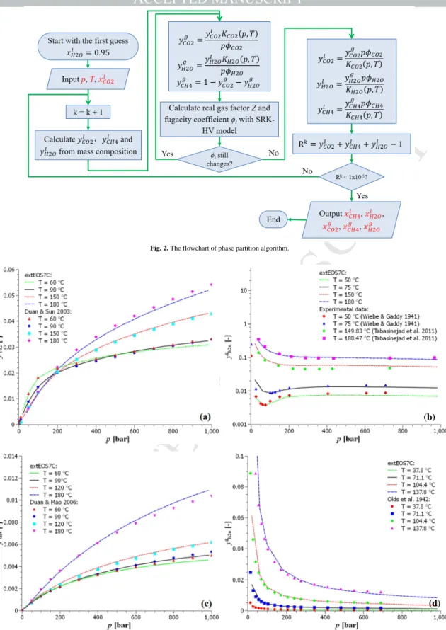
cannot be used directly. In such a case, the above algorithm is modified as follows (Fig. 2): Choosing the water mass fraction l2
H O
x as the variable (its initial value is assumed as 0.95, since the solubility of gas is small), the molar fraction of CO2, H2O and CH4 in the liquid phase can be calculated as
l l l / ( / ) i i i j j j x M y x M =
∑
(11)With the molar fraction of water and dissolved CO2, Eq. (9) is used to
calculate their molar fractions in the gas phase, while
4 g CH y is equal to 2 2 g g CO H O
1−y −y , so that the sum of gas molar fraction is equal to 1. Because the fugacity coefficient is dependent on the gas composition, several iterations are performed until constant values are achieved approximately. With the obtained gas compositions, the molar fractions of the dissolved gases are recalculated by using Eq. (9). These new values are then used to calculate the residual values, namely
l l
3
( ) i i 1 0
R x =
∑
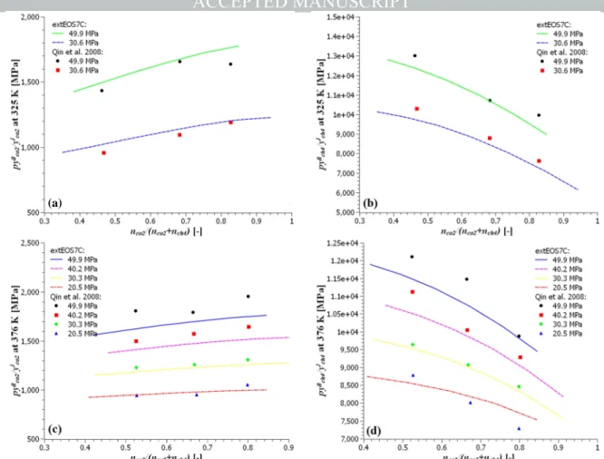
y − = (12) The above nonlinear equation is solved using Newton-Raphson iteration method. After that the molar fractions are converted to mass fractions for the mass transport simulation in TOUGH2MP.With the developed algorithm, the compositions of gas and aqueous phases can be obtained. The simulation results are shown in Fig. 3. The simulated results of gas solubility in aqueous phase for the pressure range of 0 – 1000 bar and temperature range of 60 °C – 180 °C are shown in Fig. 3a and c. They were compared with the results from Duan and Sun (2003) and Duan and Mao (2006), which have been validated by a large number of experimental data. For the CO2-H2O binary system, the calculated water molar fractions in gas
phase (Fig. 3b) were compared with the experimental data from Wiebe and Gaddy (1941) and Tabasinejad et al. (2011) (summarized in Li et al. (2015)). For the CH4-H2O binary system, the calculated water molar fractions in gas
phase (Fig. 3d) were compared with the experimental data from Olds et al. (1942). It can be seen that most of the data can be reproduced by the developed model in this study. Some misfit between the experimental data and simulation results may be due to the fact that the molar volumes of the components (Eq. (10)) are also dependent on pressure and temperature, but in this model only average values are adopted.
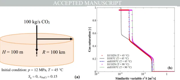
The mutual solubility of CO2 and CH4 in the CO2-CH4-H2O ternary system
is also simulated with the developed model. The results are shown in Fig. 4. The simulation results under various pressures in the range of 20.5 MPa and 49.9 MPa and temperatures (51.85 °C and 102.85 °C) were compared with the experimental results from Qin et al. (2008). In their work, the relationship between the apparent Henry’s law constant (defined as pyg/yl for each
component) and the ratio of CO2 and CH4 in the reaction cell was analyzed.
With the same gas partial pressure, the larger the Henry’s law constant is, the smaller the gas solubility in the aqueous phase will be. It can be seen that the CO2 solubility increases in the presence of CH4 for all the results, while the
CH4 solubility increases in the presence of CO2. This trend is consistent with
the experimental results. However, due to the limited number of experimental data points under each temperature, there are still discrepancies. Especially under high pressure conditions at 102.85 °C, the developed model overestimates the CO2 solubility and underestimates the CH4 solubility in the
aqueous phase. Further researches are required to address the reasons of this inaccuracy.
M
AN
US
CR
IP
T
AC
CE
PT
ED
Fig. 2. The flowchart of phase partition algorithm.
Fig. 3. The simulated phase partition without the dissolved NaCl: (a) calculated molar fractions of CO2 in liquid phase of the CO2-H2O system compared with the results from Duan and
Sun (2003); (b) calculated molar fractions of H2O in gas phase of the CO2-H2O system compared with the experimental data from Wiebe and Gaddy (1941), and Tabasinejad et al. (2011);
(c) calculated molar fractions of CH4 in liquid phase of the CH4-H2O system compared with the results from Duan and Mao (2006); (d) calculated molar fractions of H2O in gas phase of
the CH4-H2O system compared with the experimental data from Olds et al. (1942).
(b)
M
AN
US
CR
IP
T
AC
CE
PT
ED
Fig. 4. The simulated phase partition of the CO2-CH4-H2O system without the dissolved NaCl compared with the experimental data from Qin et al. (2008): (a) the simulated and measured
apparent Henry’s constants for CO2 at 51.85 °C; (b) the simulated and measured apparent Henry’s constants for CH4 at 51.85 °C; (c) the simulated and measured apparent Henry’s
constants for CO2 at 102.85 °C; (d) the simulated and measured apparent Henry’s constants for CH4 at 102.85 °C.
2
CO
n and 4
CH
n stand for the total molar fractions of each component in the whole system.
2.2. Consideration of dissolved salt in brine
By adding the activity coefficient in the phase partition calculation (Eq. (9)), the influences of dissolved salt on the gas solubility can be considered. In this study, the activity coefficient for CO2 is calculated according to Duan and
Sun (2003) using the following equation:
2 2 2
CO CO Na Na CO Nal Cl Na Cl
lnγ =2λ − m +ς − − m m (13) whereλCO2−NaandςCO2−Nal Cl− are the second- and third-order interaction
parameters for CO2 dissolved in water, respectively. These parameters are
calculated by 2 3 5 1 2 4 6 ( , ) 630 c c par p T c c T c T c p T T = + + + + − + + 2 8 9 10 7 ln 630 (630 )2 11 ln c p c p c p c p T c T p T T T + + + + − − (14)
where par is the interaction parameters, and ci (i = 1, 2 …, 11) is the fitting parameter and listed in Table A2 in Appendix A. The activity coefficient for CH4 is calculated according to Duan and Mao (2006) using the following
equation: 4 4 4 CH CH Na Na CH Nal Cl Na Cl lnγ =2λ − m +ς − − m m (15) where 4 CH Na
λ − andςCH4−Nal Cl− are the second- and third-order interaction
parameters for CH4 dissolved in water, respectively. These parameters are
calculated by 2 3 5 1 2 4 2 ( , ) c c par p T c c T c T T T = + + + + +
2 8 9 6 7 2 10 c p c p c p c pT c p T T T + + + + (16)
With the developed algorithm, the phase compositions under various pressures (0 – 1000 bar), temperatures (60 °C – 150 °C) and salinities (0 mol/kg, 2 mol/kg, 4 mol/kg) were simulated. Fig. 5a and c shows the CO2 and
CH4 molar fractions in gas phase of a binary system, respectively. The
simulation results were also compared with the results from Duan and Sun (2003) and Duan and Mao (2006). They match well with each other. Fig. 5b shows the corresponding H2O molar fractions in gas phase of the CH4-H2O
mixture under various conditions, while Fig. 5d shows the H2O molar
fractions in gas phase of the CO2-H2O mixture. 2.3. Thermodynamic properties of brine
The brine properties are dependent on pressure, temperature, salinity, etc. In this study, the brine viscosity is calculated with the model from Mao and Duan (2009), which is valid up to 623 K and 1000 bar. In this model, a simpler formulation for the viscosity of liquid water is developed without the loss of accuracy. The calculation is much faster than the complicated IAPWS formulation from Huber et al. (2009).
Similar to that in ECO2N module, the brine density is calculated as
2 4 2 4 2 4 l l l l CO CH CO CH mix b CO CH 1 1 x x x x ρ ρ ρ ρ − − = + + (17) where ρb is the brine density (kg/m3) without dissolved gas calculated
according to Haas (1976) and Andersen et al. (1992), and ρCO2andρCH4are the densities (kg/m3) of dissolved gases calculated according to the respective molar mass and the partial molar volume. The partial molar volume of CO2 is
obtained from Garcia (2001), while the partial molar volume of CH4 is
calculated according to Duan and Mao (2006). It should be emphasized that
t h e
M
AN
US
CR
IP
T
AC
CE
PT
ED
Fig. 5. The simulated phase partition with different NaCl molalities: (a) calculated CO2 molar fraction in liquid phase of the CO2-H2O system compared with the results from Duan and
Sun (2003); (b) calculated H2O molar fraction in gas phase of the CO2-H2O system; (c) calculated CH4 molar fraction in liquid phase of the CH4-H2O system compared with the results
from Duan and Mao (2006); (d) calculated H2O molar fraction in gas phase of the CH4-H2O system.
brine density will increase with the dissolution of CO2 but decrease with the
dissolution of CH4. 2.4. Verification example
The extEOS7C module was implemented in TOUGH2MP. The simulator is verified by two examples. The first one is the radial flow from a CO2 injection
well, which is taken from Pruess (2005). The second one is the Taggart’s problem described in Taggart (2010) and Oldenburg et al. (2013).
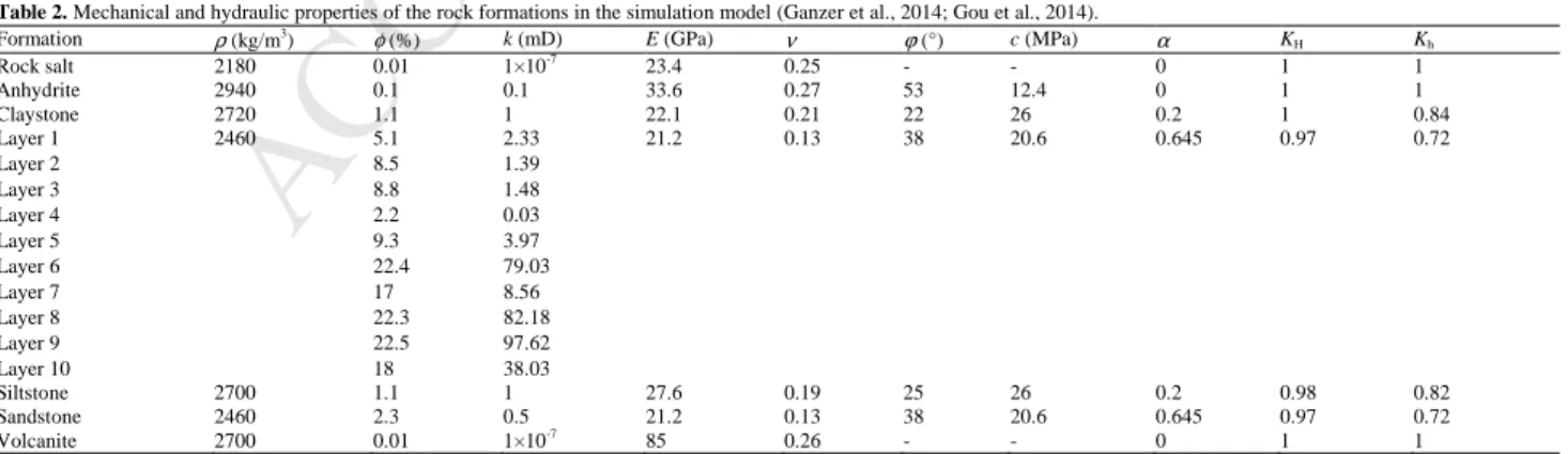
In the first example, CO2 is injected into a homogenous and isotropic saline
formation (Fig. 6a). The saline aquifer with a thickness of 100 m lies at the depth of 1200 m, and it has a porosity of 0.12 and permeability of 100 mD. The initial pressure of the aquifer is 12 MPa and the reservoir temperature is 45 °C. The salinity of the brine is 15%. CO2 is injected at a constant rate of
100 kg/s. A one-dimensional (1D) radial model of the aquifer is built with the internal mesh generation module of TOUGH2MP. The model has a radius of 100 km and is discretized into 435 grid cells. The upper and lower boundaries are impermeable, while the outer boundary in the radial direction has a very large volume to represent a constant reservoir condition (infinite-acting). The geomechanical effects are not considered in this example.
The simulated gas saturation is shown as functions of similarity variable ζ =
r2/t in Fig. 6b. Since there are time (t) and coordinate (r) in the similarity variable, the temporal evolution of gas saturation at r = 25.25 m is used for plotting. It can be seen that the dry-out simulated with EOS7C (ζ≈ 1×10⁻⁶ m2/s, t ≈ 20 yr) takes obvious longer time than those with ECO2N and
extEOS7C (ζ≈ 1×10⁻⁵ m2/s, t ≈ 2 yr), although the gas phase appears in the
grid cell at almost the same time. The reason is that the evaporation model adopted in EOS7C underestimates the water mass fraction in the gas phase. Fig. 6b shows also the simulation results from both of the codes under high temperature conditions, e.g. T = 90 °C. It can be seen that the gas exsolution occurred earlier than that under lower temperature conditions. The results from extEOS7C and ECO2N match well with each other, and thus this EOS module can be verified.
In the second example, a 1D model of 61 m × 0.3048 m × 0.3048 m (200 ft × 1 ft × 1ft) was set up to study the extraction of dissolved CH4 from a
saturated formation through CO2 injection (Fig. 7a). The formation has a
porosity of 0.25 and permeability of 1 D. The injection occurs at the left boundary, while the right boundary has a constant pressure. The injection rate is circa 0.159 m3/d (1 bbl/d) at the reservoir condition. More details can be found in Oldenburg et al. (2013). This problem was simulated with the developed extEOS7C module. The simulation results at t = 3 d are shown in Fig. 7b-d. Fig. 7b shows the distribution of the pressure and gas saturation along the model. It can be seen that the pressure and gas saturation near the injection well have small mismatches. This is due to the fact that the CO2
density predicted by SRK model is lower than that predicted by Peng-Robinson EOS. Fig. 7c shows the CO2 and CH4 mass fractions in the gas
phase, while Fig. 7d shows their mass fractions in the liquid phase. The gaseous CH4 bank ahead of the CO2 plume can be seen clearly, and the results
from extEOS7C match well with the results from Oldenburg et al. (2013).
(b)
M
AN
US
CR
IP
T
AC
CE
PT
ED
Fig. 6. (a) Schematic chart of the verification example 1 (Pruess, 2005); (b) Comparison of the simulated gas saturation as a function of similarity variable.
Fig. 7. (a) Schematic chart of the verification example 2 (Taggart, 2010; Oldenburg et al., 2013); (b) Comparison of gas pressure and saturation distributions; (c) Comparison of CO2 and
CH4 mass fractions in gas phase; (d) Comparison of CO2 and CH4 mass fractions in liquid phase along the model.
3. Application example
With the newly developed extEOS7C module, the CO2-EGR process was
investigated with numerical simulations. In this study, a simplified 3D model was built based on the geological structure and stratigraphy of a gas reservoir in the North German Basin. The main gas reservoir includes 10 sandstone layers and 9 siltstone layers of the upper Permian Rotliegend formation. It lies at the depth of about 3500 m and is covered by Zechstein salt formations. The gas reservoir is occupied by gas and connate water with the initial reservoir pressure of 42 MPa and temperature of about 125 °C. After many years’ production, the reservoir pressure dropped to 5 MPa. The average reservoir
porosity and permeability are 21% and 11 mD, respectively. More details can be found in Singh et al. (2012), Ganzer et al. (2014) and Gou et al. (2014).
The simulation model in this study is a simplified 1/4 model with a dimension of 2200 m × 1000 m × 1000 m (Fig. 8). It is discretized into 50,600 rectangular elements. The 1/4 model contains an injection well and a production well. They are 1800 m away from each other. The elements near the injection and production wells are fine discretized. The model includes not only the sandstone and siltstone layers but also 550 m caprock, i.e. rock salt and anhydrite, and 245 m basement rocks.
Initial condition: p = 12 MPa, T = 45 °C
S
g= 0, x
NaCl= 0.15
(b)
(a)
M
AN
US
CR
IP
T
AC
CE
PT
ED
Fig. 8. Simplified 3D 1/4 simulation model.
The rock properties of each reservoir formation are different (Table 2). The porosity and permeability of the formation rocks were measured in the laboratory with core plugs (Ganzer et al., 2014). For hydraulic simulation in this study, the average porosity and permeability for each of the rock formation layers were adopted. The layers 6–10 have larger porosity and thickness, so CO2 injection and gas production take place in these layers.
During the simulation, all boundaries were assumed to be closed. For the mechanical simulation, the properties were taken from Gou et al. (2014) (Table 2). The rock properties, including rock density, Young's modulus, Poisson's ratio and Biot’s coefficient, were determined with core samples retrieved in the North German Basin using RACOS@ (Rock Anisotropy
Characterization on Samples) (Braun et al., 1999). The strength parameters, including internal friction angle and cohesion, were determined with triaxial compression tests in the laboratory. The rock salt and volcanic basement rocks were assumed to be elastic materials, while other formations were described by the Mohr–Coulomb constitutive model. As the mechanical boundary conditions, four lateral boundaries and the bottom were fixed in the vertical direction, while vertical compression stress was applied to the top boundary. The initial stress was also measured with RACOS@ (Gou et al., 2014). The
determined ratios of horizontal effective stress to vertical effective stress for different rock formations (KH= ′σH/σ′v, Kh= ′σh/σ′v) are listed in Table 2. In this study, the minimum horizontal stress lies in the X-direction.
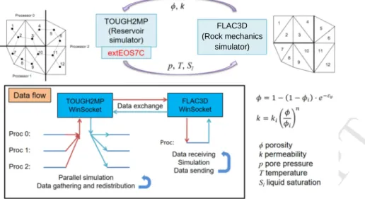
TOUGH2MP-FLAC3D was used to simulate the coupled THM process (Fig. 9). It was developed based on the coupling approach of TOUGH-FLAC
by Rutqvist and Tsang (2002) and Rutqvist et al. (2002). TOUGH2MP is the parallel version of the TOUGH2 code. In comparison to its serial version, TOUGH2MP can divide a simulation domain into many subdomains and distribute them to various cores on multi-CPU platforms. By solving the nonlinear systems of subdomains with several cores, the code performance is strongly improved. In the coupled simulator, data from two codes are exchanged in every time step through Windows Sockets. During each time step, TOUGH2MP will calculate the pore pressure, fluid composition, saturation and temperature of the model. These variables are then collected from each processor and transferred to FLAC3D for mechanical simulation. After the mechanical simulation, the new deformations and stresses will be transferred back to TOUGH2MP and distributed on the corresponding processors. These variables are then used to correct the hydraulic parameters for the next time step. The flowchart of the coupled THM simulator is shown in Fig. 9. In this study, we use the coupling model by Chin et al. (2010) and Cappa and Rutqvist (2011). In this model, the permeability change due to the deformation is related to the volumetric strain εv as
v i 1 (1 )eε φ= − −φ − (18) i i n k k φ φ = (19)
where φ and k are the porosity and permeability (m2) with deformation, respectively; φi and ki are the porosity and permeability (m2) without any
deformation, respectively; and n is a material parameter (here n=15).
Table 2. Mechanical and hydraulic properties of the rock formations in the simulation model (Ganzer et al., 2014; Gou et al., 2014).
Formation ρ (kg/m3 ) φ (%) k (mD) E (GPa) ν ϕ (°) c (MPa) α KH Kh Rock salt 2180 0.01 1×10⁻⁷ 23.4 0.25 - - 0 1 1 Anhydrite 2940 0.1 0.1 33.6 0.27 53 12.4 0 1 1 Claystone 2720 1.1 1 22.1 0.21 22 26 0.2 1 0.84 Layer 1 2460 5.1 2.33 21.2 0.13 38 20.6 0.645 0.97 0.72 Layer 2 8.5 1.39 Layer 3 8.8 1.48 Layer 4 2.2 0.03 Layer 5 9.3 3.97 Layer 6 22.4 79.03 Layer 7 17 8.56 Layer 8 22.3 82.18 Layer 9 22.5 97.62 Layer 10 18 38.03 Siltstone 2700 1.1 1 27.6 0.19 25 26 0.2 0.98 0.82 Sandstone 2460 2.3 0.5 21.2 0.13 38 20.6 0.645 0.97 0.72 Volcanite 2700 0.01 1×10⁻⁷ 85 0.26 - - 0 1 1
M
AN
US
CR
IP
T
AC
CE
PT
ED
Fig. 9. The flowchart of coupled THM simulator TOUGH2MP-FLAC3D with extEOS7C module.
In this study, the CO2-EGR and storage process under various pressures,
temperatures and salinities were investigated. As the baseline case, a geothermal gradient of 30 °C/km was adopted and the temperature on the land surface was assumed as 20 °C. Based on these values, the initial temperature of the reservoir (T0) was about 125 °C. The salinity of formation water was
not considered (xs = 0). CO2 was injected into layers 6–10 at a total injection
rate of 50,000 t/yr in the 1/4 model, i.e. 200,000 t/yr for the whole model during 5 years. The injection started either before primary production with an initial pore pressure p0≈ 42 MPa or at depleted state with an initial pore
pressure p0≈ 5 MPa. For these cases, the pore pressure at the depth of −3440
m (injection section) was assumed as 42 MPa, while 5 MPa for the depleted case. The pore pressures at the other grid cells were calculated with a gradient of 1743 Pa/m, while 250 Pa/m for the depleted case, depending on the gas density. The gas production rate was 50,000 sm3/d in the 1/4 model, i.e. 200,000 sm3/d for the whole model. The injection and production rates for each layer were averaged from the total rate according to the thickness. After that simulations were run with the initial salinity of 28% (almost saturated brine) to address the effects of dissolved salt. At last the initial reservoir temperature was also varied by ±20 °C to study the influences of temperature.
4. Simulation results and discussion
Fig. 10 shows the simulation results for the initial reservoir pressure of 5 MPa at depleted state with CO2 injection and gas production. Under this initial
condition, CO2 was injected at a super-heated gas state. The gas saturation
does not change obviously because most of the formation water is connate water. Fig. 10a shows the distribution of CO2 mass fraction in the gas phase at
the end of 5 years’ injection and production. It can be seen that CO2 transport
in each layer differs because of the different flow capacities. CO2 was
transferred further in the injection layers with relatively higher permeability (layers 6–10). Especially in the layer 9, CO2 breakthrough occurred already at
the end of the 5th year. Although the mass fraction of CO2 in the gas phase in
the production well was still low, the produced gas started to degrade (Fig. 10d). Because the density of CO2 (100 kg/m3) is larger than that of CH4 (25
kg/m3), the injected gases moved also downward to the lower sandstone layers and reached the volcanic basement formation. It did not penetrate into the
ultra-low permeable caprock (rock salt). Fig. 10b shows the pressure distribution in the whole model. With such injection and production rates, the pore pressure change in the reservoir was small. The maximum pore pressure change occurred in the layer 7. In this layer, the pore pressure at the injection zone was increased by 1.6 MPa, while that in the production zone was decreased by 0.5 MPa. The pore pressure increase below the layer 10 (bottom of the main reservoir) was about 0.7 MPa, which is comparable to that in the upper part of the main reservoir. Fig. 10c shows the vertical displacement of the model. The uplift occurred mainly near the injection well, while the nearby region of the production well had almost no vertical movement. The maximum uplift of 3.6 mm occurred at the bottom of the caprock (rock salt), since the pore pressure was transferred into the upper part of the reservoir but almost not into the caprock. This is consistent with the simulation results with a 2D model in Hou et al. (2012). Fig. 10d shows the CO2 breakthrough curves
at different positions along the profile through injection and production zones in the layer 9. It can be seen that CO2 in the gas phase reached 500 m after
about 0.4 year and 1000 m after about 1.8 years.
Fig. 11 shows the simulation results for the initial reservoir pressure of 5 MPa with only CO2 storage. It can be clearly seen that the CO2 transport
process was almost not affected by the gas production with the rate of 200,000 sm3/d in this case (Fig. 11a). However, the gas production did have influences on the reservoir pressure. The maximum pore pressure was 7.09 MPa, which is a little higher than that with production. The maximum and average reservoir pressure changes were 2 MPa and 0.75 MPa, respectively. Fig. 11b shows the distribution of vertical displacement along the section across the injection well (Y = 0). The maximum vertical displacement of 6.9 mm occurred at the bottom of caprock and was twice the vertical displacement with gas production. The vertical displacement decreased by 2 mm along the X-axis from the injection zone to the far field. Fig. 11c shows the stress and pore pressure changes along the vertical line through the injection zone. Both the pore pressure and stress changes were very low. Similar to the case of gas production, the pore pressure increase below the bottom of the main reservoir was comparable to that in the upper part of the main reservoir. According to Rutqvist (2012), the increase of horizontal stresses is correlated with the pore pressure change under elastic conditions. The simulation results in this study c o n f i r m e d t h i s
FLAC3D (Rock mechanics
M
AN
US
CR
IP
T
AC
CE
PT
ED
Fig. 10. (a) Contour of CO2 mass fraction in the gas phase; (b) Contour of pore pressure; (c) Contour of vertical displacement at the end of 5 years’ CO2 injection and CH4 production (p0 ≈
5 MPa, T0 ≈ 125 °C, xs = 0); (d) Breakthrough curves of different locations along the line through injection and production zones in the layer 9.
Fig. 11. (a) Contour of CO2 mass fraction in the gas phase; (b) Vertical displacement along the section across the injection well (Y = 0); (c) Changes of total stress and pore pressure along
the vertical line through the injection zone (positive values mean the increase in compressive stress or pore pressure) at the end of 5 years’ CO2 injection; (d) Stress path of caprock bottom
(rock salt) and injection zone of layer 7 (sandstone) (p0 ≈ 5 MPa, T0 ≈ 125 °C, xs = 0).
M
AN
US
CR
IP
T
AC
CE
PT
ED
relationship. Fig. 11d shows the stress path of the injection zone of layer 7 that had the highest pore pressure increase and the caprock bottom above it. It is clearly seen that the stress point of injection zone moved to the left after injection started. However, it was still far away from the rock strength and even the cohesionless rock strength, e.g. for possible micro-fractures in the rock. The stress state at the bottom of the caprock was not changed, so that its mechanical integrity can be guaranteed.
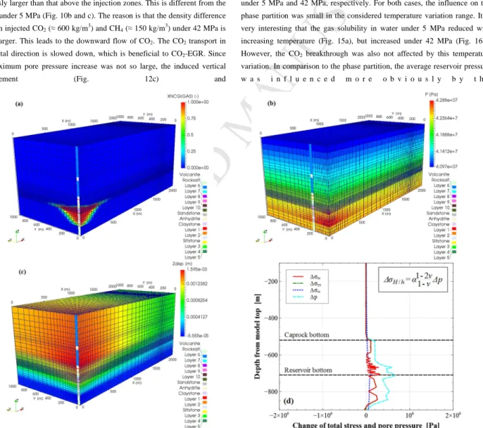
Fig. 12 shows the simulation results for the initial reservoir pressure of 42 MPa in the condition before the primary production with CO2 injection and
gas production. With this initial condition, CO2 was injected at a supercritical
state, at which the density and viscosity become much larger. This resulted in that CO2 stayed only in the nearby region of the injection well. Even in the
layer 7, CO2 reached about 800 m at the end of 5 years’ injection and
production (Fig. 12a). The pore pressure distribution is shown in Fig. 12b. The maximum pressure increase was only 0.6 MPa and occurred in the main reservoir area. This is due to the fact that the injected gas volume was lower, compared with the case with initial reservoir pressure of 5 MPa. The initial gas in place was still large, so that the influence of production was smaller. The pore pressure increase below layer 10 (main reservoir bottom) was obviously larger than that above the injection zones. This is different from the results under 5 MPa (Fig. 10b and c). The reason is that the density difference between injected CO2 (≈ 600 kg/m3) and CH4 (≈ 150 kg/m3) under 42 MPa is
much larger. This leads to the downward flow of CO2. The CO2 transport in
horizontal direction is slowed down, which is beneficial to CO2-EGR. Since
the maximum pore pressure increase was not so large, the induced vertical displacement (Fig. 12c) and
stress change were also relatively low (Fig. 12d).
In order to address the effects of dissolved salt, simulations were run with the initial salinity of 28% (almost saturated brine). Fig. 13a shows the comparison of the CO2 mass fraction along the profile through injection and
production zones in the layer 9 after 2 years’ CO2 injection and CH4
production. It can be seen that the CO2 mass fraction in gas phase was larger
but that in liquid phase was smaller, if there was salt dissolved in the formation water. The gas solubility was reduced because of the dissolved salt. However, CO2 breakthrough was almost not affected by the formation
salinity. Fig. 13b shows the development of average reservoir pressure for both cases. The pressure increase for the case with saturated brine (0.22 MPa) was slightly larger than that without salinity (0.2 MPa). Fig. 14 shows the results for the initial pressure of 42 MPa. Under that condition the CO2 mass
fraction in the gas phase was almost not affected, while that in the liquid phase showed the same tendency (Fig. 14a). The average reservoir pressure increase without and with dissolved salt was 0.14 MPa and 0.15 MPa, respectively (Fig. 14b). The difference was small.
In order to study the impacts of reservoir temperature, simulations were run with the temperature variations of ±20 °C. Figs. 15 and 16 show the results under 5 MPa and 42 MPa, respectively. For both cases, the influence on the phase partition was small in the considered temperature variation range. It is very interesting that the gas solubility in water under 5 MPa reduced with increasing temperature (Fig. 15a), but increased under 42 MPa (Fig. 16a). However, the CO2 breakthrough was also not affected by this temperature
variation. In comparison to the phase partition, the average reservoir pressure w a s i n f l u e n c e d m o r e o b v i o u s l y b y t h e
Fig. 12. (a) Contour of CO2 mass fraction in the gas phase; (b) Contour of pore pressure; (c) Contour of vertical displacement; (d) Stress change along the vertical line through the
M
AN
US
CR
IP
T
AC
CE
PT
ED
Fig. 13. (a) CO2 mass fraction along the line through injection and production zones in the layer 9 after 2 years’ CO2 injection and CH4 production; (b) Development of average reservoir
pressure with different initial salinities (p0 ≈ 5 MPa, T0 ≈ 125 °C, xs = 0 and 0.28).
Fig. 14. (a) CO2 mass fraction along the line through injection and production zones in the layer 9 at the end of 5 years’ CO2 injection and CH4 production; (b) Development of average
reservoir pressure with different initial salinities (p0 ≈ 42 MPa, T0 ≈ 125 °C, xs = 0 and 0.28).
Fig. 15. (a) CO2 mass fraction along the line through injection and production zone in the layer 9 after 2 years’ CO2 injection and CH4 production; (b) Development of average reservoir
pressure with temperature variations (p0 ≈ 5 MPa, T0 ≈ (125 ± 20) °C, xs = 0).
temperature variation. With the initial pressure of 5 MPa and initial temperatures of 105 °C, 125 °C and 150 °C, the respective pressure increases were 0.16 MPa, 0.2 MPa and 0.26 MPa (Fig. 15b). With the initial pressure of 42 MPa and initial temperatures of 105 °C, 125 °C and 150 °C, the respective pressure increases were 0.1 MPa, 0.14 MPa and 0.18 MPa (Fig. 16b). The difference was also larger than that induced by the salinity variation.
5. Conclusions
In this paper, the extEOS7C module was developed and implemented in the coupled THM simulator TOUGH2MP-FLAC3D. In comparison to the existing EOS7C module of TOUGH2MP, this module can calculate the phase partition of H2O-CO2-CH4-NaCl mixture accurately with consideration of
dissolved salt and real brine properties, especially at high pressure and temperature conditions (pressure up to 100 MPa and temperature up to 150 °C). The comparison between experimental and simulation results shows that most of the experimental data collected in this study can be reproduced with t h e d e v e l o p e d m o d u l e . T h e c o d e w a s u s e d i n
M
AN
US
CR
IP
T
AC
CE
PT
ED
Fig. 16. (a) CO2 mass fraction along the line through injection and production zone in the layer 9 at the end of 5 years’ CO2 injection and CH4 production; (b) Development of average
reservoir pressure with temperature variations (p0 ≈ 42 MPa, T0 ≈ 125 ± 20 °C, xs = 0).
the thermodynamic and coupled THM simulations of CO2-EGR with a
simplified 3D 1/4 model of a gas field in the North German Basin. The following conclusions can be drawn from the simulations:
(1) With the CO2 injection of 200,000 t/yr and gas production of 200,000
sm3/d, CO
2 breakthrough occurred in the case with the initial reservoir
pressure of 5 MPa but didn’t occur in the case of 42 MPa. This is mainly due to the increase of density and viscosity of injected CO2.
Under low reservoir pressure conditions, the pressure-driven horizontal transport is the dominant process; while under high reservoir pressure condition, the density-driven vertical flow is dominant during CO2
-EGR. CO2 breakthrough will increase the gas impurity and thus reduce
the efficiency of CO2-EGR. In order to slow down the breakthrough, it
is therefore suggested that CO2-EGR should be carried out before the
reservoir pressure drops below the critical pressure of CO2.
(2) For CO2-EGR, the maximum and average pressure changes under 42
MPa are smaller than those in the case with the initial reservoir pressure of 5 MPa. The reason is that the injected gas volume under 42 MPa is smaller than that under 5 MPa, and the initial gas in place is still large.
(3) The production rate of 200,000 sm3/d and its influences on CO 2
transport are still small in the considered cases. But these do reduce the average reservoir pressure (0.2 MPa), in comparison to the case with only CO2 injection with a pressure increase of 0.75 MPa.
(4) With a CO2 injection rate of 200,000 t/yr, the mechanical effect is very
small according to the simulation. Both reservoir and caprock behave elastically and there is no evidence of plastic deformations under the considered conditions. The largest uplift of 7 mm occurred at the bottom of the caprock above the injection zone in the case of only CO2
injection. Even in this case, the largest pore pressure and total stress change are 2 MPa and 1 MPa, respectively, and both of them occur in the reservoir formation (layer 7). Stress path analysis shows that the caprock has still the primary stress state and the caprock integrity is not affected.
(5) The influence of salinity on the CO2-EGR process is small under the
considered conditions. Although it changes the phase partition, especially the gas solubility in formation water, the CO2 breakthrough
is almost not affected.
(6) The temperature variations of ±20 °C have also small influences on the CO2-EGR process under the considered conditions. In comparison to
the effects of salinity, the phase partitions with temperature variations
of ±20 °C are almost not affected, but the average reservoir pressure change is relatively larger.
The extensions of EOS7C make it possible to simulate either CO2
sequestration in saline aquifer or CO2-EGR at high pressure and temperature
conditions. It can also be applied to the simulation of well fracturing treatment with energized gases. However, there are still limitations. For example, the pressure and temperature dependences of molar volume are not considered. There are still discrepancies during the phase partition calculation of CO2
-CH4-H2O ternary system at 102.85 °C under high pressure conditions. They
will be improved in the near future.
Conflict of interest
The authors wish to confirm that there are no known conflicts of interest associated with this publication and there has been no significant financial support for this work that could have influenced its outcome.
Acknowledgements
The work presented in this paper is funded by the National Natural Science Foundation of China (Grant No. NSFC51374147) and the German Society for Petroleum and Coal Science and Technology (Grant No. DGMK680-4).
References
Andersen G, Probst A, Murray L, Butler S. An accurate PVT model for geothermal fluids as represented by H2O-NaCl-CO2. In: Proceedings of the 17th Workshop on Geothermal
Reservoir Engineering. Stanford, USA: Stanford University; 1992. p. 239–48. Al-Hasami A, Ren S, Tohidi B. CO2 injection for enhanced gas recovery and geo-storage:
Reservoir simulation and economics. In: SPE EUROPEC/EAGE Annual Conference and Exhibition. Society of Petroleum Engineers; 2005. doi:10.2118/ 94129-MS. Austegard A, Solbraa E, De Koeijer G, Mølnvik MJ. Thermodynamic models for
calculating mutual solubilities in H2O–CO2–CH4 mixtures. Chemical Engineering
Research and Design 2006; 84(9): 781–94.
Braun R, Jahns E, Strommeyer D. Rock anisotropy characterization on samples (RACOS): Determination of rock mass structures and stress fields - Part 1: In situ stresses and rock anisotropy. Erdöl Erdgas Kohle 1999; 4: 191–7.
Cappa F, Rutqvist J. Modeling of coupled deformation and permeability evolution during fault reactivation induced by deep underground injection of CO2. International Journal
M
AN
US
CR
IP
T
AC
CE
PT
ED
Chin LY, Raghavan R, Thomas LK. Fully coupled geomechanics and fluid flow analysis of wells with stress-dependent permeability. SPE Journal 2000; 5(1): 32–45. Clemens T, Secklehner S, Mantatzis K, Jacobs B. Enhanced Gas Recovery - Challenges
shown at the example of three gas fields. In: SPE EUROPEC/EAGE Annual
Conference and Exhibition. Society of Petroleum Engineers; 2010.
doi:10.2118/130151-MS.
Duan Z, Sun R. An improved model calculating CO2 solubility in pure water and aqueous
NaCl solutions from 273 to 533 K and from 0 to 2000 bar. Chemical Geology, 2003; 193(3-4): 257–71.
Duan Z, Mao S. A thermodynamic model for calculating methane solubility, density and gas phase composition of methane-bearing aqueous fluids from 273 to 523 K and from 1 to 2000 bar. Geochimica et Cosmochimica Acta 2006; 70(13): 3369–86.
Eshkalak MO, Al-Shalabi EW, Sanaei A, Aybar U, Sepehrnoori K. Simulation study on the CO2-driven enhanced gas recovery with sequestration versus the re-fracturing
treatment of horizontal wells in the U.S. unconventional shale reservoirs. Journal of Natural Gas Science and Engineering, 2014; 21: 1015–24.
Ganzer L, Reitenbach V, Pudlo D, Albrecht D, Singhe AT, Awemo KN, Wienand J, Gaupp R. Experimental and numerical investigations on CO2 injection and enhanced
gas recovery effects in Altmark gas field (Central Germany). Acta Geotechnica, 2014; 9(1):39–47.
Garcia JE. Density of aqueous solutions of CO2. Report LBNL-49023. Berkeley, USA:
Lawrence Berkeley National Laboratory; 2001.
Gou Y, Hou Z, Liu H, Zhou L, Were P. Numerical simulation of carbon dioxide injection for enhanced gas recovery (CO2-EGR) in Altmark natural gas field. Acta Geotechnica,
2014; 9(1): 49–58.
Haas JL. Physical properties of the coexisting phases and thermochemical properties of the H2O component in boiling NaCl solutions. Washington, D.C.: US Geological
Survey Bulletin; 1976.
Honari A, Hughes TJ, Fridjonsson EO, Johns ML, May EF. Dispersion of supercritical CO2 and CH4 in consolidated porous media for enhanced gas recovery simulations.
International Journal of Greenhouse Gas Control 2013; 19: 234–42.
Hou Z, Gou Y, Taron J, Gorke UJ, Kolditz O. Thermo-hydro-mechanical modeling of carbon dioxide injection for enhanced gas-recovery (CO2-EGR): a benchmarking study for
code comparison. Environmental Earth Sciences 2012; 67(2): 549–61.
Hou Z, Xie H, Zhou H, Were P, Kolditz O. Unconventional gas resources in China. Environmental Earth Sciences 2015; 73(10): 5785–9.
Huber ML, Perkins RA, Laesecke A, Friend DG, Sengers JV, Assael MJ, Metaxa IN, Vogel E, Mareš R, Miyagawa K. New international formulation for the viscosity of H2O. Journal of Physical and Chemical Reference Data 2009; 38(2): 101–25.
Hughes TJ, Honari A, Graham BF, Chauhan AS, Johns ML, May EF. CO2 sequestration
for enhanced gas recovery: New measurements of supercritical CO2–CH4 dispersion in
porous media and a review of recent research. International Journal of Greenhouse Gas Control 2012; 9: 457–68.
Hussen C, Amin R, Madden G, Evans B. Reservoir simulation for enhanced gas recovery: An economic evaluation. Journal of Natural Gas Science and Engineering, 2012; 5: 42– 50.
International Association for the Properties of Water and Steam (IAPWS). Guideline on the Henry’s constant and vapor-liquid distribution constant for gases in H2O and D2O at
high temperatures. IAPWS; 2004.
Jikich SA, Smith DH, Sams WN, Bromhal GS. Enhanced gas recovery (EGR) with carbon dioxide sequestration: A simulation study of effects of injection strategy and operational parameters. In: SPE Eastern Regional Meeting.Society of Petroleum Engineers; 2003. doi:10.2118/84813-MS.
Kalantari-Dahaghi A. Numerical simulation and modeling of enhanced gas recovery and CO2 sequestration in shale gas reservoirs: A feasibility study. In: SPE International
Conference on CO2 Capture, Storage, and Utilization. Society of Petroleum Engineers;
2010. doi:10.2118/139701-MS.
Kalra S, Wu X. CO2 injection for enhanced gas recovery. In: SPE Western North
American and Rocky Mountain Joint Meeting. Society of Petroleum Engineers; 2014. doi:10.2118/169578-MS.
Kolditz O, Xie H, Hou Z, Were P, Zhou H. Subsurface energy systems in China: production, storage and conversion. Environmental Earth Sciences 2015; 73(11): 6727– 32.
Kühn M, Tesmer M, Pilz P, Meyer R, Reinicke K, Förster A, Kolditz O, Schäfer D, CLEAN Partners. CLEAN: project overview on CO2 large-scale enhanced gas recovery
in the Altmark natural gas field (Germany). Environmental Earth Sciences 2012; 67(2): 311–21.
Li J, Wei L, Li X. An improved cubic model for the mutual solubilities of CO2–CH4–H2S–
brine systems to high temperature, pressure and salinity. Applied Geochemistry 2015; 54: 1–12.
Liu H, Hou Z, Were P, Sun X, Gou Y. Numerical studies on CO2 injection-brine
extraction process in a low-medium temperature reservoir system. Environmental Earth Sciences 2015; 73: 6839–54.
Mao S, Duan Z. The viscosity of aqueous alkali-chloride Solutions up to 623 K, 1000 bar, and high ionic strength. International Journal of Thermophysics 2009; 30(5): 1510–23. Oldenburg CM, Pruess K, Benson SM. Process modeling of CO2 injection into natural gas
reservoirs for carbon sequestration and enhanced gas recovery. Energy & Fuels 2001; 15(2): 726–30.
Oldenburg, CM, Benson SM. CO2 injection for enhanced gas production and carbon
sequestration. In: SPE International Petroleum Conference and Exhibition in Mexico. Society of Petroleum Engineers; 2002. doi:10.2118/ 74367-MS.
Oldenburg CM, Moridis GJ, Spycher N, Pruess K. EOS7C Version 1.0: TOUGH2 module for carbon dioxide or nitrogen in natural gas (methane) reservoirs. Report LBNL-56589. Berkeley, USA: Lawrence Berkeley National Laboratory; 2004.
Oldenburg CM, Stevens SH, Benson SM. Economic feasibility of carbon sequestration with enhanced gas recovery (CSEGR). Energy 2004; 29(9–10): 1413–22.
Oldenburg CM, Doughty C, Spycher N. The role of CO2 in CH4 exsolution from deep
brine: Implications for geologic carbon sequestration. Greenhouse Gases: Science and Technology 2013; 3(5): 359–77.
Olds RH, Sage BH, Lacey WN. Phase equilibria in hydrocarbon systems. Composition of the dew-point gas of the methane-water system. Industrial & Engineering Chemistry 1942; 34(10): 1223–7.
Polak S, Grimstad AA. Reservoir simulation study of CO2 storage and CO2-EGR in the
Atzbach–Schwanenstadt gas field in Austria. Energy Procedia 2009; 1(1): 2961–8. Pooladi-Darvish M, Hong H, Theys SOP, Stocker R, Bachu S, Dashtgard S. CO2 injection
for enhanced gas recovery and geological storage of CO2 in the Long Coulee Glauconite
F Pool, Alberta. In: SPE Annual Technical Conference and Exhibition. Society of Petroleum Engineers; 2008. doi:10.2118/115789-MS.
Prausnitz JM, Lichtenthaler RN, Azevedo EGD. Molecular thermodynamics of fluid-phase equilibria. 3rd Edition. Prentice-Hall; 1999.
Pruess K. ECO2N: A TOUGH2 fluid property module for mixtures of water, NaCl, and CO2. Report LBNL-57952. Lawrence Berkeley National Laboratory, University of
California; 2005.
Pruess K, Spycher N. ECO2N – A fluid property module for the TOUGH2 code for studies of CO2 storage in saline aquifers. Energy Conversion and Management 2007;
48(6): 1761–7.
Qin J, Rosenbauer RJ, Duan Z. Experimental measurements of vapor-liquid equilibria of the H2O + CO2 + CH4 ternary system. Journal of Chemical & Engineering Data 2008;
53(6): 1246–9.
Reid RC, Prausnitz JM, Poling BE. The properties of gases and liquids. 4th Edition. New York: McGraw Hill Book Co.;1987.
Rutqvist J, Tsang CF. A study of caprock hydromechanical changes associated with CO2
injection into a brine formation. Environmental Geology 2002; 42(2): 296–305. Rutqvist J, Wu YS, Tsang CF, Bodvarsson G. A modeling approach for analysis of
coupled multiphase fluid flow, heat transfer, and deformation in fractured porous rock. International Journal of Rock Mechanics & Mining Sciences 2002; 39(4): 429–42.