Characterization of the ionospheric small-scale activity

IRM/GALOCAD/OUT220-1 OUT220-1 Version: 3 Contract ref: GJU/06/2423/CTR/GALOCAD Written by: R. Warnant, G. Wautelet, J. Spits, S. Lejeune Verified by: R. Warnant

GALOCAD

Development of a Galileo Local Component for the nowcasting

and forecasting of atmospheric disturbances affecting the

integrity of high precision Galileo applications.

WP 220 Technical Report:

“Characterization of the ionospheric Small-scale activity”

LIST OF ABBREVIATIONS

GI/BAS Geophysical Institute of the Bulgarian Academy of Sciences GNSS Global Navigation Satellite System

GPS Global Positioning System IMF Interplanetary Magnetic Field Kd K index for Dourbes (Belgium) NLS Noise-like structures

NWP Numerical Weather Prediction models RINEX Receiver Independent Exchange format RMI Royal Meteorological Institute ROB Royal Observatory of Belgium RoTEC Rate of TEC (TEC time derivative) RTK Real Time Kinematics

TEC Total Electron Content TECU TEC Unit

TID Travelling Ionospheric Disturbance

WP Work Package

TABLE OF CONTENT

List of abbreviations………2

Table of Content………..…3

1. Introduction………...………...4

2. Detection of ionospheric small-scale disturbances………..…4

2.1 Methodology………4

2.2 Type of structures observed in Europe at mid-latitudes………..8

3. Influence of cycle slips….………...9

3.1 Introduction………..9

3.2 Original method……….10

3.3 New method………...12

3.4 Conclusions………16

4. Small-scale disturbance climatology……….…16

4.1 Number of events – probability of occurrence………..16

4.2 Amplitude of TEC time derivative………23

4.3 Validation of the analysis………..………26

5. Gradients in space due to small-scale disturbances………..….32

5.1 The Belgian Active Geodetic Network………..32

5.2 Selection of days: case study……….33

5.3 Gradient detection using double differences: methodology……….….40

5.4 Quantitative analysis of ionospheric residual effects………43

5.5 Influence of baseline length and baseline orientation …..….………....48

5.6 Determination of “ionospheric disturbed conditions”………...52

6. Conclusions………...54

1. INTRODUCTION

The effect of the ionosphere on GNSS signals mainly depends on the Total Electron Content or TEC. The Total Electron Content is the integral of the ionosphere electron concentration on the receiver-to-satellite path. GNSS differential applications are based on the assumption that the measurements made by the reference station and by the mobile user are affected in the same way by the different error sources, in particular by the ionospheric effects. Therefore, these applications will not be affected by the absolute TEC but by gradients in TEC between the reference station and the user.

Small-scale structures in the ionosphere are the origin of gradients in TEC which can degrade the accuracy of differential applications even on distances of a few km. Such events could pose a threat for high accuracy GNSS applications. In this report, we characterize the different small-scale disturbances which can be encountered in a mid-latitude European station (Brussels, Belgium).

GNSS carrier phase measurements can be used to monitor local TEC variability. At any location, several GPS satellites can simultaneously be observed at different azimuths and elevations. Every satellite-to-receiver path allows to “scan” the ionosphere in a particular direction. The more satellites are simultaneously observed, the “denser” the information on the ionosphere is. In particular, small-scale ionospheric structures can be detected by monitoring TEC high frequency changes at a single station. Wanninger (1992) and Wanninger (1994) has developed a method allowing to monitor ionospheric irregularities based on a combination of GPS dual frequency phase measurements. In particular, this method was applied to scintillation monitoring in Brazil. Warnant (1996, 1998 and 2000) further developed the method for conducting “climatological” studies on small-scale ionospheric activity at the mid-latitude station in Brussels, Belgium.

2. DETECTION OF IONOSPHERIC SMALL-SCALE DISTURBANCES

2.1.

Methodology

As already mentioned, TEC variability can be monitored using GNSS measurements (Warnant et al., 2000).

The simplified mathematical model of phase measurements made by receiver A on satellite i, i_,

A k

ϕ (in cycles) can be written as follows (Seeber (2003); Leick (2004)):

i_, k

(

(

)

)

i A

D

, i

, the geometric distance between receiver A and satellite i ; A k

I , the ionospheric error (m) on carrier k; i

A

T , the tropospheric error (m);

A t Δ i t Δ , i

, the receiver clock error (the synchronisation error of the receiver time scale with respect to GPS time scale) ;

, the satellite clock synchronisation error (the synchronisation error of the satellite time scale with respect to GPS time scale) ;

A k N

, i

, the phase ambiguity on carrier k (integer number) ; A k

M , multipath effect on carrier k ; ,

i A k

ε , noise on carrier k ; k

f , the considered carrier frequency (L1 or L2).

If we neglect higher order terms (terms in 3 k

f − , 4

k

f − …), the ionospheric error i_,

A k I is given by: i_, 40.3 ₂Ai A k I k TEC f = (2.2) with : i A

TEC , the slant TEC from satellite i to receiver A (in electrons/m²).

The ionosphere TEC can be reconstructed from the so-called geometric free combination i_, A GF ϕ : 1 , , 1 2 i i L , i 2 A GF A L L f f ϕ =ϕ − i A L ϕ (2.3)

Based on equation (2.1) and equation (2.2), equation (2.3) can be rewritten in function of the slant TEC from receiver A to satellite i, TEC_A

16 , 552 10 , i i (Warnant et al, 2000): _0, i i_, i_, A GF A GF A GF ϕ ₌ − TEC_A+M_{A G} + ε F N + (2.4) Where i_, A GF N , i_, A GF M and i_, A GF

ε are respectively the geometric free ambiguity, multipath and noise: 1 , , 1 2 i i L , 2 i A GF A L A L L f N N N f = −

1 , ( , 1 i L i A GF A L A L f M M M c = − i_{, 2}) _(2.5) 1 , ( , 1 ) i L i A GF A L A L f c ε = ε −εi_{, 2}

This combination is called “geometric free” due to the fact that it does not contain geometric terms (i.e. satellite and receiver coordinates). Therefore, it cannot be used to compute the user position. In the absence of cycle slips, the real (non-integer) ambiguity

has to be solved for every satellite pass.

From Equation (2.4), it can be seen that, if we neglect multipath and noise, the geometry-free combination also allows monitoring the time variation of the TEC, e.g.

, i A G F N

( )

( )

(

( )

( )

)

(

)

and are 2 consecutive measurement epochs; , measured in TECU/min, is defined as:

1 k t ₋ TEC Δ k t

(

)

( )

( )

₍

₎

( )

It is important to stress that the computation of i

( )

Δ does not require the estimation of the real ambiguity, , as long as no cycle slip occurs. Equation (2.6) can be used to detect high frequency changes in the TEC due to irregular smaller-scale ionospheric phenomena.

The slant gradients computed by equation (2.6) are then verticalized by using a mapping function M and a simplified representation of the ionosphere. We assume that all the free

electrons in the ionosphere are contained in a thin spherical layer (the ionospheric shell).

The ionospheric shell is placed at an ionospheric height h, which is the height between

the thin shell and the ground surface; in our work, h is fixed at 400 km. The intersection

between the line-of-sight “satellite-station” and the ionospheric shell is called the

Ionospheric Pierce Point (IPP); so, to each measure of the gradients corresponds an IPP.

, i A G F N

Vertical gradients are computed as follows: i

( )

( )

(

)

if RT is the Earth radius (RT = 6371 km) and z is the zenithal angle of the satellite at the station. Angle zIPP is the zenithal angle of the satellite at the IPP.

The time derivation at different elevations when tracking a satellite introduces an artificial trend, not connected with the ionospheric variability, but due to the geometry of the satellite orbit. In order to remove the trend, we filter out the low frequency changes in the TEC by modeling vertical i

A

TEC

Δ i

using a low order polynomial. The residuals of this adjustment (i. e. vertical ΔTEC_A

R

- polynomial) contain the higher frequency terms and are called Rate of TEC (RoTEC).

Then, the standard deviation of the residuals, σ , is computed, separately for every satellite in view, on 15 minute periods. When σ_R > 0.08 TECU/min (on a 15 minute period), we decide that an “ionospheric event” is detected. In addition, an “ionospheric

intensity” is associated to every ionospheric event: the intensity of the event (the

amplitude of the associated TEC variations) is assessed based on a scale which ranges from 1 to 9 depending on the magnitude of σR. This quantity is a measure of amplitudes

of the small-scale irregularity structures, effectively degrading the accuracy of the GNSS differential positioning techniques.

The choice of the threshold value of 0.08 TECU/min comes from the fact that the multipath can also give rise to high frequency changes in the geometric-free combination. This site-dependent effect can reach several centimetres on phase measurements and has periods ranging from a few minutes to several hours depending on the distance separating the reflecting surface from the observing antenna (if this distance is shorter, the period is longer). The multipath effect being more frequent at low elevation, we have chosen an elevation mask of 20°. In the case of the Brussels permanent GPS station (on which the present study is based), a threshold value of 0.08 TECU/min is large enough to avoid interpreting multipath effects as ionospheric phenomena. This value should be valid for most of the GPS sites but should be applied with care in locations where the multipath is particularly important.

All the details concerning this technique (including the choice of the thresholds) are discussed in Warnant (1998) and Warnant et al. (2000).

2.2.

Types of structures observed in Europe at mid-latitudes

This methodology outlined in paragraph 2.1 has been applied to the continuous measurements collected at Brussels since April 1993.

Figure 2.1. Vertical TEC variability (rate of change in TECU/min) due to a TID observed at Brussels along the track of satellite 7 on DOY 340 in 2001.

From this study, it appears that TEC small-scale variability at mid-latitude (in Europe) is mainly related to two types of phenomena: Travelling Ionospheric Disturbances (TID’s) or “noise-like” variability. TID’s appear as waves in the electron density which is due to interactions between the ionosphere and the neutral atmosphere. They have wavelengths ranging from a few km to more than thousand km and periods of a few minutes up to 3 hours. Figure 2.1 shows the variability in vertical TEC (vertical TEC rate of change) due to a TID detected at Brussels on DOY 340 in 2001 (December 6 2001).

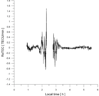
In mid-latitude stations, “noise-like” variability in TEC can also be observed. Such variability is mainly detected during geomagnetic storms. Figure 2.2 shows “noise-like” variability in vertical TEC due to a geomagnetic storm observed at Brussels on DOY 324 in 2002 (November 20 2002). The signature of these “noise-like” structures in TEC is very similar to the signature of scintillations which are variations in phase and amplitude of GNSS signals due to the presence of irregularities in the ionosphere electron concentration. Scintillations are only observed in the equatorial and in the polar regions but noise-like variability observed at mid-latitude during severe geomagnetic storms can also induce strong degradations in GNSS differential applications.

Warnant et al. (2007-1), Warnant et al. (2007-2) and Hernandez-Pajares et al. (2006) analyse in more details the ionospheric and geomagnetic conditions under which such variability appears mainly based on ionograms, GPS-TEC and geomagnetic measurements.

Figure 2.2. Noise-like variability in vertical TEC rate of change (in TECU/min) observed at Brussels during a geomagnetic storm on November 20 2002 along the

track of satellite 22.

3. INFLUENCE OF CYCLE SLIPS

3.1.

Introduction

In order to attain high precision in applications using GPS phase measurements, it is necessary to detect and remove cycle slips.

A cycle slip can be defined as a sudden jump (always an integer number of cycles) in the carrier phase observable. In fact, there are three main sources for cycle slips. Firstly (and most frequently), a cycle slip can be due to an obstruction of the satellite signal by some obstacles (trees, buildings…). Secondly, this can be due to a low signal-to-noise ratio caused by bad ionospheric conditions, multipath… Thirdly, a failure in the receiver software can cause a cycle slip.

All cycle slip detection processes are based on quantities derived from the observations, namely on linear combinations of the undifferenced carrier-phase (

φ

φ

Here, we use a cycle slip detection process in the preprocessing step of the “GPS-TEC” software (computation of the TEC and the TEC variability). It is then particularly important to adequately detect the cycle slips, in order to be sure that the ionospheric data are all there (no cycle detected instead of ionospheric variability) and correct (no cycle slip remaining).

3.2.

Original method

3.2.1. Principles

In the original “GPS-TEC” software, we use a cycle slip detection process based on a Kalman filter applied to two different linear combinations: the phase-range combination and the geometric-free phase combination.

In fact, we can form two mono-frequency phase-range combinations (RP1 and RP2) which can be written as follows:

1 1 1 1 P RP l ϕ = − 2 2 2 2 P RP l ϕ = −

with li the corresponding wavelength.

Because depending on pseudorange measurements, this combination has a relatively high noise level. Moreover, it depends on the ionospheric effects, which can lead to important epoch to epoch variations in the combination.

The dual-frequency geometric-free phase combination

φ

1 1 2 2 GF f f ϕ =ϕ − ϕ

with fi the corresponding frequency.

This combination is independent of the pseudorange measurements and is consequently a smoother quantity than the phase-range combination. However, it also depends on the ionospheric effects which can cause epoch to epoch changes.

3.2.2. Problems

As our objective is to characterize ionospheric activity, this original cycle slip detection process is not well adapted because it only uses ionospheric dependent data combinations. In case of high ionospheric activity, it is therefore really difficult to decide whether the changes in the data combination are due to cycle slips or to the ionospheric activity. As a consequence, there is a risk of interpreting abrupt changes in the considered combination as cycle slips when these changes are due in reality to ionospheric variability. In this context, even if the existing software was giving satisfying results in usual conditions, we noticed that during extreme ionospheric activity periods, this software was interpreting ionospheric variability as successive cycle slips and was removing long periods of data. This is a major problem due to the fact that the goal of our work is to detect and study periods with strong ionospheric activity.

Figure 3.1 and 3.2 illustrate the problem encountered with the existing cycle slip detection method; Figure 3.1 shows the data remaining after cycle slip detection with the old method: when the ionospheric variability increases above 1.5 TECU/min, the software interprets the data as successive cycle slips and removes these data. Figure 3.2 shows the same data but the threshold for cycle slip detection on the geometric free combination has been arbitrarily increased up to 10 cycles: the ionospheric variability is

not interpreted as cycle slip but in this way, there is an important risk to have remaining cycle slips in the data which could be interpreted as ionospheric variability. Therefore, we have developed and implemented a new method for cycle slip detection.

Figure 3.1. Ionospheric variability at BRUS – DOY 033/2002 – Satellite 8 Usual threshold for cycle slip detection

Figure 3.2 Ionospheric variability at BRUS – DOY 033/2002 – Satellite 8 Increased threshold for cycle slip detection

3.3.

New method

3.3.1. Principles

Therefore, in a second step, we have developed an improved cycle slip detection process based on the widelane phase minus narrowlane pseudorange combination

φ

(

)

As we can see, this combination consists of the widelane ambiguity , a residual code hardware delays term , a residual code multipath term and a residual code noise term .

1 2 12 N N N = − 12 M 12 d 12 s

For cycle slip detection purpose, the main advantage of this combination is its independence of the ionospheric effects.

However, the noise of this observable makes cycle slip detection unlikely1. That’s why we have to apply a running average filter (or low-pass filter) to this combination so that the residual terms average down to more or less constant values.

Let us present the main steps of the WL-NL cycle slip detection process applied:

1. First, we compute the recursive mean μ and the recursive standard deviation σ . The term recursive means that the mean and the standard deviation are computed and updated epoch by epoch.

2. Then, we calculate the relative confidence interval μ±4σ .

3. If the current value of the WL-NL combination is outside that interval, the data is declared to be an “outlier”.

4. If there are two consecutives outliers, we declare that a cycle slip has occurred and all the parameters are reinitialized: we start a new period and define a new ambiguity term.

5. If there is just one isolated outlier, it is removed from the data set but the parameters are not reinitialized.

Another advantage of this method is that it only uses statistical information from the data themselves, without the need of initializing parameters like in the Kalman filtering technique.

Figure 3.3 and 3.4 show the WL-NL combination in function of time in two different cases.

In figure 3.3 we can see that the WL-NL combination remains inside the confidence interval, except for two isolated points: two “outliers”. Those outliers are then removed from the data set. In figure 3.4, we can clearly identify a cycle slip, which is confirmed by the fact that the combination is outside the confidence interval during two consecutive epochs.

Figure 3.3 WL-NL combination at DENT – DOY 324-03 – Satellite 13

3.3.2. Analysis

In theory, one combination is sufficient for detecting cycle slips. But the characteristics of the WL-NL combination do not allow detecting a cycle slip whose value would be equal on

φ

φ

φ

In this context, instead of implementing a new combination, we will verify that the ionospheric variability values computed using the new method do not result from bad cycle slip detection and that they can be considered as real ionospheric variability. That point is particularly crucial in case of geomagnetic storm.

We have concentrated our analysis on the geomagnetic storm of DOY 324/03 (20/11/2003) for different stations, and precisely on t = 408480 s (GPS time) and t = 408510 s (for the satellites concerned). Contrary to the original method (figure 3.5), the new method does not detect cycle slips at BRUS at those epochs (and then does not delete data), which finally leads to very important ionospheric variability values (figure 3.6).

Figure 3.5. Ionospheric variability at BRUS – DOY 324/2003 – Satellite 2 Original cycle slip detection method used

Figure 3.6. Ionospheric variability at BRUS – DOY 324/2003 – Satellite 2 New cycle slip detection method used

We will try to prove that the ionospheric variability in figure 3.6 is real and not created by a cycle slip missed by the detection technique (i.e. equal on

φ

φ

First here are the “pro cycle slip” arguments:

1. We can show that the influence of a cycle slip on

φ

2. We can see that the phenomena appear at the same time in different stations (BRUS,DOUR,DENT,GILL…), which could be due to cycle slips caused by the ionospheric variability at the same time in the different stations.

Now let us develop the “ionospheric” arguments (with the corresponding numbering): 1. We can show that the influence of the ionospheric effects on

φ

* the value of the effect on RP1, which is the case here.

2. We can see that the phenomena appear at the same time in different stations (BRUS,DOUR,DENT,GILL…), which could be due to ionospheric variability (approximately the same conditions at the same time).

3. The RP1 and RP2 variations (at those epochs) are not exaggerated with regards to the possible ionospheric variability. Those changes are probably due to

ionospheric variability and not to cycle slips (which can cause random – and thus larger – slips).

4. The new method detects cycle slips at those critical epochs in BDN stations (like GILL,BATT…) which are equipped with LEICA GPS receivers and not in stations like BRUS,DENT… which are equipped with Ashtech GPS receivers. That point can be explained by the difference between the receivers at those stations. The receivers of the first group of stations (LEICA receivers) are more sensible to the ionospheric noise than those of the second group (ASHTECH receivers).

5. We can observe the same ionospheric variability structures for the different satellites and for the different stations.

6. When analyzing the IF (ionospheric free) and GF (geometric free) double-differenced phase measurements, there is no cycle slip detected for BRUS/DOUR or BRUS/DENT. Due to the ionospheric variability, the DD-GF combination is well noisy but there is no “jump” visible. For BRUS/GILL, we can however detect a cycle slip on both combinations (DD-IF and DD-GF), which confirms the fact that a real cycle slip occurs at GILL (it is detected by our new method) and not in BRUS for example.

All those “ionospheric” arguments show that the ionospheric variability of DOY 324/03 is real and not created by missed cycle slips. That confirms the validity of our developed technique.

3.4.

Conclusions

After analyzing the original cycle slip detection technique, we have concluded that it is not possible to improve it. In fact, we would not be able to determine the origin of the changes in the times series of the derived quantities (because of their dependence on the ionospheric effects): a cycle slip or the ionospheric variability? However, it is crucial because our objective is to use the data for TEC computing and analyzing.

For this reason, we have developed a new cycle slip detection technique based on running average filtering of the widelane-narrowlane combination. This combination has the advantage not to be dependent on the ionospheric effects and, even if it cannot detect equal cycle slip on

φ

φ

4. SMALL-SCALE DISTURBANCE “CLIMATOLOGY”

4.1.

Number of events – Probability of occurrence

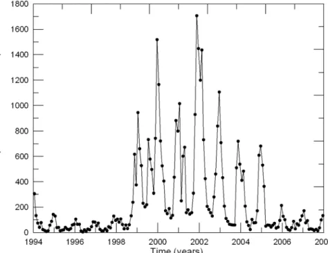
Figure 4.1 shows the number of “ionospheric events” (as defined above) detected per month at Brussels from January 1994 to December 2007. Most of these “events” are due to Travelling Ionospheric Disturbances (as already said, “noise-like” phenomena are mainly observed during geomagnetic storms).

Figure 4.1 Number of detected ionospheric events per month at Brussels from January 1994 to December 2007.

The analysis of figure 4.1 shows that:

- TID’s are frequently observed all the time (during all seasons and during all phases of the 11-year solar activity cycle).

- The number of detected events has an annual peak during winter time independently of solar activity but the peak is much sharper at solar maximum. - The number of TID’s strongly depends on the solar activity cycle: for example,

about 100 events were observed in December 1996, at solar minimum when more than 1500 events were detected in December 1999 and in November 2001 at solar maximum (the 2 peaks which are present in figure 4.1 correspond to the peaks of 2000 and 2002 observed in solar cycle 23).

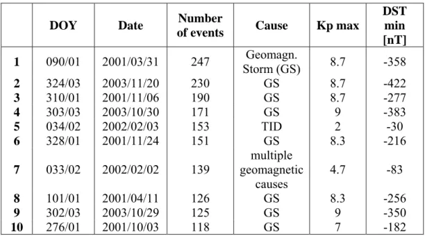
We can increase the temporal resolution from one month to one day in order to display the number of detected events per day. Figure 4.2 shows the evolution of the daily number of detected events from January 1994 to December 2006 (solar cycle 23). We can easily identify the most disturbed days (“worst cases”) in terms of ionospheric effects; moreover, table 1 contains the ten most disturbed days from 1994 to 2006 in terms of ionospheric events. The analysis of figure 4.2 and table 1 shows that the days that present a large number of events are mainly days where geomagnetic storms occurred. However, TID’s can induce strong ionospheric events and be at the origin of highly disturbed days. For example, DOY 034/02 is the fifth most disturbed day between 1994 and 2006 with 153 ionospheric events and an associated maximum TEC variability of 0.96 TECU/min.

Figure 4.2 Number of ionospheric events detected per day at Brussels from January 1994 to December 2006.

DOY Date Number

of events Cause Kp max

DST min [nT] Geomagn. Storm (GS) 1 090/01 2001/03/31 247 8.7 -358 2 324/03 2003/11/20 230 GS 8.7 -422 3 310/01 2001/11/06 190 GS 8.7 -277 4 303/03 2003/10/30 171 GS 9 -383 5 034/02 2002/02/03 153 TID 2 -30 6 328/01 2001/11/24 151 GS 8.3 -216 multiple geomagnetic causes 7 033/02 2002/02/02 139 4.7 -83 8 101/01 2001/04/11 126 GS 8.3 -256 9 302/03 2003/10/29 125 GS 9 -350 10 276/01 2001/10/03 118 GS 7 -182

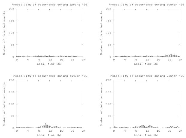
Ionospheric irregularities have also a dependence on season and local time. As it is shown in figure 4.3, ionospheric irregularities take mainly place during autumn and winter months. This result is verified for each phase of the solar cycle (minimum, maximum of activity).

Figure 4.3 Number of ionospheric events detected per month at Brussels for the year 2001 (solar maximum) and the year 2006 (solar minimum).

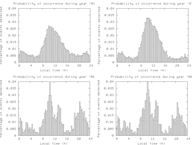
However, the occurrence of irregularities depends also on local time: in figure 4.4 we divide local time in periods of 15 minutes (in other words, there are 96 periods for 24 hours) and we show the total number of events which occurred in 2001 (left) and in 2006 (right) for each 15 minutes period. First, we'll analyze the year 2001 in order to characterize the mean behavior of the ionosphere during solar maximum. Then, the incidence of a low solar activity (2006) is analyzed.

Figure 4.4 Ionospheric event distribution at Brussels for the year 2001 (solar maximum) and the year 2006 (solar minimum) in function of local time.

4.1.1. High solar activity (2001)

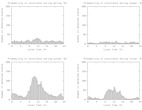
The analysis of the figure 4.4 (left) shows that most of irregularities occur around 10 A.M. There is also a secondary maximum observed during the night around 1 A.M. The periods characterized by a minimal ionospheric activity are located in the early morning (around 6 A.M.) and in the late afternoon (about 6 P.M.). This annual behavior can be divided into the four seasonal behaviors as we can see in figure 4.5. We can say that up to 50% of the annual number of ionospheric irregularities is produced during autumn; furthermore, let us note that winter behavior is quite similar to the autumn’s one.

In spring and summer, there are much less irregularities detected in comparison with autumn and winter and the behavior seems to be independent of local time.

Figure 4.5. Ionospheric events distribution in 2001 in function of the season and local time

4.1.2. Low solar activity (2006)

Figure 4.4 (right) shows three peaks: two around noon (main peak at 10 A.M. and secondary peak at 1 P.M.) and the third around 8 P.M. The minimal activity is still localized early in the morning and in the afternoon. Let us also note that the number of detected events is very low in comparison with the number of events detected during the

year 2001 at Solar maximum. As for the year 2001, let us decompose the annual distribution into the four seasonal behaviors; this is shown at the figure 4.6.

As for the year 2001, we can clearly observe that months of autumn and winter explain the major part of the annual distribution of the events in function of time. Nevertheless, the major part of the third peak comes from the summer days: there are nearly no irregularities during daytime in summer but the occurrence of such phenomena take place at sunset. This phenomenon was not visible for the year 2001.

Figure 4.6 Ionospheric events distribution in 2006 in function of the season and local time.

4.1.3. TID’s and noise-like structures

Ionospheric events presented in the previous statistics are mainly caused by TID’s and noise-like structures (NLS); we can try to separate these two components if we assume that NLS are due to disturbed geomagnetic conditions. We made the same statistics as previously (i.e. analysis of the ionospheric events distribution in function of local time) but only by using the days with no geomagnetic activity. In reality, we removed from our statistics the days that present a maximum daily value of Kp index equal or greater than 5; so we excluded all stormy days.

Figure 4.7 shows a similar graph than in figure 4.4 but when considering only days with Kpdaily max <5.

Figure 4.7 Ionospheric events distribution at Brussels for the year 2001 (solar maximum) and the year 2006 (solar minimum) in function of local time. All days

included present Kpdaily max <5.

Figure 4.8 Ionospheric events distribution at Brussels for year 2001 (top) and 2006 (bottom) if we include (left) or not (right) the days which present Kpdaily max >5.

For more readability, we chose to normalize the distribution by dividing each value (i.e. each value of detected events per 15min interval) by the total number of events detected during all the considered year. This leads to the figure 4.8 which shows that the shape of the distribution is similar if we include or not the days where geomagnetic storms occurred. In fact, stormy days induce an offset of the number of events detected (as seen in figure 4.4 and 4.7); this means that noise-like structures due to geomagnetic storms occur all the time, contrary to the TID distribution that shows a specific shape with a maximum around 10 A.M. Thus we can also affirm that most of ionospheric disturbances observed at Brussels are TID’s.

4.1.4. Conclusions

The number of ionospheric irregularities depends mainly on solar activity: irregularities are most frequently observed during high solar activity periods.

Moreover, the distribution of these structures depends on season and on local time; we have identified two main types of irregularities:

• those which occur during daytime (around noon), mainly during autumn and winter months;

• those which occur at sunset (around 8 P.M.), mainly during summer. Let us remind that these kinds of structures have only been detected during the year 2006 (i.e. during a year of solar minimum) because 2006 is the only year where a peak in the distribution is clearly visible. These irregularities are also less numerous than irregularities which occur during daytime.

We showed that the major part of the irregularities detected at Brussels is due to TID’s; these structures are responsible for the shape of the temporal distribution, contrary to the noise-like structures which occur all the time.

4.2.

Amplitude of TEC time derivative

The largest rate of TEC (TEC time derivative) detected at Brussels during the period 1994-2006 were observed during geomagnetic storms on October 30 2003 (303/03) and November 20 2003 (324/03). In both cases, vertical TEC variability of more than 8

TECU/min was measured.

4.2.1. Maximum Rate of TEC (RoTEC)

Between January 2001 and December 2006, we analysed the maximum daily Rate of TEC (RoTEC) value. We have afterwards grouped these values according to the seasons: we obtained the maximum seasonal RoTEC values which appear in the table 2. Let us note that all these daily values have been validated by verifying that they do not correspond to bad data values (outliers).

Spring Summer Autumn Winter 2001 2002 2003 2004 2005 2006 6.881 0.745 0.693 1.581 1.234 0.582 1.122 1.821 0.653 1.152 2.579 1.197 4.028 1.946 9.839 0.861 0.503 0.805 9.068 2.211 1.231 1.263 1.276 0.845

Table 2. Maximum seasonal RoTEC values at Brussels from January 2001 to December 2006 (expressed in TECU/min).

The largest gradients in TEC detected at Brussels were observed during severe geomagnetic storms. For example, the storm of the DOY 303/03 (30th October 2003) which presented a DST minimum index of –383 nT was responsible for the largest TEC gradients observed during the period 1994-2006: 9.839 TECU/min.

TID amplitude is by far smaller than the amplitude due to geomagnetic storms: the analysis of a lot of TID cases shows that the maximum RoTEC value observed during the occurrence of a TID was about 1.5 TECU/min. Nevertheless, let us remind that we did not analyse in details all days where a TID occurred.

Moreover, the analysis of table 2 shows that strong irregularities occur even during solar minimum, for example in summer 2006 where gradients up to 1.2 TECU/min were reached. Besides, let us underline that this maximum value of summer 2006 was larger than the maximum value of summer 2001 (solar maximum). This means that, even during periods where the probability of occurrence of ionospheric irregularities is very low, large TEC gradients can occur.

A third cause of ionospheric variability is the electromagnetic radiation (flash) due to solar flares and especially from the extreme-UV (EUV) and soft X-rays. The ionization caused by these flashes reaches very high values so that TEC is strongly affected. These effects are assessed in the next section.

4.2.2. Worst case study : 301/03 and 303/03

The two intense events of 28 and 30 October 2003 are due to different causes:

− the event of 301/03 is caused by the most powerful solar flare ever observed in EUV;

− the event of 303/03 is due to a severe geomagnetic storm which is the origin of the

DOY 301/03 (28/10/03)

The solar flare which occurred at 11h00 UTC was the most powerful in EUV (since the beginning of the measurements of SOHO/CELIAS-SEM) and the fourth intense in X-rays (type X17.2 according to NOAA). Figure 4.9 shows an example of the effects of this solar flare on TEC and on the RoTEC (satellite 7); all visible satellites present exactly the same behavior.

When considering the value of TEC before the flare, we can assess that it caused an increase in TEC of about 30%. TEC gradients for satellite 7 reached 4.7 TECU/min but the satellite 29 presents a maximal variability of 5.1 TECU/min.

Figure 4.9 Effects of the solar flare of 28/10/03 on the TEC (left) and on the RoTEC (right) at Brussels (satellite 7).

Figure 4.10 Effects of the geomagnetic storm of 30/10/03 on the TEC (left) and on the RoTEC (right) at Brussels (satellite 31).

DOY 303/03 (30/10/03)

This geomagnetic storm which occurred on 30/10/03 was due to a Coronal Mass Ejection (CME) produced 24 hours before; it was characterized by a Dst value of -383 nT and Kp values of 9 during 6 hours. This storm caused the largest temporal gradients in TEC ever observed at Brussels since 1994: the extreme value reached about 9.8 TECU/min (figure 4.10).

4.3.

Validation of the analysis

4.3.1. Extreme RoTEC values

The maximum RoTEC values shown in the previous sections depend on different parameters as the height of the ionospheric shell (h) or the elevation cut-off angle (E). Default values used to obtain our RoTEC values are h=400 km and E=20°.

The influence of these parameters on RoTEC computation must be assessed in order to verify the validity of our analysis.

1) The influence of the height of the ionospheric shell can be explained as follows: to bring the slant TEC gradients to vertical values, we need to know the zenithal angle of the satellite at the ionospheric pierce point (IPP). Precisely, this angle depends on the height of the ionospheric shell (see equation 2.9).

2) The elevation cut-off angle plays a role during the computation of the polynomial which fits the temporal series of the vertical TEC gradients (ΔTECvertical): the

smaller the cut-off angle is, the more data points are available to compute the polynomial. Therefore, RoTEC values which correspond to (ΔTECvertical –

polynomial) could have different values if we change the cut-off angle.

We studied the maximum daily RoTEC value for the day 324/03 with different values of

E and h. The results are shown in table 3.

Ionospheric height [km] 200 300 400 500 600 700 10 8.677 8.770 8.859 8.944 9.024 9.101 15 8.709 8.807 8.900 8.988 9.072 9.152 20 8.739 8.839 8.933 9.023 9.108 9.189 25 8.775 8.877 8.973 9.063 9.149 9.231 Cut -o ff angl e [°] 30 8.810 8.912 9.008 9.100 9.186 9.268

Table 3. Maximum daily RoTEC (in TECU/min) for DOY 324/03 in Brussels (BRUS) for different ionospheric heights and different cut-off

We can observe that, for a fixed cut-off angle, the RoTECmax,daily is directly proportional

to the ionospheric height. RoTECmax,daily is also directly proportional to the cut-off angle

when considering a fixed ionospheric height. These results presented in table 3 show that the extreme value of 8.933 TECU/min obtained with the default values of the parameters (i.e. h=400 km and E=20°) is not quite different from the other values present in this table. Moreover, the maximum difference between two values in table 3 is about 0.6 TECU/min, i.e. about 7% of the mean RoTECmax,daily.

In conclusions, we can affirm that our method is not very sensitive to these two parameters (h and E) in case of geomagnetic storm. As the extreme values of RoTEC are found during severe geomagnetic storm, we can say that our program is a fortiori reliable for smallest RoTECmax,daily values as it is the case for TID’s where the amplitude is

smaller than 1.5 TECU/min.

4.3.2. Number of ionospheric events

The number of ionospheric events as explained in section 2.1 is based on a time interval within which we compute the mean and the standard deviation of the residuals (RoTEC) in order to compute the ionospheric variability. The choice of the time interval is important because most of the ionospheric variability observed at mid-latitudes is due to TID’s which have a characteristic period. The choice of a time interval of 15min has been made because it corresponds to the period of majority of TID’s which occurs at mid-latitudes, called Medium-Scale TID’s (Hernandez-Pajares 2006). In this paragraph, we discuss the influence of the choice of the time interval and of the cut-off angle on the number of detected events and, especially, on our conclusions about the probability of occurrence of ionospheric small-scale structures.

Firstly, we analyze the DOY 324/03 by changing the time interval and the cut-off elevation angle. Let us recall that one of the most powerful geomagnetic storm took place during this DOY 324/03. The results are presented in table 4.

Time interval [min]

5 10 15 20 30 r² 10 405 389 284 230 178 0.930092 15 373 359 262 214 160 0.93787 20 343 316 233 181 142 0.933127 25 297 282 203 158 126 0.918569 Cut -o ff angl e [°] 30 276 250 180 148 110 0.938884

Table 4. Number of ionospheric events detected for the DOY 324/03 (severe geomagnetic storm) for different time intervals and different cut-off angles

If we fix a cut-off angle, the analysis of table 4 shows that the number of ionospheric events decreases with increasing time interval. Inversely, if we fix the value of the time

interval, we can see that the number of events decreases when the cut-off angle increases: this is due to the fact that increasing the cuff-off angle reduces the amount of available data.

As the relation between the number of ionospheric events and the time interval seems to be linear, let us try to model this dependency with a linear equation:

b TI a nb_events = ⋅ +

with TI the time interval, a the slope of the linear regression and b the intercept. For each fixed value of the cut-off angle, these two constants a and b are different.

The percentage of the variability of nbevents explained by TI is the determination coefficient r² : we can see in table 4 that the linear regression explains about 93% of the total variance. This conclusion leads us to affirm that, in case of geomagnetic storm, there is clearly a linear relation between the time interval and the number of ionospheric events detected by our software. Therefore if we keep the same time interval for the whole analysis between 1994 and 2006, as it was the case in section 4.1 (TI = 15min), the results are not biased.

However, all the days analyzed between 1994 and 2006 do not present geomagnetic storm; that is the reason why we must study the evolution of the number of ionospheric events in function of time interval for a day where a TID occurred. Let us consider the DOY 359/04 where a TID of moderate amplitude (RoTECmax ≈ 0.6 TECU/min)

happened. The methodology used in this study is the same as the one used for the DOY 324/03 (geomagnetic storm) and the results are shown in table 5.

We can say that there is no linear dependency between number of events and time interval as it was the case for the DOY 324/03. The time interval which offers the largest number of ionospheric events is 10 minutes; this conclusion remains the same for every cut-off angle analyzed in table 5. However, we can observe that there is still a relationship between the number of events and the cut-off angle: we detect more ionospheric events when the cut-off angle is low due to the fact that more data are available. This conclusion is the same as the one for DOY 324/03.

This absence of linear dependency between the number of events and the time interval is due to the fact that a TID has its own period and wavelength. For example, if we consider a time interval corresponding to a quarter (or a half) of this wavelength, the variance of the residual (ΔTECvertical – polynomial) is inevitably lower than the variance obtained

with a time interval corresponding to the full wavelength. Therefore, by looking at table 5, we could say that the period of the TID which happened on DOY 359/04 had probably a period of about 10 minutes. However, let us recall that the number of events shown in table 5 is the sum of all events detected during this day and that other ionospheric phenomena could also influence this total number of events.

Time interval [min] 5 10 15 20 30 r² 10 55 116 91 79 58 0.074548 15 31 84 69 58 48 0.000166 20 17 53 44 39 33 0.017753 25 9 35 32 26 23 0.047627 Cut -o ff angl e [°] 30 6 27 25 20 19 0.086834

Table 5. Number of ionospheric events detected for the DOY 359/04 (TID of moderate amplitude) for different time intervals and different cut-off angles

While considering the analysis of a day where a TID occurred, we can say that the use of a time interval different from 15 min could change the temporal distribution of the irregularities which was presented in section 4.1. To verify this hypothesis, we compute the sum of all ionospheric events detected in every time interval by considering the whole years 2001 for solar maximum and 2006 for solar minimum (as in section 4.1). The time interval has been fixed at 10min, 15min (reference time interval) and 20min; the results are shown in figures 4.11 & 4.12.

The analysis of figures 4.11 & 4.12 shows that the number of detected events depends on the time interval: the larger is the time interval, the larger is the number of detected events. Thereby, these values cannot be taken into account to compare the different distributions. Nevertheless, when comparing the shapes of the distributions of the events in function of local time, we can say that they are similar. Therefore, we can conclude that the time interval does not influence the final conclusions of section 4.1.

Figure 4.11 Number of ionospheric events detected at Brussels in 2001 in function of local time for time intervals of 10min (top), 15min (middle) and 20min (bottom).

Figure 4.12 Number of ionospheric events detected at Brussels in 2006 in function of local time for time intervals of 10min (top), 15min (middle) and 20min (bottom).

5. GRADIENTS IN SPACE DUE TO IONOSPHERIC SMALL-SCALE DISTURBANCES

The single station method described in paragraph 2 detects small-scale ionospheric disturbances by monitoring RoTEC. Nevertheless, the influence of small-scale disturbances on GNSS differential applications depends on TEC gradients in space between the reference station and the user: this information is not directly supplied by the above-mentioned method.

In practice, to assess the influence of small-scale ionospheric disturbances on differential positioning, we proceed in 2 steps: first, we detect periods with increased ionospheric variability using the single station method. Then, we analyse the gradients in space due to these ionospheric disturbances using double differences of phase measurements collected in the permanent stations of the Belgian Active Geodetic Network also called the Belgian Dense Network (BDN).

5.1.

The Belgian Active Geodetic Network

Belgium is equipped with an Active Geodetic Network (AGN) of 61 reference GPS stations (Figure 5.1). The role of this network is to serve as reference for GNSS real time positioning applications in Belgium. AGN is composed of 3 sub-networks:

- WALCORS: WALlonia Continuous Operating System is a GPS reference network based on 23 stations. This network has been set up by the Topography and Cartography department of the Walloon Region.

- FLEPOS: Flemish Positioning Service is a public service based on 37 permanent reference stations operated and maintained by the Support Centre for GIS of the Flemish government.

- GPSBru: when it will be operational, GPSBrussels will be a network of 3 stations operated for the Region of Brussels by the National Geographic Institute. At the present time, only one station is available.

This network is one of the densest permanent networks in Europe: baseline lengths range between 4 km and about 30 km. This high density of stations allows performing a detailed analysis of local TEC gradients in space over Belgium. We shall refer to it as the Belgian Dense Network or BDN.

5.2.

Selection of days : case study

The study of spatial gradients due to small-scale structures in the ionosphere has been performed through case studies representing typical disturbed conditions: TID’s of medium and large amplitude and an extreme geomagnetic storm. The choice of the analyzed days is explained below:

• First, we have to select the stations which will be processed. These stations must be chosen in order to answer two fundamental questions about the effects in space of the ionospheric structures (see section 5.5.1):

1) Has the baseline length an influence on the residual ionospheric term in the double differences ?

2) Has the orientation of the baseline an influence on the residual ionospheric term in the double differences?

If we want to study each question in details, we need to isolate each parameter separately: for this reason, we have to choose different baselines having

1) the same orientation but significantly different lengths; 2) the same length and different orientation.

The geometry of the BDN (figure 5.1) offers many combinations of stations which fulfil these two conditions.

• Secondly, the selection of the disturbed days is based on the results obtained by the one-station method (see section 2.1). Unfortunately, FLEPOS and WALCORS were not put into service at the same time (October 2002 for FLEPOS and November 2003 for WALCORS) so that the oldest data are only available for the FLEPOS stations. In addition, only a limited number of stations/days from these networks are available at RMI. Therefore, the challenge is to make sure that the stations we want to process were operating during the selected disturbed days. • Thirdly, we have to check the integrity of the RINEX files and the absence of

gaps in these files to avoid problems during data processing and analysis.

In practice, we have selected 7 stations of the FLEPOS network and formed 5 different baselines (figure 5.2):

• GILL–LEEU (11.3 km) and GILL–MECH (20.5 km) were chosen to study the influence of the baseline length: these lengths present a ratio 1:2 for a similar orientation.

• OUDE–GERA (19.9 km), OUDE–ZWEV (19.4 km) and OUDE–GENT (18.7 km) are the baselines chosen to analyse the effect of the baseline orientation. The lengths are quite similar while the orientations are significantly different from each other.

Figure 5.2 Selected baselines.

Furthermore, as the selected days are not disturbed all the time, we have to isolate a small time interval during which the “typical” ionospheric conditions we want to analyse (TID or noise like structure) are observed. Typically, we have chosen time intervals of 15 minutes within which the variability due to the ionospheric phenomenon was the largest. Let us note that later (see section 5.5.2) we can also extract more than 15 minutes from one day to obtain more results. We based this selection on the results coming from the one-station method which computes the ionospheric variability at the station of Brussels (BRUS); the figures 5.3 to 5.6 show one of the outputs from this one-station software. These files contain the intensity of the ionospheric events (defined in section 2.1) as function of the satellite PRN number (rows) and of GPS time expressed in hours (columns) for the selected days of interest. The ionospheric variability ranges from 0 (marked as a dot) to 9 and is computed every 15 minute time interval; so there are 4

values of the variability per hour. Thanks to these data, we chose to isolate three disturbed periods which will be studied in details in the next section:

• Day with medium-amplitude TID: 359/04, satellite pair 5/6 (9.725h – 9.966h) ; • Day with large-amplitude TID: 301/03, satellite pair 7/5 (11.33h – 11.575h) ; • Day with severe geomagnetic storm: 324/03, satellite pair 16/2 (17.358h –

17.608h).

Moreover, in comparison to disturbed days, we also need to analyse a quiet day in terms of ionospheric variability. This quiet day has been selected based on the following criteria:

• Number of ionospheric events detected by our one-station method as low as possible;

• Planetary index Kp as low as possible (source: NOAA);

• Ionization due to X-rays as low as possible (source: GOES satellite).

We decided to choose the DOY 103/07 because:

• Number of detected ionospheric events at BRUS (Brussels) = 0, as it appears in figure 5.6;

• Daily maximum Kp value = 0.7 ;

5.3.

Gradient detection using double differences : methodology

By forming double differences of phase observations collected in the BDN stations of which the positions are precisely known, it is possible to monitor residual differential errors due to small-scale ionospheric disturbances.

The RTK technique can be run both in differential and in relative mode. In differential mode, RTK users receive so-called differential corrections from a reference station. These differential corrections are used to correct the user measurements for errors which are common with the reference station. In relative mode, RTK users combine their own phase measurements with the measurements made by a reference station of which the position is precisely known. In practice, the mobile user forms double differences between its own phase measurements and the phase measurements collected in the reference station. In this report, we call receiver A, the reference station receiver, and receiver B, the user receiver.

If i_, A k

ϕ and i_, B k

ϕ are phase measurements made simultaneously by receivers A and B on satellite i, the single difference i _,

AB k ϕ (k = L1 or L2) is defined as: , , i i , i AB k A k B k ϕ =ϕ −ϕ (5.1)

If receivers A and B observe a second common satellite j, we can form a second single difference j _, . Then, the double difference is defined as:

AB k ϕ i j_, AB k ϕ , , i j i j , AB k AB k AB k ϕ =ϕ −ϕ (5.2)

Based on equation (2.1), equation (5.2) can be rewritten:

(

)

with the notation :

)

, ( , , ) ( , ,

i j i i j j

AB k A k B k A k B k

∗ = ∗ −∗ − ∗ − ∗ (5.4)

In double differences, all the error sources which are common to the phase measurements performed by receivers A and B cancel, in particular, satellite and receiver clock errors. In addition, in the case of RTK, which is used on short distances, orbit residual errors can be neglected (Seeber, 2003). Residuals atmospheric effects i j

AB

T and i j_, AB k

I depend on the distance between A and B and also on the atmospheric “activity”. Given the short distances considered, RTK data processing algorithms assume that residual atmospheric errors are negligible. In that case, neglecting multipath and noise, equation (5.3) can be rewritten:

, , i j k i j i j AB k AB f D N c ϕ = + _{AB k} (5.5)

In the case of the BDN, both station A and B positions are known. Therefore, using ephemeris data, the distance term i j

AB

D can be computed. Then, from equation (5.5), it comes: i j_, k i j i j_, AB k AB AB k f D N c ϕ − = (5.6)

In other words, if equation (5.5) is valid (i.e. if the residual errors remain negligible), the L1 or L2 double difference corrected for the distance term should remain close to an integer constant. When small-scale ionospheric disturbances are present, they produce residual effects which are visible in the double differences of L1 or L2 phase measurements. As an illustration, figure 5.2 shows double differences of L1 made with the data collected in the stations Brussels and Saint-Gilles (4 km baseline) on December 24 2004 for 2 satellite pairs. These double differences are corrected for geometric terms (station and satellite positions) according to equation (5.6). In other words, these double differences only contain the ambiguity term (which is an integer number) and non-modelled residual errors which are usually very small on a 4 km baseline; this is the case in figure 5.2 (left) for satellite pair 28-27 where the double differences remain very close to the integer value of the ambiguity what means that residual errors are negligible. Double differences on satellite pair 21-6 show a very different behaviour (Figure 5.2, right): a TID, which has been detected on both satellite 21 and 6 using the single station method, is the origin of peak to peak variability of about 0.6 L1 cycles (11.5 cm) even on a short baseline of 4 km. 3.2 3.6 4 4.4 4.8 Time (hours) 1409606.8 1409607.2 1409607.6 1409608 Do u b le d if fe re n ce ( cycl e s) Satellites 28-27 11 12 13 14 15 16 Time (hours) 719726.8 719727.2 719727.6 719728 D oub le d if fe re n c e ( cycl e s) Satellites 21-6

Figure 5.7 Double difference of the L1 phase (in L1 cycles) on DOY 359 in 2004, baseline Brussels-Saint Gilles (4 km), satellite pair 28-27 (left) and satellite pair 21-6

When residual effects are present in double differences of L1 or L2, they could be due to other sources than the ionosphere. Therefore, to detect residual effects which are due to the ionosphere, we use the geometric-free combination i_,

A GF

ϕ . The geometric free combination is given by (equation 2.4):

16 , 0,552 10 , i i i i , , i A GF TECA MA GF NA GF A GF ϕ ₌ − _{+ + +}ε , , (5.7) Let’s recall that this combination is called “geometric free” due to the fact that it does not

contain geometric terms (i.e. satellite and receiver coordinates). Therefore, it cannot be used to compute the user position. Using the notation defined in equation (5.4), the double difference of the geometric free combination is given by:

16 , 0,552 10 , i j i j i j i j i j AB GF TECAB MAB GF NAB GF AB GF ϕ ₌ − _{+ + +}ε , (5.8) This equation can be rewritten as:

16

, , 0,552 10 ,

i j i j i j i j i j

AB GF NAB GF TECAB MAB GF AB GF

ϕ _{− =} − _{+ +}ε _(5.9)

If we neglect noise and multipath:

16

, , 0,552 10

i j ij i j

AB GF NAB GF AB

ϕ _{− =} − _{TEC (5.10)}

In other words, the differential ionospheric effect (i.e. differential TEC) can be obtained (after ambiguity resolution) based on double differences of the geometric free combination. This is the strategy we have used. In the next paragraphs we will rename this term ij GF AB I _, so that ij (5.11) AB ij GF AB TEC I 16 , =0.55210−

Let’s mention that we have solved the ambiguity ij GF AB

N _, in equation (5.10) using all the available data for the satellite pair considered. In other words, this ambiguity ij

GF AB

N _, is

5.4.

Quantitative analysis of ionospheric residual effects

5.4.1. Overview of the case studies in double differences

In order to illustrate the different cases studied in the following sections, we plot the double difference of phase measurements as described by the equation (5.6), i.e. the double differences corrected with the geometry term for each of theses cases (figure 5.3). We have computed several baselines but we show in figure 5.3 only the data relative to the baseline OUDE-ZWEV (19.4 km), as an illustration.

Figure 5.8 Double differences of the L1 carrier for the baseline OUDE-ZWEV, on DOY 103/07 satellite pair 23/2 (top left), DOY 359/04 satellite pair 5/6 (top right), DOY 301/03 satellite pair 7/5 (bottom left) and DOY 324/03 satellite pair 16/2 (bottom right).

When analyzing these plots, we can observe that the ionospheric structures can induce very different effects on the double differences (scales are different on the 4 plots) and that the peak-to-peak variability can reach more than 4 cycles in a few minutes in the case of a geomagnetic storm (DOY 324/03).

5.4.2. Quantitative analysis

In this section, we will present some statistics about the residual ionospheric term

computed by using the equation (5.10) for the five different baselines described in section 5.2. This study will assess the differential effect of the ionosphere during several cases of disturbed conditions.

ij GF AB

I _,

The main statistics we formed are the mean of the absolute values and the standard deviation of ij within a quarter of hour. Moreover,

GF AB

I _, the mean has been normalized

with respect to the baseline length, so that the values relative to different baselines are made comparable with each other. The sampling rate is 30 s, what means that we have 30 observations for each 15 minute time interval. The values of the mean and of the standard deviation, expressed in length units (meters or millimeters) and in TEC units (TECU) according to equation (5.11), are shown in tables 6 to 10.

Average Std Deviation Normalized Average

[ mm ] [ TECU ] [ mm ] [ TECU ] [ mm/km ] [ TECU/km ]

3.3 0.031 3.1 0.029 0.29 0.003 103/07 19.0 0.181 19.1 0.182 1.68 0.016 359/04 48.9 0.466 39.9 0.380 4.33 0.041 301/03 65.1 0.620 85.2 0.811 5.76 0.055 324/03

Table 6. Statistics of I_ABij _,GF for the baseline GILL - LEEU (11.3 km).

Average Std Deviation Normalized Average

[ mm ] [ TECU ] [ mm ] [ TECU ] [ mm/km ] [ TECU/km ]

3.3 0.031 4.2 0.040 0.16 0.002 103/07 38.9 0.370 38.6 0.368 1.90 0.018 359/04 61.6 0.586 76.3 0.726 3.00 0.029 301/03 142.4 1.356 196.0 1.865 6.95 0.066 324/03

Average Std Deviation Normalized Average

[ mm ] [ TECU ] [ mm ] [ TECU ] [ mm/km ] [ TECU/km ]

103/07 3.2 0.030 3.5 0.034 0.16 0.002

359/04 17.4 0.166 19.8 0.188 0.87 0.008

301/03 87.0 0.828 87.3 0.831 4.37 0.042

324/03 59.3 0.565 81.2 0.773 2.98 0.028

Table 8. Statistics of I_ABij _,GF for the baseline OUDE - GERA (19.9 km).

Average Std Deviation Normalized Average

[ mm ] [ TECU ] [ mm ] [ TECU ] [ mm/km ] [ TECU/km ]

103/07 5.1 0.049 4.5 0.043 0.26 0.003

359/04 16.3 0.155 16.0 0.152 0.84 0.008

301/03 49.1 0.467 55.2 0.526 2.53 0.024

324/03 88.5 0.842 119.9 1.141 4.56 0.043

Table 9. Statistics of I_ABij _,GF for the baseline OUDE - ZWEV (19.4 km).

Average Std Deviation Normalized Average

[ mm ] [ TECU ] [ mm ] [ TECU ] [ mm/km ] [ TECU/km ]

103/07 3.1 0.030 4.0 0.038 0.17 0.002

359/04 36.3 0.346 40.4 0.385 1.94 0.018

301/03 52.9 0.504 55.4 0.528 2.83 0.027

324/03 158.6 1.510 173.0 1.647 8.48 0.081

Table 10. Statistics of Iij_AB,GF for the baseline OUDE - GENT (18.7 km).

From tables 6 to 10 we can observe that geomagnetic storms induce the largest ionospheric residual errors; this is due to the strong temporal gradients in TEC that we have observed with our one-station method (see section 4.2.2).

The analysis of tables 6 to 10 shows also that the ionospheric term is similar for all baselines during the quiet day 103/07: about a 3 mm of average for a standard deviation of 3-4 mm. Let us remark that this value is of the same order of magnitude than the measurement noise on double differences of the geometric free combination (which is about 3.5 times the noise of the L1 carrier).

We can also see that for a given day the effect of the ionospheric structure can be very different from a baseline to another. For example, we can observe that the mean value of (normalized to baseline length) during the 15 minute period of DOY 359/04 is ij

GF AB