AGROMETEOROLOGICAL FORECASTING
6.1 OVERVIEW
6.1.1 Scope of agrometeorological
forecasting
Agrometeorological forecasting covers all aspects of forecasting in agricultural meteorology. Therefore, the scope of agrometeorological forecasting very largely coincides with the scope of agrometeorol-ogy itself. In addition, all on-farm and regional agrometeorological planning implies some form of impact forecasting, at least implicitly, so that deci-sion support tools and forecasting tools largely overlap (Dingkuhn et al., 2003; Motha et al., 2006). In the current chapter, the focus is on crops, but atten-tion will also be given to sectors that are often neglected by the agrometeorologist, such as those occurring in plant and animal protection1. In
addi-tion, the borders between meteorological forecasts for agriculture and agrometeorological forecasts are not always clear. Examples include the use of weather forecasts for farm operations such as spraying pesti-cides or deciding on the suitability of a terrain for passage in relation to adverse weather. Many forecasts issued by various national institutions (including those related to weather, but also commodity prices or flood warnings) are vital to the farming commu-nity, but they do not constitute agrometeorological forecasts. Some non-agrometeorological approaches do, however, have a marked agrometeorological component. This applies, for instance, to the airborne pollen capture method2 of crop forecasting developed
by Besselat and Cour (1997).
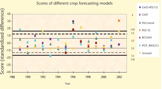
It is important to note at the very beginning of the present chapter that operational forecasting is done for different spatial scales (Gorski and Gorska,
1 Plant and animal pathologists do traditionally deal with
these issues, but they are not necessarily aware of the modern techniques (such as geostatistics) that are now familiar to most agrometeorologists.
2 The method applies mostly to high-value and predominately
wind-pollinated crops, such as grapes. Airborne pollen is sampled and calibrated against production in the surround-ing area. The method is currently underdeveloped regardsurround-ing the physico-physiological emission and capture of pollen by plants as a function of environmental conditions, transpor-tation of pollens by air, trapping efficiency, including trap behaviour, and the effect of atmospheric agents, especially rain.
2003). At the lowest end, the “microscale”, we have the field or the farm. Data are usually available with good accuracy at that scale. For instance, the breed or the variety is known, and so are the yield and the environmental conditions: soil type, soil depth, rate of application of inputs. The microscale is the scale of on-farm decision-making by individuals, irrigation plant managers, and so on.
The macroscale is the scale of the region, which is why forecasting for a district or province is usually referred to as “regional” forecasting. Regional fore-casts are at the scale of agricultural statistics. Regional forecasts are relevant for a completely different category of users, including national food security managers, market planners and traders, and so forth. At the macroscale, many variables are not known and others are meaningless, such as soil water-holding capacity.
Needless to say, the real world covers the spec-trum from macro- to microscales, but the two extremes are very well defined in terms of custom-ers and methods3. Several applications are at an
intermediate scale. They would include, for instance, certain types of crop insurance, the “livelihood analysis” that is now applied in many food security monitoring systems, fire monitor-ing systems, and so on.
Next, the links between forecasting and monitor-ing should be mentioned. Traditionally, monitoring is implemented by direct observation of the stage and condition of the organisms being monitored (type 1), or by observation of the envi-ronmental conditions that are conducive (or not) to the development of organisms (type 2)4. The
second type applies mostly to pests and diseases. Surprisingly, type 1 monitoring is often more expensive than type 2 because of elevated labour costs. On the other hand, when data are collected to assess environmental conditions, this is rela-tively close to forecasting as data requirements naturally overlap between type 2 monitoring and forecasting.
3 Time scales usually parallel spatial scales, with a decrease in
sampling frequencies when they refer to large areas.
4 A reviewer rightly underlines the similarities between
6.1.2 Forecasting techniques in general5
There are a variety of generic forecasting methods, most of which can somehow be applied to agrome-teorological forecasting as well (Petr, 1991). According to Armstrong (2001), “judgement pervades all aspects of forecasting”. This is close to a definition that one of the authors has frequently applied to crop yield forecasting, which can be seen as “the art of identifying the factors that determine the spatial and interannual variability of crop yields” (FAO, 2003a). In fact, given the same set of input data, different experts frequently come up with rather different forecasts, some of which, however, are demonstrably better than others, hence the use of the word “art”.
There appears to be no standard classification of forecasting methods (Makridadis et al., 1998; Armstrong, 2001). Roughly speaking, forecasting methods can be divided into various categories according to the relative proportion of judgement, statistics, models and data used in the process. Armstrong identifies 11 types of methods, which can be grouped as:
(a) Judgemental, based on stakeholders’ inten-tions or on the forecasters’ or other experts’ opinions or intentions. Some applications of this approach exist in agrometeorological fore-casting, especially when other factors, such as economic variables, play a part (for instance, the “Delphi expert forecasting method” for coffee described by Moricochi et al., 1995); (b) Statistical, including univariate (or extrapolation),
multivariate (statistical “models”) and theory-based methods. This is the category in which most agrometeorological forecasting belongs; (c) Intermediate types, which include expert
systems (basically a variant of extrapolation with some admixture of expert opinion) and analogies, which Armstrong places between expert opinions and extrapolation models. This is also covered in the present chapter. In this chapter, “parametric models” are considered to be those that attempt to interpret and quantify the causality links that exist between crop yields and environmental factors – mainly weather, farm management and technology. They include essentially crop simulation models6 and statistical7
5 Definitions used in the present chapter may differ from
those adopted in other scientific areas.
6 Also known as process-oriented models or mechanistic models.
7 For an overview of regression methods, including their
validation, refer to Palm and Dagnelie (1993) and to Palm (1997).
“models”, which empirically relate crop yield with assumed influential factors. Obviously, crop yield weather simulation belongs to Armstrong’s Theory-based Models.8 Non-parametric forecasting methods
are those that rely more on the qualitative description of environmental conditions and do not involve any simulation as such (Armstrong’s Expert Systems and Analogies).
6.1.3 Areas of application of
agrometeorological forecasts
6.1.3.1 Establishment of national and regional forecasting systems
There are a number of examples of institutionalized forecasting systems. As far as the authors are aware, they are never referred to as “agrometeorological forecasting systems”, even if many are built around some form of agrometeorological core (Glantz, 2004). Most forecasting and warning systems involv-ing agriculture, forests, fisheries, livestock, fires, commodity prices, food safety and food security, the health of plants, animals and humans, and so forth, do have an agrometeorological component.
Some forecasting systems are operated commer-cially, for instance, for high-value cash crops (coffee, sugar cane, oil palm), directly by national or regional associations of producers. The majority of warning systems, however, have been established by govern-ments or government agencies or international organizations, because of the high costs involved, the highly specific information needed for govern-ment programmes, or a lack of commercial interest (for example, in food security).
On the other hand, it is striking how few integrated warning and forecasting systems do exist. Clearly, fire forecasting, crop yield forecasting, pest forecasting and many other systems have various types of data and methods in common. Yet, they are mostly operated as parallel systems. For a general overview of the technical and institutional issues related to warning systems, refer to the above-mentioned volume by Glantz. Good examples of pest and disease warning systems can be found in Canada, where pest warn-ing services are primarily the responsibility of the provincial governments. In Quebec, warning serv-ices are administered under the Réseau d’avertissements phytosanitaires (RAP). The RAP was established in 1975; it includes 10 groups of experts and 125 weather stations and covers 12 types of crops. Warnings and other outputs from
the RAP can be obtained by e-mail, fax or the Internet (Favrin, 2000).
Warning and forecasting systems have recently undergone profound changes linked with the wide-spread access to the Internet. The modern systems permit both the dissemination of forecasts and the collection of data from the very target of the fore-casts. Agricultural extension services usually play a crucial role in the collection of data and the dissem-ination of analyses of forecasting systems (FAO, 2001b, 2003a). In addition to providing inputs, users can often interrogate the warning system. Light leaf spot (Pyrenopeziza brassicae) is a serious disease of winter oilseed rape crops in the United Kingdom. At the start of the season, a prediction is made for each region using the average weather conditions expected for that region. Forecasts avail-able to growers over the Internet are updated periodically to take account of deviations in actual weather from the expected values. The recent addi-tion of active server page technology has allowed the forecast to become interactive. Growers can input three pieces of information (cultivar choice, sowing date and autumn fungicide application information), which are taken into account by the model to produce a risk assessment that is more crop- and location-specific (Evans et al., 2000). Before they become operational, forecasting systems are often preceded by a pilot project to fine-tune outputs and consolidate the data collection systems. A good example is provided by the Pilot Agrometeorological Forecast and Advisory System (PAFAS) in the Philippines because of the number of institutional users involved. The general objec-tives of the proposed PAFAS were to provide meteorological information for the benefit of agri-cultural operations (observation and processing data) and to issue forecasts, warnings and advisories of weather conditions affecting agricultural produc-tion within the pilot area (Lomotan, 1988).
This section emphasizes that few warning systems can properly assess the damage caused by extreme agrometeorological events to the agricultural sector. Such damage may be significant; it may reach the order of magnitude of the gross national product (GNP) growth. For many disaster-prone countries, agricultural losses due to exceptional weather events are a real constraint on their overall economy. When infrastructure or slow-growing crops (such as plantations) are lost, the indirect effects of disasters on agriculture may last long after the extreme event takes place. The time needed to recover from some extreme agrometeor-ological events ranges from months to decades.
6.1.3.2 Farm-level applications 6.1.3.2.1 Overview
Farmers in all cultures incorporate weather and climate factors into their management processes to a significant extent. Planting and crop selection are functions of the climate and of the normal change of the seasons. Timing of cultural operations, such as cultivation, application of pesticides and fertilizers, irrigation and harvesting, is strongly affected by the weather of the past few days and in anticipation of the weather for the next few days. In countries with monsoonal climates, planting dates of crops depend on the arrival of the monsoonal rains. Operations such as haymaking and pesticide application will be suspended if rain is imminent. Cultivation and other cultural practices will be delayed if the soils are too wet. The likelihood of a frost will trigger frost-protection measures. Knowledge of imminent heavy rains or freezing rains will enable farmers to shelter livestock and to protect other farm resources. Irrigation scheduling is based on available soil moisture9 and crop water-use rate, both of which are
functions of the weather. Farmers have always been very astute weather watchers and are quick to recognize weather that is either favourable or unfavourable to their production systems.
This traditional use of weather in farm manage-ment is significant, but it is not the only use of weather information in farm management. In addi-tion to these well-known direct effects of weather on agricultural production, weather-wise farm management takes into account the indirect effects of weather. Temperature determines the rate of growth and development10 of insects, temperature
and humidity combinations influence the rate of fungal infection, evapotranspiration rates deter-mine water-use rates and irrigation schedules, and radiation and moisture availability are important in the rate of nutrient uptake by crops. These effects of weather on production are not directly observable and are not the basis of a “yes” or “no” or “don’t” type of decision, but they have significant economic potential when incorporated into the farm manage-ment process (McFarland and Strand, 1994).
9 The terms “soil moisture” and “soil water content” are used
interchangeably.
10 Growth refers to the accumulation of biomass or weight by
organisms. It is a quantitative phenomenon. Development, on the other hand, refers to the qualitative modifications that take place when organisms grow: formation of leaves, differentiation of flowers, successive larval stages of some insects, and so forth. While this chapter deals mainly with growth forecasting, there are applications in which develop-ment receives the most attention (see 6.5.5).
Consequently, regarding the importance of weather forecasting in farm management, the following aspects are crucial:
(a) Current weather information (for example, forecasts) must be provided routinely to the decision-maker by an outside agency. Farmers cannot observe or develop all the necessary information;
(b) Managers have to incorporate less-than-perfect weather information into their deci-sion processes;
(c) Farmers can develop and evaluate their deci-sion processes for direct effects of weather, but must rely on outside expertise for decision support regarding indirect effects of weather. The use of weather information in farm manage-ment in developing nations is particularly valuable when the level of production inputs is increased. Virtually all the inputs that characterize increased production are weather sensitive and most are also weather information sensitive. Irrigation, fertiliza-tion, pesticides, fungicides and mechanization are all more weather sensitive than traditional agricul-tural operations. In these cases, the incorporation of weather into the management process should be included when the technology involving the appro-priate inputs is transferred. For example, when the use of insecticides for crop protection is imple-mented, the full use of weather information in pest management and the effects of weather on the application should be included in the technology transfer process.
Weather contingency planning for the farm level is not well developed. Swaminathan (1987) recom-mended that a “Good Weather Code” be developed, in addition to contingency plans based on drought or monsoon failure. Areas that are chronically drought-prone need measures to promote moisture retention and soil conservation.
Pest management is both weather sensitive and weather information sensitive. Weather sensitivity is primarily defined as the effects of wind, temperature and precipitation on application of the pesticide. The weather-sensitive aspects of pest management are supported by the more or less conventional weather information from the mass media. If the farmer is aware of the nature of the weather sensitivity, the existing decision processes should be sufficient. Scheduling of the times of application to avoid unfavourable winds or anticipated rains is within the farmer’s traditional use of weather information. Weather information sensitivity is primarily the optimal timing of the pesticide as a function of temperature effects on
insect population dynamics and the crop growth rates. Insects are poikilothermic organisms, whose rate of growth and development is determined by the heat energy of the immediate environment. Temperature, as a measure of available heat energy, is used extensively to derive insect growth rates and development simulation models.
6.1.3.2.2 Response farming applications
“Response farming” is a methodology developed by Stewart (1988) and based on the idea that farm-ers can improve their return by closely monitoring on-farm weather and by using this information in their day-to-day management decisions. The emphasis here is on the use of quantitative current data, which are then compared with historical information and other local reference data (infor-mation on soils, and so on). This is a simple variant of the what-if approach. What about planting now if only 25 mm of rainfall has been recorded from the beginning of the season? What about using 50 kg N-fertilizer if rainfall so far has been scarce and the fertilizer will increase the crop water requirement and the risk of a water stress?
The method implies that, using the long-term weather series, decision tools (usually in tabular or flow-chart form) have been prepared in advance. They are based on the following information:
(a) Knowledge of local environmental/agricul-tural conditions (reference data);11
(b) Measurement of local “decision parameters” by local extension officer or farmer;
(c) Economic considerations.
In the latter, the decision tools must be prepared by national agrometeorological services in collaboration with agricultural extension services and subsequently disseminated to farmers. This operation will be the most difficult in practice (WMO/CTA, 1992).
A similar concept to response farming is flex cropping; it is used in the context of a crop rotation where summer fallow is a common practice, especially in dry areas, such as the Canadian prairies. Rotations are often described as 50:50 (1 year crop, 1 year fallow) or 2 in 3 (2 years crop, 1 year fallow). The term flex crop has emerged to describe a less rigid system in which a decision to re-crop (or not) is made each year based on available soil water content and the prospect of
11 A simple example of this could be a threshold of air moisture
or sunshine duration to decide on pest risk, or a threshold of salt content of water to decide on irrigation-salinity risk. Normally, other parameters (economic) also play an impor-tant part.
getting good moisture during the upcoming growing season (Zentner et al., 1993; P. Dzikowski and A. Bootsma, personal communication).
Weisensel et al. (1991) have modelled the rela-tive profitability and riskiness of different crop decision models that might be used in an exten-sive setting. Of particular interest is the value of information added by the availability of spring soil moisture data and by dynamic optimization. The simulation has shown that flex cropping based on available soil moisture at seeding time is the most profitable cropping strategy. The authors stress the importance of accurate soil water content information.
6.1.3.2.3 Farm management and planning (modern farming)
Farmers have been using weather forecasts directly for a number of years to plan their operations, from planting wheat to harvesting hay and spraying fungicides. Simulation models, however, have not really entered the farm in spite of their potential. The main causes seem to be a mixture of lack of confidence and lack of data12 (Rijks, 1997).
Basically three categories of direct applications of forecasts can be identified:
(a) What-if experiments to optimize the economic return from farms, including real-time irriga-tion management. This is the only area in which models are well established, including models in some developing countries (FAO, 1992);
(b) Optimization of resources (pesticides, ferti-lizer) in the light of increasing environmental concern (and pressure);
(c) Risk assessment, including the assessment of probabilities of pest and disease outbreaks and the need to take corrective action.
Contrary to most other applications, on-farm real-time operations demand well-designed software that can be used by the non-expert, as well as a regular supply of data. In theory, some inputs could be taken automatically from recording weather stations, but specific examples are rare. A publication by Hess (1996) underlines the sensitivity of an irrigation simulation program to errors in the on-farm weather readings.
12 For developing countries, one of the reviewers of this
docu-ment adds the very basic “lack of electricity”, lack of comput-ers, lack of knowledge about the existence of models, not to mention the fact that models are rarely developed for the farming community.
Systems have been described in which some of the non-weather inputs come from direct measure-ment. Thomson and Ross (1996) describe a situation in which model parameters were adjusted on the basis of responses by soil water sensors to drying. An expert system determined which sensor read-ings were valid before they could be used to adjust parameters.
Irrigation systems have a lot to gain from using weather forecasts rather than climatological aver-ages for future water demand. Fouss and Willis (1994) show how daily weather forecasts, including real-time data on the likelihood of rainfall from the daily National Weather Service forecasts, can assist in optimizing the operational control of soil water and scheduling agrochemical applications. The authors indicate that the computer models will be incorporated into decision support models (Expert Systems) that can be used by farmers and farm managers to operate water–fertilizer–pest manage-ment systems.
Cabelguenne et al. (1997) use forecast weather to schedule irrigation in combination with a variant of the Environmental Policy Integrated Climate model (EPIC, formerly the Erosion Productivity Impact Calculator). The approach is apparently so efficient that discrepancies between actual conditions and weather forecasts led to a difference in tactical irriga-tion management.
This section ends with an interesting example of risk assessment provided by Bouman (1994), who has determined the probability distribution of rice yields in the Philippines based on the probability distribu-tions of the input weather data. The uncertainty in the simulated yield was large: there was a 90 per cent probability that simulated yield was between 0.6 and 1.65 times the simulated standard yield in average years.
6.1.3.3 Warning systems, especially for food security13
Many warning systems target both individual and institutional users, although governments are usually the main target of warnings for food security. In
13 Largely taken from WMO, 1997. Although pests and diseases
are not the focus of this section, it is worth noting that many models developed in the general field of plant pathology can often be associated with the crop-weather models in impact assessments and warning systems. For an overview of such models, refer to Seghi et al. (1996). Most of them are typical developed-country applications, because both data availabil-ity and good communications permit their implementation in a commercial farming context.
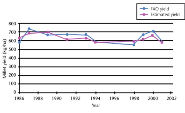
many developing countries, farmers still practice subsistence farming, that is, they grow their own food, and depend directly on their own food produc-tion for their livelihood. Surpluses are usually small; they are mostly commercialized in urban areas (the urban population constitutes about 30 per cent of the total population in Africa). Yields tend to be low: in Sahelian countries, for instance, the yields of the main staples (millet and sorghum) are usually in the range of 600 to 700 kg/ha during good years. Interannual fluctuations are such that the national food supply can be halved in bad years or even drop to zero in some areas.
This is the general context in which food surveil-lance and monitoring systems were first established in 1978. Currently, about one hundred countries on all continents operate food security warning systems; the names of these systems vary, but they are generally known as (Food) Early Warning Systems (EWSs). They contribute to:
(a) Providing national decision-makers with advance notice of the magnitude of any impending food production deficit or surplus; (b) Improving the planning of food trade,
market-ing and distribution;
(c) Establishing coordination mechanisms among relevant government agencies;
(d) Reducing the risks and suffering associated with the poverty spiral.
EWSs cover all aspects from food production to marketing, storage, national imports and exports, and consumption at the household level. Monitoring weather and estimating production have been essential components of the system from the outset, with the direct and active involvement of National Meteorological Services. Over the years, the methodology has kept evolving, but crop moni-toring and forecasting remain central activities:
(a) Operational forecasts are now mostly based on readily available agrometeorological or satellite data, and sometimes a combina-tion of both. They do not depend on expen-sive and labour-intenexpen-sive ground surveys and are easily revisable as new data become available;
(b) Forecasts can be issued early and at regu-lar intervals from the time of planting until harvest. As such, they constitute a more meaningful monitoring tool than the moni-toring of environmental variables (rainfall monitoring, for instance);
(c) Forecasts can often achieve a high spatial resolution, thus leading to an accurate estimation of areas and number of people affected.
Due to the large number of institutional and tech-nical partners involved in EWSs, interfacing among disciplines has been a crucial issue. For instance, crop prices are usually provided as farm-gate or marketplace prices, food production and popula-tion statistics cover administrative units, weather data correspond to points (stations) not always representative for the agricultural areas, satellite information comes in pixels of varying sizes, and so forth. Geographical Information System (GIS) tech-niques, including gridding, have contributed to improving links in the “jungle” of methods and data (Gommes, 1996).
6.1.3.4 Market planning and policy
Advance knowledge of the likely volume of future harvests is a crucial factor in the market. Prices fluc-tuate as a function of the expected production14
(read: forecast production), with a large psychologi-cal component.
In fact, prices depend more on the production that the traders anticipate than on actual production. Accurate forecasts are, therefore, a useful planning tool. They can also often act as a mechanism to reduce speculation and the associated price fluctua-tions, an essential factor in the availability of food to many poor people.
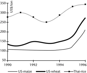
Figure 6.1 shows that wheat prices increased from about US$ 150 per tonne in 1993 to about US$ 275 per tonne at the end of 1995. The main causes were the policy of both the United States and the European Union to reduce stocks (stocks are expensive to maintain), and the poor prospect for the 1995/1996 winter wheat in the United States and European Union. Maize, a summer crop, was affected by “contagion”. Had the forecasts been more accurate and reliable, it is clear that the prices would have remained more stable: they peaked around May 1996, and then returned to normal values.
A similar, but more dramatic situation occurred with coffee prices in 1977 when they reached an all-time high due to low stocks and frost in some of the main producing areas in Brazil (Brazil produces about 28 per cent of the world output, of which more than half comes from the states of São Paulo and Minas Gerais).
Commercial forecasts are now available by subscrip-tion. CROPCAST, for instance, provides estimates not only for yields, but also for production, areas, stocks,
14 The main factors affecting prices are world production
crop condition and futures prices (http://www.mdafed-eral.com/mda-earthsat-weather/crop cast-ag-services). On a local scale, many food-processing plants depend on production in their area, which is linked to the seasonality of production for most crops (canning of fruit and vegetables, sugar from sugar beet, cotton-fibre processing, oil from sunflowers and oil palm15,
and so forth). It is important to have accurate fore-casts for the volume to be processed and for the timing of operations.
6.1.3.5 Crop insurance
Crop insurance is one of the main non-structural mechanisms used to reduce risk in farming; a farmer who insures his crop is guaranteed a certain level of crop yield or income, which is equivalent, for instance, to 60 or 70 per cent of the long-term average. If, for reasons beyond the farmer’s control, and in spite of adequate management decisions, the yield drops below the guarantee, the farmer is paid by the insurer a sum equivalent to his loss, at a price agreed before planting.
Crop insurance schemes can be implemented relatively easily when there is sufficient spatial
15 Oil palm and other palms pose a series of very specific
fore-casting problems due to the long lag between flower initia-tion and harvest. This period usually covers three years or more. In addition, probably more than in other plants, qual-itative factors are critical, for instance the effect of tempera-ture on sex differentiation (only female flowers produce seeds, thus oil). See Blaak (1997) for details.
variability of an environmental stress (such as with hail), but they remain extremely difficult to implement for some of the major damaging factors, such as drought, which typically affect large areas, and sometimes entire countries. One of the basic tools for insurance companies is risk analysis (Abbaspour, 1994; Decker, 1997). Crop forecasting models play a central part: when run with historical data, they provide insight into the variability patterns of yield. Monte Carlo methods play an important part in this context, either in isolation or in combination with process-oriented or statistical models. Almost all major models have been used in a risk assessment context, including the World Food Study, or WOFOST, model (Shisanya and Thuneman, 1993) and the Australian Sugar Cane, or AUSCANE, model (Russel and Wegener, 1990), among others (de Jager and Singels, 1990; Cox, 1990).
Many of the papers presented in July 1990 at the international symposium in Brisbane, Australia, on Climatic Risk in Crop Production: Models and Management in the Semi-arid Tropics and Subtropics, are relevant in the present context. The use of crop insurance is not widespread in many developing countries and transition economies, although the World Bank and the World Food Programme are currently setting up schemes that should considerably facilitate food security-related operations by resorting to insurance-based emergency funds. The difficulty in implementing insurance schemes to assist smallholders is best explained by the fact that many farmers live at the subsistence level, that is, they do not really enter commercial circuits. Rustagi (1988) describes the general problem rather well. For instance, insurance companies insure a crop only if the farmer conforms to certain risk-reducing practices, such as early planting. The identification of the “best” planting dates constitutes a direct application for process-oriented crop-weather models. The paper quoted by Shisanya and Thuneman (1993) uses WOFOST to determine the effect of planting date on yields in Kenya.
An interesting example regarding both forecasting of the quality of products and insurance is given by Selirio and Brown (1997). The authors describe the methods used in Canada for the forecasting of the quality of hay: the two steps include the forecasting of grass biomass proper, and subsequent forecasting of the quality based essentially on the drying conditions. One of the reasons models have to be used is the absence of a structure that measures, stores and markets
US$/ton 350 300 250 200 150 100 50 1990 1992 1994 1996 US-maize US-wheat Thai-rice
Figure 6.1. Variations in wheat, rice and maize prices between 1990 and 1996 (fixed 1996 CIF1 US$ prices). The ticks on the X-axis represent the
forage crops that is comparable to what is available for grain crops. In addition, field surveys are significantly more expensive to carry out than forecasts.
Crop forecasts used in crop insurance schemes must conform to several criteria that are less relevant for other applications:
(a) Tamper-resistance: Potential beneficiaries of the insurance should not be in a position to directly or indirectly manipulate the yield estimate; (b) Objectivity: Once the methodology has been
defined in precise terms, the forecasts can be calculated in an objective manner;
(c) Special calibration techniques: A “poor year” is defined as a year in which condi-tions are bad enough to trigger the payment of claims to insurance subscribers. A “poor year” can be defined based on at least three approaches: (1) absolute yield levels (possibly the most appropriate choice for food security); (2) a percentage of the average local yield (a “fair” choice as expectations are different in high-potential and low-potential areas; and (3) probability of exceeding a specific yield (this usually gives “good” results in terms of statistical significance). Rather than the statis-tical strength of the correlation between yield and crop-weather index, it is the number of false positives (good year assessed to be poor) and false negatives (poor year assessed as good) that constitutes the most important criterion; (d) Insensitivity to missing data: The best way to
circumvent the occurrence of missing spatial data is to use gridded information that is not too sensitive to individual missing stations, provided sufficient data points are avail-able and the interpolation process takes into account topography and climatic gradients; (e) Publicity: Methodology has to be made available
and understandable to potential subscribers of the insurance to build up mutual trust. Yield forecasts must be published regularly, for instance in national agrometeorological bulletins and through other channels, such as Websites.
6.2 VARIABLES USED IN AGROMETEOROLOGICAL FORECASTING
6.2.1 Overview
In agrometeorological forecasting, a statistic (for exam-ple, yield) that is being forecast depends very often on a number of variables belonging to different technical
areas, from the socio-economic and policy realms to soil and weather. The idea behind agrometeorological forecasting is first to understand which factors play a part in the interannual variability of the forecast parameter, and then to use the projections for those factors to estimate future yield.
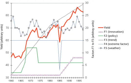
A hypothetical example is shown in Figure 6.2: innovation and trend are mainly associated with technology, such as breeds and improved harvest-ing techniques. Policy covers essentially economic decisions (such as prices) that lead producers to increase or decrease inputs or, in general, to modify management practices in response to the socio-economic environment. Extreme factors and weather are separated here for two reasons: (1) not all extreme factors are weather related and (2) for those that are, the mechanism of their interaction with agricultural production is rather different from the mechanisms usually at play under “normal” conditions (see 6.4.5).
“Weather” is supposed to remain within the normal physiological range of variations: organisms can respond in a predictable way, following well-established and generally well-understood patterns (such as photosynthesis response to light intensity, transpiration of animals as a function of atmospheric moisture content and temperature). On the other hand, “extreme” factors exceed the normal range of physiological response.
Sections 6.2.2. to 6.2.5 below provide a list of variables that are frequently used for agrometeorological forecasting. For many years, agrometeorological forecasting has resorted to raw weather variables as the main predictors. The current tendency is to focus on value-added variables, that is, variables that have undergone some agrometeorological pre-processing using various models. Two such variables are soil moisture and actual evapotranspiration (ETA). Both are estimated using models. Soil moisture, for instance, constitutes a marked improvement over rainfall, because it assesses the amount of water that is actually available for crop growth and takes into account rainfall amount and distribution. Without entering into a discussion of indices and indicators, one can regard soil moisture as a complex derived indicator, a value-added forecasting variable. There is no standard method to select variables used for crop forecasting, as clearly shown by the number and variety of approaches that have been developed for agrometeorological forecasting since the 1950s. The inclusion of limiting factors in the equations is characteristic of the existing methods.
These factors vary in relation to crop, cultivation technique, soil and climate conditions. For exam-ple, equations for arid regions include moisture provision indices (productive water reserves in the soil, precipitation, and so forth), whereas for rice (cultivated by flooding), atmospheric temperature and solar radiation values serve as the parameters. Data on crop conditions (number of stalks, leaf surface area, plant heights) are used in an array of methods. The majority of existing theoretical and applied yield forecast methods are based on statis-tical analysis of agro meteorological observation data and on correlation and regression analyses. The equations derived in these instances should refer only to specific regions and cannot be used in others.
Many mathematical models, however, in attempt-ing to represent the complex processes of yield formation by allowing for many factors (including physiological processes, the stereometry of a crop, energetics of photosynthesis, and microflora activ-ity in the soil), cannot be used at the present time to forecast yields in production conditions involv-ing millions of hectares (regional forecasts). The primary reason for this is that it is not feasible to organize observations of these complex processes. Another factor is the efficiency required for synthe-sizing a forecast. Some forecast models are not efficient in the use of the simplest and least labori-ous forms of calculation, which permit the rapid retrieval of vast amounts of information even with a limited number of predictors.
Further refinement of the existing yield forecast methods requires considerable improvements of the reference data, namely, the agricultural statis-tics used for calibration, including improved maps of regional yield patterns. The extent of damage caused by pests and diseases, which is itself related to weather conditions, should be included as a correction factor.
Any deficiencies in the accuracy of agrometeoro-logical forecasting depend on (a) how well the initial observations represent regional condi-tions; (b) how homogeneous the regional conditions (climate, soil characteristics, and so on) are; (c) how accurate the observations them-selves are; and (d) how sensitive the model is to the variations in the agrometeorological variable being forecast (see 6.3.2).
Long- or medium-range weather forecasting methods have not yet reached the level of accuracy desirable for operational use, particularly in tropical countries. The temporal instability of some predictors does not allow the continued use of such models over a long time without change. The periodic revision of models also has to be viewed in the light of the possible impact of global warming and climate change on the interannual variability of meteorological parameters. In the case of medium-range weather forecasts, their accuracy level has improved potentially in extra-tropical countries (see 6.2.5.3).
Figure 6.2. A hypothetical example showing how yield depends on various factors
Yield (arbitrar y units) Yield F1 (innovation) F2 (policy) F3 (trend) F4 (extreme factor) F5 (weather)
6.2.2 Technology and other trends
Most agricultural systems are affected by technology trends and, sometimes, variations that are short-lived and not necessarily related to environmental conditions.16 One should stress
that some biological production systems display regular variations that are endogenous or due to management practices. Some crops, for instance coffee in Kenya, display an alternating pattern of high and low yields (Ipe et al., 1989.) Another essential point is that trends may be difficult to detect in the presence of very high weather variability. Before the effect of weather conditions can be assessed, it is necessary to remove the trend (that is, to “detrend” the time series) and other non-weather factors.
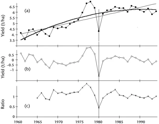
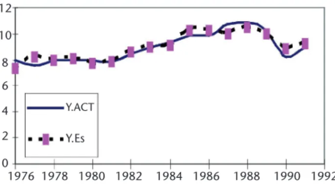
The example in Figure 6.3 (Republic of Korea) shows a typical upward trend due to improved technology (varieties, management, inputs), as well as the linear and quadratic trend. The coefficients of determination
16 A fundamental assumption in model-building is that the
behaviour of the agricultural production system is stationary or invariant over time. If this is not so, regression methods are generally invalid.
Figure 6.3. Yield of total paddy in the Republic of Korea between 1960 and 1994 (based on FAO statistics). The top curve (a) indicates the actual yields with their linear and quadratic trends;
the middle curve (b) is the detrended yield, that is, the difference (residual) between actual yield and the quadratic trend; the lower curve (c) shows the ratio between the
yield of year N and the average of the 4 years from N-1 to N-4.
Ratio Yield (t/ha) Yield (t/ha) (a) (b) (c) 1960 1965 1970 1975 1980 1985 1990 6.5 6 5.5 5 4.5 4. 3.5 0.5 0 –0.5 –1 1 0.5 0
amount to 0.71 and 0.74, respectively. The coefficient achieved with the “best” trend model (a sigmoid, not shown) amounts to 0.80. Within the remaining 20 per cent, weather probably accounts for about half. The sharp drop in 1980 was due to severe low temperatures around the heading through early ripening stage. Tong-il varieties are high-yielding hybrids that are very sensitive to abnormally cool temperatures due to the failure in pollination. In the late 1970s, the weather had been mostly favourable to rice cultivation, especially to the Tong-il type (B. L. Lee, personal communication). Threshold effects (such as the temperature effect mentioned above) are extremely difficult to fore-cast by most techniques. Non-parametric methods have an advantage over other approaches in this respect.
The middle curve shows the detrended yield (using the quadratic trend). This is the yield that will be used to calibrate a regional crop forecasting model. The lower curve shows the ratio between the yield of the current year and the average of the yields of the four preceding years, assuming that the trend is not significant over such a short period. The advan-tage of this approach is that no trend has to be
determined, and no hypothesis has to be made about the shape of the trend. Some studies deal with the technology trend by predicting the differ-ence between this year’s yield and last year’s yield (first order difference). As the method seems to ignore background climate, it is not further discussed here.
A number of methods can be used to cope with trends. The “best” approach is, of course, to include in the forecasting model some variables that contribute to the trend, whenever independent information is available about the technology component (such as the number of tractors per hectare or actual fertilizer use per hectare). One of the main factors behind trends, however, is the gradual change in the mix of varieties, which remains difficult to handle. In addition to the trend removal techniques illustrated above (largely drawn from Gommes, 1998a, 1998b), it is also possible to include time as a variable in statistical forecasts. The number of existing empirical methods devel-oped to handle this problem is another illustration of the fact that crop forecasting relies frequently on the experience of the forecaster (it is “art”, as mentioned several times).
6.2.3 Soil water balance: moisture
assessment and forecast
6.2.3.1 Presentation
Soil moisture content at sowing and fruiting times is closely related to the emergence, growth and productivity of plants. In order to use irrigation efficiently, it is necessary to know the actual amount of water required to make up the depleted portion of the soil moisture at the various crop growth stages. Techniques have been developed accordingly for the forecasting – or assessment – of available moisture in a 1 m layer of soil at the beginning of the growing period. This is of great assistance to farm operators and agricultural planning agencies as a forecasting variable. This forecast is often based on climatological water balance methods or empirical regression-type equations.
An assessment of moisture conditions is based on past and present climatological data (such as precip-itation, radiation, temperature, wind) with or without the use of soil moisture measurements. An extrapolation of this current estimate into the near future is possible through the use of long-term averages or other statistical values of the above meteorological data in the water balance equation. In addition, a soil water content forecast equation
is based on a statistical analysis of recorded soil water content data related to one or several other agrometeorological variables. This approach uses, sometimes on a probability basis, the occurrence of events in the past for extrapolation into the near future. Water balance methods use the following basic equation:
P – Q – U – E – ∆W = 0 (6.1)
where P is the precipitation or irrigation water supply, Q is runoff, U is deep drainage passing beyond the root soil, E is evapotranspiration and ∆W is change in soil water storage.
Each of the terms in this equation has special problems associated with its measurement or estimation. In most practical applications it is assumed that certain terms, such as Q or U, are negligible. Another assumption is that ∆W, at least over large areas and extended periods, can be set equal to zero. For short-term or seasonal applications, an approximate value of ∆W, that is, the soil water storage at the beginning and end of the period under consideration, is required. Such a value can be obtained from soil moisture measurements (WMO, 1968) but, more practically, from using climatic data in appropriate estimation techniques, such as those by Thornthwaite, Penman, Fitzpatrick, Palmer, Baier-Robertson or Budyko (WMO, 1975). 6.2.3.2 Soil water balance for dryland crops
An example of the application of the water balance approach to estimating soil moisture, as well as the stress period for dryland crops, is the cumulative water balance developed by Frère and Popov (1979), based on 10-day values of the precipitation and potential evapotranspiration. The water balance is the difference between precipitation received by the crop and the water lost by the crop and the soil through transpiration and evaporation, which is a fraction of the potential evapotranspiration. The water retrieval in the soil is also taken into account. The basic formula is as follows:
Si = Si –1 + Pi – WRi (6.2)
where Si is the water retained in the soil at the end of
the 10-day period; Si–1 is the water retained in the soil
at the onset of the 10-day period; Pi is precipitation
during the 10-day period; WRi represents the water
requirement of the crop during the 10-day period. WRi in turn is defined as
in which PETi is the potential evapotranspiration
during the 10-day period and Kcri is the crop
coeffi-cient during the 10-day period.
Regression-type techniques for estimating soil mois-ture or changes in the water reserves have been developed in many countries for specific crops, soils, climates and management practices. The equations used take the following form:
ΔΔZ = aW + bT + cP + d (6.4)
where ΔΔZ is the change in soil moisture of a 1 m layer of soil over a 10-day period; W represents soil moisture reserves at the beginning of the 10-day period; T denotes mean air temperature over the 10-day period and P is the total precipitation over the 10-day period; a, b, c and d are regression coefficients.
Das and Kalra (1992) developed a multiple regres-sion equation to estimate soil water content at greater depths from the surface layer data:
S = 0.22502 (d – d0) +
S0 (1 – 0.000052176 (d – d0)2) – 2.35186 (6.5)
where S is the soil moisture at depth d and S0 is the soil moisture at or near the surface layer whose depth is d0. This equation was fitted to the mois-ture data under wheat grown in India under various irrigation treatments.
6.2.4 Actual evapotranspiration (ETA)
In the mid-1950s de Wit was among the first to recognize that there is a direct link between transpiration and plant productivity (van Keulen and van Laar, 1986). Transpiration can be limited due to a short supply of water in the root zone, or by the amount of energy required to vaporize the water. It can be said that plant growth (biomass accumulation) is driven by the available energy, but that plants “pay” for the energy by evaporating water. This is one of the basic “tenets” of agro- meteorology.
Relative evapotranspiration is defined by the equa-tion Q = LE/LEm and relative assimilation by Rass = F/Fm. LE and F are evapotranspiration and
assimi-lation, respectively. The subscript in LEm and Fm
denotes maximum values. A plot of relative assim-ilation Rass as a function of relative transpiration Q
is close to linear when Q values are relatively high (at least Q > 0.6). If other effects can be assumed to be constant, the relative assimilation over a day (measured as biomass accumulation) is directly
related to relative evapotranspiration (approxi-mated by ETA):
Daily biomass accumulation ≈ K * ETA (6.6) ETA is one of the best forecasting variables in absolute terms because, as indicated above, it is directly related to biomass production. But it is also useful owing to its synthetic nature (it includes radiation as one of its main driving forces). And finally, the linearity between ETA and biomass assimilation has been shown repeat-edly to hold across many scales, from leaf to plant, to field and to a region.
The persistence of the relationship between ETA and biomass accumulation across spatial scales derives essentially from the fact that both CO2
absorption and water transpiration take place through the same anatomic structure, the stomata. Maximum evapotranspiration (LEm) and maximum assimilation (Fm) occur when the stomata are completely open, and both are close to zero when the stomata are closed. LE is the evaporative heat loss (J m–2 d–1), the product of E, the rate of water
loss from a surface (kg m–2 d–1) and L, the latent
heat of vaporization of water (2.45 106 J kg–1 ).
It is recommended that actual ET be included as one of the variables in crop forecasting methods using multiple regression. Alternatively, variables derived from ETA are also often resorted to, for instance, the ratio between actual ET and potential ET (Allen et al., 1998). The Cuban early warning system for agricultural drought has been using this index because of its direct relation with crop yields (Rivero et al., 1996; Lapinel et al., 2006). There are other related indices, such as Riábchikov’s index (Riábchikov, 1976), that can be used in climate change impact assessments. As ETA cannot be meas-ured directly in most cases, it is best estimated using a water balance, as explained in 6.2.3.2.
6.2.5 Various indices as measures of
environmental variability
6.2.5.1 Various drought indices
6.2.5.1.1 Overview
Drought indices can be quantified using a variety of relationships involving annual17 climatic values
and long-term normals. The majority of the indices reflect the meteorological drought but not necessar-ily the shortage of water for agriculture. The problem
of agricultural drought pertains to physical and biological aspects of plants and animals and their interactions with the environment. Since growth (biomass accumulation) is a complex soil–plant– environmental problem, agrometeorological drought indices18 must reflect these phenomena
truly and accurately.
The indices can, however, provide useful variables when assessing the extent to which plants have been adversely affected by the moisture deficiency, taking into consideration supply and demand of soil water content. The soil water deficiency during the growing season may result in a partial or complete loss of crop yield. But the rainfall amount below which a reduced crop is considered drought-stricken depends on the degree to which a crop can withstand the moisture deficiency, as well as the stage and state of the crop. The time step used to derive the drought indices is crucial. A day or month may not be suitable. A pentad or weekly values are usually appropriate. These indices can also serve specific purposes, such as irrigation scheduling and drought management.
6.2.5.1.2 Palmer drought severity index
The Palmer drought severity index (PDSI) (Palmer, 1968) relates the drought severity to the accumu-lated weighted differences between actual precipitation and the precipitation requirements of evapotranspiration. The PDSI is based on the concept of a hydraulic accumulating system and is actually used to evaluate prolonged periods of abnormally wet or dry weather.
The index is a sum of the current moisture anomaly and a portion of the previous index, so as to include the effect of the duration of the drought or wet spell. The moisture anomaly is the product of a climate-weighted factor and the moisture depar-ture. The weighted factor allows the index to have a reasonably comparable significance for different locations and time of year.
The moisture departure is the difference between water supply and demand. Supply is precipitation and stored soil moisture, and demand is the potential evapotran-spiration, the amount needed to recharge the soil, and runoff needed to keep the rivers, lakes and reservoirs at a normal level. The runoff and soil recharge and loss are computed by keeping a hydrological account of moisture storage in two soil layers. The surface layer
18 The Website of the National Drought Mitigation Center
(http://drought.unl.edu/) has many useful definitions and data relating to drought.
can store 2.54 cm, while the available capacity in the underlying layer depends on the soil characteristics of the division being measured. Potential evapotranspi-ration is derived from Thornthwaite’s method (Thornthwaite, 1948).
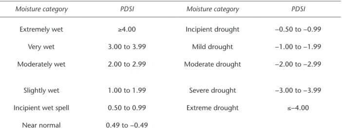
Note, however, that Thornthwaite’s method is not recommended for all climate conditions. Variants of the PDSI using Penman–Monteith potential evapotranspiration or modified water balances have also been used (Paulo and Pereira, 2006; Pereira et al., 2007; Szalai and Szinell, 2000). The index is measured from the start of a wet or dry spell and is sometimes ambiguous until a weather spell is estab-lished. Table 6.1 contains the Palmer drought index categories. A week of normal or better rainfall is welcome, but may be only a brief respite and not the end of a drought. Once the weather spell is established (by computing a 100 per cent “probabil-ity” that the opposite spell has ended), the final value is assigned. This is not entirely satisfactory, but it does allow the index to have a value when there is a doubt that it should be positive or negative.
One aspect that should be noted is that the demand part of the computations includes three input parameters – potential evapotranspiration, recharge of soil moisture, and runoff – any one of which may produce negative values. If only enough rain fell to satisfy the expected evapotranspiration, but not enough to supply the recharge and runoff, then a negative index would result. If such an odd situa-tion continued, agriculture would progress at a normal pace but a worsening drought would be indicated. Then if rainfall fell below the minimum needed for agriculture, crops would suffer drastic and rapid decline because there would be no reserve water in the soil.
6.2.5.1.3 The crop moisture index
Palmer (1968) developed the crop moisture index from moisture accounting procedures used in calcu-lations of the drought severity index to measure the degree to which moisture requirements of growing crops were met during the previous week. The crop moisture index gives the status of purely agricul-tural drought or moisture surplus affecting warm-season crops and field activities and can change rapidly from week to week.
The index is the sum of the evapotranspiration anomaly, which is negative or slightly positive, and the moisture excess (either zero or positive). Both terms take into account the value of the previous week. The evapotranspiration anomaly is weighted
to make it comparable for different locations and times of the year. If the potential moisture demand exceeds available moisture supplies, the index is negative. If the moisture meets or exceeds demand, the index is positive. It is necessary to use two sepa-rate interpretations because the resulting effects are different depending on whether the moisture supply is improving or deteriorating.
General conditions are indicated and local varia-tions caused by isolated rains are not considered. The stage of crop development and soil type should also be considered in using this index. In irrigated regions, only departures from ordinary irrigation requirements are reflected. The index may not be applicable for seed germination, for shallow-rooted crops that are unable to extract the deep or subsoil moisture from a 1.5 m profile, or for cool-season crops growing when average temperatures are below 12.5°C.
6.2.5.1.4 The standardized precipitation index (SPI)
The SPI was designed to be a relatively simple, year- round index applicable to all water supply conditions. Simple in comparison with other indi-ces, the SPI is based on precipitation alone. Its fundamental strength is that it can be calculated for a variety of timescales from one month out to several years. Any time period can be selected, and the choice is often dependent on the element of the hydrological system that is of greatest interest. This versatility means that the SPI can be used to moni-tor short-term water supplies, such as soil moisture that is important for agricultural production, and longer-term water resources, such as groundwater supplies, stream flow, and lake and reservoir levels.
Calculation of the SPI for any location is based on the long-term precipitation record for a desired period (three months, six months, and so forth). This long-term record is fitted to a probability distri-bution, which is then transformed into a normal distribution so that the mean SPI for the location and desired period is zero (Edward and McKee, 1997). A particular precipitation total is given an SPI value according to this distribution. Positive SPI values indicate precipitation above the median, while negative values indicate precipitation below the median. The magnitude of departure from zero represents a probability of occurrence so that deci-sions can be made based on this SPI value.
Efforts have been made to standardize the SPI computing procedure so that common temporal and spatial comparisons can be made by SPI users. A classification scale suggested by McKee et al. (1993) is given in Table 6.2.
The SPI has several limitations and unique char-acteristics that must be considered when it is used. Before the SPI is applied in a specific situa-tion, a knowledge of the climatology for that region is necessary. At the shorter timescales (one, two or three months), the SPI is very similar to the representation of precipitation as a percent-age of normal, which can be misleading in regions with low seasonal precipitation totals.
6.2.5.1.5 Rainfall deciles
Gibbs and Mather (1967) used the concept of rain-fall deciles to study drought in Australia. In this method, the limits of each decile of the distribution are calculated from a cumulated frequency curve or an array of data. Thus the first decile is that rainfall
Moisture category PDSI Moisture category PDSI
Extremely wet ≥4.00 Incipient drought −0.50 to −0.99
Very wet 3.00 to 3.99 Mild drought −1.00 to −1.99
Moderately wet 2.00 to 2.99 Moderate drought −2.00 to −2.99
Slightly wet 1.00 to 1.99 Severe drought −3.00 to −3.99
Incipient wet spell 0.50 to 0.99 Extreme drought ≤−4.00
Near normal 0.49 to −0.49
The following criteria are used to demarcate the area of various categories of agricultural drought. Anomalies can be plotted on a map to demarcate areas experiencing moisture stress conditions so that information is passed on to various users. These anomalies can be used for crop planning and in the early warning systems during drought situa-tions (Table 6.3).
6.2.5.1.7 Surface water supply index
Another index that is in use is the surface water supply index (SWSI) (Shafer and Dezman, 1982). This measure was drawn up for use in mountainous areas where snowpack plays a significant role. Percentiles of seasonal (winter) precipitation, snowpack, stream flow and reservoir storage are determined separately and combined into a single weighted index, which is scaled and constrained to lie in the range –4 to +4, a typical range of the Palmer index. The question of how to determine the weights remains open; they need to vary during the year to account for elements such as snow-pack, which disappear in summer, or for elements that have small or artificially manipulated values, such as reservoir storage. How to combine the effects of large reservoirs with small relative variability and small reser-voirs with large variability in the same drainage basin is also a problem. The SWSI is most sensitive to changes in its constituent values near the centre of its range, and least sensitive near the extremes.
6.2.5.1.8 Crop water stress index
Jackson (1982) presented a theoretical method for calculating a crop water stress index (CWSI), requir-ing estimates of canopy temperature, air temperature, vapour pressure deficit, net radiation and wind speed. The CWSI was found to hold promise for improving the evaluation of plant water stress. The use of canopy temperature as a plant’s drought indi-cator and stress is used by Idso et al. (1980) to calculate the stress degree-day (SDD) index. The cumulative value is related to final yields.
amount which is not exceeded by the lowest 10 per cent of totals, the second decile is the amount not exceeded by 20 per cent of totals, and so on. The fifth decile or median is the rainfall amount not exceeded on 50 per cent of the occasions. A similar approach was implemented in a number of coun-tries, for instance in Cuba (Lapinel et al., 1993, 1998, 2000, 2006).
The values of the decile give a reasonably complete picture of a particular rainfall distribution, while knowledge of the decile range into which a partic-ular total falls gives useful information on departure from normal. The first decile range (the range of values below the first decile) implies abnormally dry conditions, while the tenth decile range (above the ninth decile) implies very wet conditions. Das et al. (2003) use this concept to identify the different types of drought situations in India.
6.2.5.1.6 Aridity anomaly index
The India Meteorological Department (IMD) monitors agricultural drought on a real-time basis during the kharif crop season (summer crop season) for the country as a whole and during the rabi crop season (winter crop season) for those areas that receive rainfall during post-monsoon/ winter seasons. The methodology involves computing an index known as the Aridity Index (AI) of the crop season for each week for a large number of stations, using the following formula:
Water need Water deficit AI = (6.7) = 100 piration evapotrans Potential piration evapotrans Potential piration evapotrans Actual × −
The departure of AI from normal is expressed as a percentage.
SPI values Drought category
0 to –0.99 Mild drought
−1.00 to −1.49 Moderate drought
−1.50 to −1.99 Severe drought
−2.00 or less Extreme drought
Table 6.2. SPI classification scale
Drought category Anomaly value
Mild drought up to 25 per cent
Moderate drought 26–50 per cent
Severe drought more than 50 per cent
6.2.5.1.9 Water satisfaction index
Frère and Popov (1979) developed a crop-specific water satisfaction index (WSI) to indicate minimum satisfactory water supply for annual crops. At the end of the growing period, this index, which is calculated for every 10-day period, reflects cumula-tive water stress experienced by the crop during its growth cycle. The WSI is a weighted measure of ETA that can be correlated with crop yield.
6.2.5.1.10 Other water-related indices
There are a number of other water-related indices19
developed for specific applications, such as the rain-fall anomaly index, or RAI (Van-Rooy, 1965; Oladipo, 1985; Barring and Hulme, 1991; McGregor, 1992; Hu and Feng, 2002). The national rainfall index proposed by Gommes and Petrassi (FAO, 1994) is spatially weighted according to the agricul-tural production potential. It provides a convenient bridge to studies in which national socio-economic data are considered in relation to rainfall and drought (Reddy and Minoiu, 2006).
6.2.5.2 Remotely sensed vegetation indices
This section focuses on the classical indices devel-oped around the normalized difference vegetation index (NDVI), and definitions of these indices are given below. A number of other indices are used by various authors, however, such as the green leaf area index, greenness, vegetation condition index (VCI), transformed soil adjusted vegetation index, enhanced vegetation index, fraction of absorbed photosynthetically active radiation (fAPAR), and many others. In addition, the “raw” satellite varia-bles can also be used as indices (for example, plant reflectance) and several indices known from crop ecophysiology, such as leaf area index, are now esti-mated on the basis of satellite observations as well. Satellite-based vegetation indices also vary accord-ing to the satellite beaccord-ing used (for example, Gobron et al., 1999, for the Medium Resolution Imaging Spectrometer (MERIS) Global Vegetation Index (MGVI); and Huete et al., 2002, for indices based on Moderate Resolution Imaging Spectroradiometer (MODIS) data).
Finally, one should also stress that even if the names of the indices are similar or identical, the fact that they were obtained from different satel-lites using different spatial resolutions and different sensors results in variables that are not necessarily
19 http://drought.unl.edu/whatis/indices.htm
comparable. The typical NDVI was originally obtained from Advanced Very High Resolution Radiometer (AVHRR) images taken from National Oceanic and Atmospheric Administration (NOAA) satellites starting more than 20 years ago. Currently, NDVIs are available from SPOT-VEGETATION (since 1998), EOS-MODIS (from 2000), and even from meteorological satellites, such as the METEOSAT Second Generation (MSG) Spinning Enhanced Visible and Infrared Imager (SEVIRI) NDVI (Tucker et al., 2005).
During periods of drought conditions, physiolog-ical changes within vegetation may become apparent. Satellite sensors are capable of discern-ing many such changes through spectral radiance measurements and manipulation of this informa-tion into vegetainforma-tion indices, which are sensitive to the rate of plant growth as well as to the amount of growth. Such indices are also sensitive to the changes in vegetation affected by moisture stress.
The visible and near-infrared (IR) bands on the satellite multispectral sensors allow monitoring of the greenness of vegetation. Stressed vegetation is less reflective in the near-IR channel than non-stressed vegetation and also absorbs less energy in the visible band. Thus the discrimination between moisture-stressed and normal crops in these wave-lengths is most suitable for monitoring the impact of drought on vegetation.
Aridity anomaly reports used by IMD do not indi-cate arid regions. They give an indication of the moisture stress in any region on the timescale of one or two weeks, and they are useful early warn-ing indicators of agricultural drought (Das, 2000). The NDVI is defined by them as:
NDVI = NIR – VIS (6.8)
NIR + VIS
where NIR and VIS are measured radiation in near- infrared and visible (chlorophyll absorption) bands. The NDVI varies with the magnitude of green foliage (green leaf area index, green biomass, or percentage green foliage ground cover) brought about by phenological changes or environmental stresses. The temporal pattern of NDVI is useful in diagnosing vegetation conditions. The index is more positive the more dense and green the plant canopy, with NDVI values typically in the range of 0.1–0.6. Rock and bare ground have an NDVI near zero, and clouds, water and snow have an NDVI of less than zero.