Photon performance studies with Radiative Z decays, and the search for the Higgs boson in the H → γγ and H → Zγ channels with the ATLAS detector of the LHC

HAL Id: tel-00930905

https://tel.archives-ouvertes.fr/tel-00930905

HAL is a multi-disciplinary open access archive for the deposit and dissemination of sci-entific research documents, whether they are pub-lished or not. The documents may come from teaching and research institutions in France or abroad, or from public or private research centers.

L’archive ouverte pluridisciplinaire HAL, est destinée au dépôt et à la diffusion de documents scientifiques de niveau recherche, publiés ou non, émanant des établissements d’enseignement et de recherche français ou étrangers, des laboratoires publics ou privés.

and the search for the Higgs boson in the H

→ γγ and H

→ Zγ channels with the ATLAS detector of the LHC

Rangel-Smith Camila

To cite this version:

Rangel-Smith Camila. Photon performance studies with Radiative Z decays, and the search for the Higgs boson in the H_{→ γγ and H → Zγ channels with the ATLAS detector of the LHC. High Energy} Physics - Experiment [hep-ex]. Université Paris-Diderot - Paris VII, 2013. English. �tel-00930905�

pr´esent´ee par

Camila Rangel Smith

Pour obtenir le grade de

DOCTEUR EN SCIENCES

DE L’UNIVERSIT ´

E PARIS DIDEROT

Sp´ecialit´e :

Particules, Noyaux, Cosmologie (ED 517)

´

Etude des performances de photons avec les

d´

esint´

egrations radiatives du Z, et recherche du

boson de Higgs dans les modes H → γγ et H → Zγ

aupr`

es du d´

etecteur ATLAS au LHC

Soutenue le 27 Septembre 2013 devant le jury compos´e de:

Claude Charlot Rapporteur

Abdelhak Djouadi Examinateur

Fabrice Hubaut Rapporteur

Jos´e Ocariz Directeur de th`ese Vanina Ruhlmann-Kleider Pr´esidente

presented by

Camila Rangel Smith

Submitted in fulfilment of the requirements for the degree of

DOCTOR OF SCIENCES

OF THE UNIVERSIT´

E PARIS DIDEROT

Speciality:

Particles, Nuclei, Cosmology (ED 517)

Photon performance studies with Radiative Z decays,

and the search for the Higgs boson in the H → γγ

and H → Zγ channels with the ATLAS detector of

the LHC

Defended on September 27th _{2013 in front of the committee:}

Claude Charlot Referee

Abdelhak Djouadi Examiner

Fabrice Hubaut Referee

Jos´e Ocariz Supervisor

Vanina Ruhlmann-Kleider President

A mi hermanito Tom´as

Dans cette th`ese, mes contributions personnelles `a l’exp´erience ATLAS sont pr´esent´ees. Elles consistent en des ´etudes de performance et des analyses physiques concernant les photons, dans le cadre de la recherche du boson de Higgs.

La premi`ere partie de cette th`ese contient des analyses de performance sur le d´etecteur. Une ´etude de performance du syst`eme de haute tension du calorim`etre ´electromagn´etique (EMCAL) est pr´esent´ee. Plus pr´ecisement, l’effet du aux r´esistances d’´electrodes du EMCAL sur la mesure de l’´energie est investigu´e, et mesur´e n´egligeable dans la plupart des cas. Par la suite, des ´etudes de performance de la reconstruction des photons sont pr´esent´ees, l’´etalonnage standard du EMCAL est valid´e `a l’aide de photons provenant de d´esint´egrations radiatives du boson Z.

La deuxi`eme partie de ce document concerne deux analyses de physique, portant sur la recherche du boson de Higgs dans les canaux de d´esint´egration γγ et Zγ. Ma contribution principale `a ces analyses fut le d´eveloppement d’un mod`ele analytique de r´esolution du signal, construit pour r´epondre `a la n´ecessit´e d’une interpolation de la fonction de densit´e de probabilit´e de la masse invariante du signal.

Les r´esultats pr´esent´es sur la recherche du boson de Higgs dans le canal en di-photon proviennent de 4, 8 fb−1 _{de donn´ees enregistr´ees `a une ´energie du centre de masse de}

√

s = 7 TeV et de 5, 9 fb−1 _{`a</sub>√<sub>s = 8 TeV. Un exc`es d’´ev´enements est observ´e dans}

la distribution de masse invariante des paires de photons, aux alentours de 126,5 GeV, avec une significance locale de 4,5 d´eviations standard. La combinaison de ce r´esultat avec ceux obtenus dans les recherches du boson de Higgs dans les canaux H → ZZ et H → W W d´emontre l’existence d’une nouvelle particule a une masse de 126, 0 ±0, 4(stat.)±0, 4(syst.) GeV. Ce r´esultat est compatible avec le boson scalaire du mod`ele standard de la physique de particules.

La recherche du boson de Higgs dans le canal Zγ, est effectu´ee `a l’aide de 4, 8 fb−1 _de

donn´ees enregistr´ees `a√s = 7 TeV et de 20, 7 fb−1<sub>`a</sub>√_{s = 8 TeV. Aucune deviation}

significative du bruit de fonds pr´edict par le mod`ele standard est observ´ee. Les limites sup´erieures `a 95% de niveau de confiance sur le produit de la section efficace avec le rapport d’embranchement sont `a 18,2 (observ´e) et `a 13,6 (attendu) fois le mod`ele standard pour une masse de 125 GeV.

In this thesis my personal contributions to the ATLAS experiment are presented, consisting of detector oriented studies and physics analyses concerning photons in the context of the search for the Higgs boson.

The first part of this thesis contains detector performance analyses on the electro-magnetic calorimeter (EMCAL) high-voltage system. The effect of the resistors in the electrodes of the EMCAL on the energy measurement is investigated and found to be small in most of the cases. Furthermore, photon reconstruction performance studies are presented, where a data-driven validation to the standard calibration is performed by extracting the photon energy scales from a sample of Z radiative decays.

The second part of this document concerns the physics analyses, such as the searches for the Higgs Boson in the γγ and Zγ decay channels. My main contribution to these analysis consists of an analytical resolution model for the signal, built to satisfy the need for an interpolation of the invariant mass probability density function to perform the search.

The di-photon decay channel results uses 4.8 fb−1 _{of data recorded at a}

centre-of-mass energy of √s = 7 TeV and 20.7 fb−1 _at √_{s = 8 TeV. An excess of events}

is observed around a mass of 126.5 GeV with a local significance of 4.5 standard deviations. These results, combined with those obtained in the in the H → ZZ and H → W W channel confirm the discovery of a new boson with a mass of 126.0 ± 0.4(stat)±0.4(sys) GeV, consistent with the long searched-for Higgs boson.

In the H → Zγ channel, the search is performed using 4.8 fb−1 _{at f} √_{s = 7 TeV}

and 20.7 fb−1 _at √_{s = 8 TeV. No significant deviations from the SM background}

expectations are observed and upper limits on the cross sections times branching ratio are set. For a mass of 125 GeV, the expected and observed limits are 13.5 and 18.2 times the SM, respectively.

I would like to thank Reynald Pain and Giovanni Calderini for hosting me at the LPNHE and the ATLAS group during these last years. I am specially grateful with Fabrice Hubaut and Claude Charlot for accepting to be the referees of this document, and to Vanina Ruhlmann, Kerstin Tackmann and Abdelhak Djouadi for accepting to be part of the jury.

I would like to thank to Fundaci´on Gran Mariscal de Ayacucho for its financial support during my three years of PhD studies. I’m very thankful to the Venezue-lan state for this great experience of doing my PhD in France. Many thanks to Luis Nunez and Alejandra Melfo for their support and the “catapulta” into doing graduated studies in Europe and at CERN.

I want to express a special acknowledgement to my supervisor Jos´e Ocariz for leading me into the world of particle physics from an internship to three years of a doctoral thesis. Thank you for everything you thought me, the patience, the many many hours of discussion, for helping me to see the big picture and for your contagious enthusiasm for physics, which was always very motivating.

Thanks to the past and present members of the LPNHE-Higgs group: Bertrand, Lydia, Irena, Sandrine, Marine, the Giovannis, Yuji, Sandro for the active discussion and good fit-back during the group meetings. I also want to thank the PhD students, Heberth, Olivier, Liwen, Kun and Li for the discussions about technicalities, physics and the much needed team work. I need to thank Didier Lacour and Philippe Schwemling for all the help during my qualification task on the high voltage system. The analyses presented in this thesis would not have been possible without the support and team work of the ATLAS Egamma Calibration and HSG1 groups. I’m very thankful to Louis Fayard, Kerstin Tackmann, Maarten Boonekamp and Stathes Paganis for the very useful discussions about several aspects of my work.

I want to thank the thesards (and also some post-docs) of LPNHE for the many lunches, coffees, beers, parties and letters in french (yes, Guillaume and Marine) during these three years. Thank you all for your friendship!

To my Latin-American friends: Homero, Rebeca, Reina, Anais, Daniela, Barbara, Heberth, Joany, Henso, Jesus, Katherine, Roger, Jacobo, Cachorro. Thank you for being my family here in Europe. Homero, my eternal “coloc”, I’m grateful for all

life, etc. I will never forget our adventures in Paris. To the girls of Quedada, for being reliable friends, thanks to you I never felt alone. Rebeca, thanks for all the encouragement talks, especially in the final part of the writing of this thesis where I needed them the most. Anais, thank you for your company this years in Paris and all the talking, cooking, and dancing. Reina, thanks for offering me your friendship since the very beginning of my stay in France, the every day phone/skype talks and the traveling together. There are not enough words to express my gratitude to all of you, you have enriched enormously my years as a PhD student.

To Harvey, thanks for all the love and support you gave me during the last year of my thesis, which was definitely the hardest. Thank you for making me happy, for your patience with my anxieties and insecurities. You were my rock and I don’t know how I would have done it without you.

Finally I want to thank my family. Tanto la chilena como la venezolana, les agradezco inmensamente todo su soporte a la distancia. Gracias pap´a por apoyarme en todos los medios posibles, creer en mi y estar siempre desde el otro lado del tel´efono diciendo “Mi reina, usted puede”. Gracias mam´a por inculcarme desde chiquita la curiosidad y el amor a la ciencia, recuerdo tener menos de 10 a˜nos, leer juntas “La historia del tiempo” y conversar sobre el gato de Schrodinger. Mami esta tesis no existir´ıa si no fuera por ti! S´e muy bien que ese amor a la ciencia se origina en la casa Smith Pinto, por lo que esta tesis est´a dedicada a mis queridos abuelos, Nora y Norman y tambi´en a mi hermanito Tom´as: eres mi ant´ıtesis perfecta, y me llena de gran orgullo ser tu hermana!!! Gracias a todos, los quiero!

Resume v

Abstract vi

Acknowledgements vii

List of Figures xiii

List of Tables xxix

1 The Standard Model of Particle Physics and the Higgs boson 5

1.1 Gauge symmetries in Quantum Electrodynamics . . . 8

1.2 Basics of Quantum Chromodynamics . . . 10

1.3 Electroweak theory and the Higgs mechanism . . . 11

1.3.1 Electroweak theory . . . 11

1.3.2 The Higgs Mechanism . . . 12

1.3.3 The SM Higgs boson . . . 13

1.4 Constraints in the SM Higgs mass . . . 15

1.4.1 Theoretical Constraints. . . 15

1.4.2 Experimental constraints before the LHC . . . 20

1.5 The SM Higgs boson at the LHC . . . 23

1.5.1 The Higgs production . . . 23

1.5.2 The Higgs decay modes. . . 24

1.6 _{The H → γγ and H → Zγ channels}. . . 26

1.7 Beyond the SM . . . 27

1.7.1 Fourth Generation Model of Quarks and Leptons . . . 28

1.7.2 Models with Higgs extensions . . . 28

1.7.3 Fermiophobic Higgs boson . . . 30

1.8 Results from the first run of the LHC Run . . . 30

2 The ATLAS experiment 33 2.1 The LHC . . . 33

2.1.1 Running conditions and performance . . . 34

2.1.2 LHC Run I and perspectives . . . 37 ix

2.2 The ATLAS Detector . . . 39

2.2.1 The ATLAS Coordinate System . . . 41

2.2.2 Inner Detector. . . 43

2.2.3 Calorimeters. . . 45

2.2.3.1 LAr electromagnetic calorimeter . . . 46

2.2.3.2 Hadronic calorimeters . . . 47

2.2.4 Muon spectrometer . . . 50

2.2.5 Trigger system . . . 52

3 The ATLAS electromagnetic calorimeter 55 3.1 Physics of electromagnetic calorimetry . . . 56

3.1.1 Electromagnetic showers . . . 56

3.1.2 Energy resolution . . . 58

3.2 Geometry . . . 60

3.3 Ionisation signal and energy reconstruction . . . 63

3.4 HV energy corrections due to electrode resistors in the EM calorimeter 67 3.4.1 High voltage distribution . . . 68

3.4.2 High Voltage corrections . . . 68

3.4.2.1 η-dependent corrections . . . 68

3.4.2.2 Corrections for reduced or missing HV . . . 69

3.4.3 Resistance Model . . . 71

3.4.3.1 The resistors in the feedthroughs and HV wire . . . . 71

3.4.3.2 The resistors in the electrode barrel. . . 71

3.4.3.3 Resistors value from the EM database . . . 72

3.4.3.4 Calculating the effective resistance for a HV line . . 73

3.4.3.5 The resistors in the End-Cap electrodes . . . 74

3.4.4 Detector information: Return currents and Operational voltage 76 3.4.5 HV corrections due to the electrode resistance in the Barrel . 76 3.4.6 HV corrections due to the electrode resistance in the End-Cap 79 3.4.7 Sensitivity to the hypothesis used on the resistance models . . 80

3.4.8 Study on the distribution of currents . . . 83

3.4.9 Conclusions . . . 85

4 Photon Performance 87 4.1 Photon Reconstruction . . . 88

4.2 Photon Calibration . . . 89

4.2.1 Monte Carlo Energy Calibration . . . 91

4.2.2 _{In-situ calibration with Z → e}+_e− _{events . . . 94}

4.2.3 Systematic uncertainties associated to the electron and photon energy scales . . . 96 4.3 Photon Identification . . . 101 4.3.1 Loose selection . . . 105 4.3.2 Tight selection . . . 105 4.4 Photon Isolation . . . 106 4.4.1 Calorimetric Isolation . . . 106

4.4.2 Track Isolation . . . 106

5 Study of Radiative Z Decays 109 5.1 Introduction . . . 110

5.2 Z production in Initial and Final State Radiation . . . 110

5.3 Measurement of the Photon Energy Scale. . . 113

5.3.1 The χ2 _{Method . . . 114}

5.3.2 The Double Ratio Method . . . 114

5.4 Data and MC samples . . . 117

5.5 Event Selection . . . 118

5.6 Results at √s = 7 TeV . . . 120

5.6.1 Evaluation of the photon Scales . . . 122

χ2 Method . . . 122

Double Ratio Method . . . 122

5.6.2 Systematic uncertainties . . . 124

Systematics from lepton momentum scale . . . 124

5.6.3 Additional studies on the converted photon scale . . . 126

5.6.3.1 Effect of possible mis-modeling in muon momentum linearity . . . 126

5.6.3.2 Study of potential muon energy contamination in the photon cluster . . . 126

5.6.4 Discussion . . . 128

5.7 Results at √s = 8 TeV . . . 129

5.7.1 Photon Categorisation and evaluation of the photon scales . . 132

5.7.2 Systematic uncertainties . . . 135

5.7.3 Photon scales and combined results from both channels . . . . 141

5.8 Conclusions . . . 148

6 Signal studies for the H→ γγ search 151 6.1 Introduction . . . 152

6.2 Signal simulation samples . . . 153

6.3 Photon selection . . . 154

6.4 Invariant mass reconstruction . . . 154

6.5 Early study in photon categorisation . . . 157

6.6 MC photon energy response . . . 160

6.6.1 Performance studies on the converted photon calibration tool. 161 6.7 Global signal model . . . 167

6.7.1 Resolution model . . . 167

6.7.1.1 Resolution Model per Production Process . . . 171

6.7.2 Analytical parametrisation for the signal expected yields . . . 173

6.8 Observation of a new particle in the search for the SM Higgs boson in the γγ channel . . . 174

6.8.1 Categorisation . . . 175

6.8.2 Signal parametrisation . . . 178

6.8.4 Systematic uncertainties . . . 186

6.8.4.1 Systematic uncertainty on the expected signal yields 190 6.8.4.2 Systematic uncertainty on the mass resolution . . . . 192

6.8.4.3 Uncertainty on the invariant mass peak position due to the photon energy scale (ES) . . . 193

6.8.5 Results . . . 194

6.9 Analysis update and properties of the new boson . . . 195

6.10 Discussion . . . 200

7 Search for the SM Higgs boson in the H → Zγ channel 203 7.1 Introduction . . . 204

7.2 Simulation Samples . . . 205

7.3 Event Selection . . . 206

7.4 Preliminary studies in signal and background modelling . . . 207

7.4.0.1 Improvements on the Resolution . . . 212

7.5 Signal Model . . . 214

7.5.1 Signal selection efficiency and expected yields . . . 214

7.5.2 Global resolution model of ∆m . . . 218

7.6 Background Model . . . 220

7.7 Systematic uncertainties . . . 221

7.7.1 Theoretical uncertainties . . . 222

7.7.2 Uncertainties on the signal yields . . . 222

7.7.3 Systematic Uncertainties on the signal peak and mass resolution224 7.8 Results . . . 224

7.9 Discussion . . . 225

A Overview of the statistical analysis 231

1.1 The Standard Model of elementary particles, with some of the parti-cles properties: mass, charge, colour and spin. The quarks, leptons, bosons are presented. The particles that interact through strong nu-clear, electromagnetic and weak force are shown. The graviton medi-ator of the gravitational force is also shown, even though is not part

of the Standard Model [6]. . . 6

1.2 Higgs potential V (ΦH) in the plane Re(ΦH) − Im(ΦH) . . . 14

1.3 The complete gauge invariant set of Feynman diagrams for W+_W− _→

W+_W− _{scattering. . . . 16}

1.4 Typical Feynman diagrams for the tree-level and one-loop Higgs self

coupling. . . 17

1.5 Diagrams for the one-loop contributions of fermions and gauge bosons

to λ. . . 18

1.6 The triviality (upper) bound and the vacuum stability (lower) bound

on the Higgs boson mass as a function of the New Physics or

cut-off scale for a top quark mass mt = 175 ± 6 GeV and αs(M Z) =

0.118 ± 0.002; the allowed region lies between the bands and the coloured/shaded bands illustrate the impact of various

uncertain-ties [15]. . . 19

1.7 Feynman diagrams for the one-loop corrections to the SM Higgs boson

mass. . . 20

1.8 The CLs ratio as a function of the Higgs boson mass. The observed

exclusion limit is shown in solid line while the expectation is showed in dashed line. The bands show the 68% and 95% probability bands.

The line CLs= 0.05 defines de 95% C.L. [16]. . . 21

1.9 95% confidence level upper limits on a SM-like Higgs boson

produc-tion cross-secproduc-tion, normalised to the SM predicted cross-secproduc-tion, as a

function of the boson mass hypothesis mH, obtained by the Tevatron

experiments [17] for the summer of 2011. . . 21

1.10 Higgs boson contribution to the EW gauge bosons self energy

(cor-rection logarithmically dependent of the Higgs mass). . . 22

1.11 ∆χ2 _{vs. m}

H curve. The line is the result from the fit to the

elec-troweak parameters; the band represents an estimate of the theoret-ical error. The yellow band show the exclusion limit from the direct

searches from LEP and Tevatron [18]. . . 22

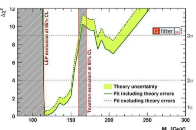
1.12 ∆χ2 _{as a function of m}

H obtained by the gFitter group by summer

2010 (before the start of LHC operations). The solid (dashed) lines corresponds to the results when including (ignoring) the theoretical

errors [19]. . . 23

1.13 The main SM Higgs boson production modes in hadron collisions. The gluon-gluon fusion (top left), the Vector boson Fusion (top right), Higgsstrahlung (bottom left) and the production in association with

top pairs (bottom right). . . 24

1.14 Cross-section of the Higgs production modes at LHC at 7 TeV (left)

and 8 TeV (right), as a function of its mass [40]. . . 25

1.15 Standard Model Higgs boson decay branching ratios as a function of

the Higgs boson mass hypothesis [40]. . . 25

1.16 Leading Feynman diagrams for the H → γγ and H → Zγ decays in

the Standard Model. . . 27

1.17 Branching fractions of Higgs decays in a fourth generation model with

md4 = ml4 = 400 GeV (right) [42]. . . 29

1.18 Enhancement in the event rate of a 115 GeV Higgs boson versus the

number of extra generations [44]. . . 29

1.19 Higgs boson decay branching ratio times the production cross section

at 7TeV in the fermiophobic Higgs model [40]. . . 31

2.1 Schematic of the accelerator system for both protons (left) and heavy

ions (right). . . 34

2.2 A Z boson event candidate decaying into a pair of muons in an

en-vironment with 25 reconstructed vertices. This event was recorded on April 15th 2012 and demonstrates the high pile-up environment in

2012 running. . . 38

2.3 Cumulative luminosity versus day delivered to ATLAS during stable

beams and for p-p collisions. This is shown for 2010 (green), 2011

(red) and 2012 (blue) running. The online luminosity is shown [68]. . 39

2.4 The peak instantaneous luminosity delivered to ATLAS per day

ver-sus time during the p-p runs of 2010, 2011 and 2012. The online

luminosity measurement is used for this plot [69]. . . 40

2.5 The luminosity-weighted distribution of the mean number of

interac-tions per bunch-crossing for the 2011 and 2012 data. This shows the full 2011 run and 2012 data taken between April 4th and November 26th. The integrated luminosities and the mean �µ� values are given

in the figure [70]. . . 40

2.6 A detailed computer-generated image of the ATLAS detector and its

subsystems [60]. . . 42

2.7 Left: Cut-away view of the ATLAS inner detector. Right: The

2.8 Average number of reconstructed primary vertices as a function of average number of pp interactions per bunch-crossing measured for the data of 2012. A second order polynomial fit is performed in the upper range of µ. For the lower values of µ, the result of mathematical

extrapolation is shown [71]. . . 44

2.9 Resolution curve extracted from ID parameters in collision data and

simulation as a function of the muon pT, for the barrel region. The

solid blue line shows determinations based on data, the dashed blue

line shows the extrapolation to pT range not accessible in this analysis

and the dashed red line shows the determinations from simulation.

The measurement is performed using 2.54 f b−1 _{of 7 TeV data [72]. . . 45}

2.10 Left: Cut-away view of the ATLAS calorimeter system [60]. . . 46

2.11 Cut-away view of an end-cap cryostat showing the positions of the three end-cap calorimeters. The outer radius of the cylindrical

cryo-stat vessel is 2.25m and the length of the cryocryo-stat is 3.17m [60]. . . . 48

2.12 RMS width of the distribution of preco

T ptrueT for jets matched to truth

jets (20 < ptrue

T < 30 GeV), before and after two pile-up

subtrac-tion methods. The RMS is presented as a funcsubtrac-tion of the number of

primary vertices (NPV) for |η| <2.4. . . 49

2.13 Resolution of x and y missing ET components as a function of the number of primary vertices for data and MC in Z → µµ candidates. The resolution after pile-up suppression, based on the ratio of the

sum pT of the tracks associated to the primary vertex and all tracks,

is also shown. . . 50

2.14 Cut-away view of the ATLAS muon system [60]. . . 51

2.15 Resolution curve extracted from MS parameters in collision data and

simulation as a function of the muon pT, for the barrel region. The

solid blue line shows determinations based on data, the dashed blue

line shows the extrapolation to pT range not accessible in this analysis

and the dashed red line shows the determinations from simulation.

The measurement is performed using 2.54 f b−1 _{of 7 TeV data [72]. . . 52}

2.16 Output and recording rates at ATLAS for the L1, L2 and EF trigger

as a function of the luminosity for a 8 TeV run [76]. . . 54

3.1 Electronics (left) and Total noise (electronics plus pile-up, right) as a

function of |η| for the different sub-systems of the LAr from data [79]. 59

3.2 Schematic view of the electrode/gap structure of the ATLAS EM

calorimeter. . . 61

3.3 Sketch of a barrel module where the different layers are clearly visible

with the ganging of electrodes in phi. The granularity in η and φ of the cells of each of the three layers and of the trigger towers is also

3.4 Layout of the signal layer for the four different types of electrodes be-fore folding. The two top electrodes (types A and B) are for the barrel and the two bottom electrodes are for the end-cap inner (left, type C) and outer (right, type D) wheels. Dimensions are in millimetres. The drawings are all at the same scale. The two or three different layers

in depth are clearly visible [60]. . . 62

3.5 Cumulative amounts of material, in units of radiation length X0 and

as a function of |η|, in front of and in the electromagnetic calorimeters. The top left-hand plot shows separately the total amount of material in front of the pre-sampler layer and in front of the accordion itself over the full η-coverage. The top right-hand plot shows the details of the crack region between the barrel and end-cap cryostats, both in terms of material in front of the active layers (including the crack scintillator) and of the total thickness of the active calorimeter. The two bottom figures show, in contrast, separately for the barrel (left) and end-cap (right), the thicknesses of each accordion layer as well as

the amount of material in front of the accordion. [60]. . . 64

3.6 Block diagram of the LAr readout electronics [60]. . . 65

3.7 Amplitude versus time for a triangular pulse of the current in a LAr

barrel electromagnetic cell and of the FEB output signal after bi-polar

shaping. Also indicated are the sampling points every 25ns [60]. . . . 66

3.8 The measured electromagnetic cluster energy as a function of the

applied high voltage. The results obtained with a barrel module (left), are shown for 245 GeV electrons (open circles), 100 GeV electrons (open diamonds) and for the 100 GeV results at the nominal voltage of 2 kV scaled to the corresponding result at 245 GeV (stars). The results obtained with an end-cap module (right) are shown for 193 GeV electrons. The curves correspond to fits with a functional form

Etot = a × Vb [60]. . . 69

3.9 _{HV distribution as a function of |η| for the EMEC. A uniform}

calorime-ter response requires a HV which varies continuously as a function of |η|, as shown by the open circles. This has been approximated by a

set of discrete values shown as full triangles [60]. . . 69

3.10 Schematic of a HV feedthrough. The value of the resistor r is 1 kΩ

and R is approximately 100 kΩ [86]. . . 72

3.11 Pair of high-voltage distribution resistors (upper) connecting the HV bus to the back sampling or directly to the middle cells by narrow copper traces. Both pictures are from a bent B electrode but

repre-sentative of all other types [82]. . . 73

3.12 Left: evolution of the resistance between ambient and LAr temper-atures. The measurements were performed while cooling down and warming up again and are normalised at room temperature. Right: ratio R(T=90 K)/R(T=300 K) and its dependence on the voltage

3.13 Left: Profile of resistance for each electrode A as a function of its iη coordinate. Right: Profile of resistance for the electrode A as a function of its iφ coordinate. These values are obtained assuming that the resistance in the back of the electrode dominate the resistance

measurement. . . 74

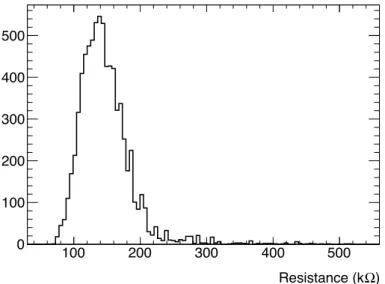
3.14 The distribution of effective resistances, integrated over iφ and iη, for

electrodes type A. . . 75

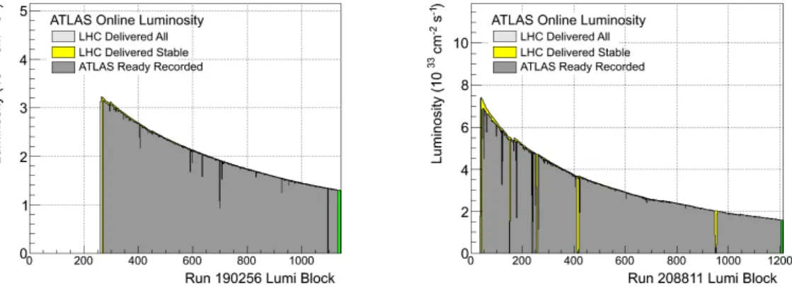
3.15 Instantaneous luminosity for chosen run in 2011 (left) and 2012 (right).These runs were selected because they span larger values of instantaneous

luminosities. . . 76

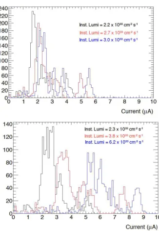
3.16 Distribution of the return currents for three values of instantaneous

luminosity for 2011 (top) and 2012 (bottom) . . . 78

3.17 Return currents of every HV line in the barrel as a function of in-stantaneous luminosity for 2011 (left) and 2012 (right). Each line represents the evolution of the return current in a HV line with the

luminosity. . . 78

3.18 The mean value of the return current of the totality of HV lines, as a

function of instantaneous luminosity for 2011 (left) and 2012 (right).. 79

3.19 The mean value of voltage drop, as a function of instantaneous

lumi-nosity for 2011 (left) and 2012 (right). . . 79

3.20 Mean value of the relative change of HV corrections as a function of

instantaneous luminosity for 2011 (left) and 2012 (right). . . 79

3.21 Currents (first column), Voltage drop (second column) and Relative change of the HV correction (third) as a function of the luminosity,

for the 9 End-Cap η regions (9 rows) in 2011. . . 81

3.22 Currents (first column), Voltage drop (second column) and Relative change of the HV correction (third) as a function of the luminosity,

for the 9 End-Cap η regions (9 rows) in 2012. . . 82

3.23 Mean value of the relative change in C’ and C’(ε) corrections as a function of the resistance variation ε, to test the sensitivity to the

resistance value, at a fixed luminosity of 6.260 ×1033_cm−2_s−1 _{in the}

barrel. . . 83

3.24 Distribution of the return currents in the barrel for the instantaneous

luminosity 5.08×1033_cm−1_s−1_{. Several sub-populations are observed:}

Region I: 0 to 3 µA. Region II: 3 to 5 µA. Region III: 5 to 6 µA. Region

IV: 6 to 8 µA. Region V: 8 to 10 µA. Region VI: 10 to 14 µA. . . 84

3.25 Return current in the barrel for the instantaneous luminosity 5.08 ×

1033_cm−1_s−1 _{as a function of its iη (left) and iφ (right) coordinates. . 84}

3.26 Return currents (first row), Voltage Drop (second row) and Relative change in the corrections (third row) as a function of the luminosity,

4.1 Display of a two silicon tracks conversion candidate.The conversion occurs on the 1st SCT layer. Both tracks have TRT extensions. The second track (on the right) has visible signs of bremsstrahlung losses as it propagates through the TRT. Both tracks show high threshold

TRT hits (3 and 11 respectively). . . 89

4.2 Overall photon reconstruction efficiencies before and after recovery as

a function of true η (top) and pT (bottom) [90]. . . 90

4.3 Expected linearity of response of the EMCAL for unconverted

pho-tons (left) and converted phopho-tons (right) as a function of

pseudo-rapidity. [94]. . . 93

4.4 Expected fractional energy resolution of the EM calorimeter for

un-converted photons (left) and un-converted photons (right) as a function

of pseudo-rapidity. [94]. . . 93

4.5 The energy-scale correction factor as a function of the pseudo-rapidity

of the electron cluster derived from fits to Z → e−_e+ _{data and. The}

uncertainties are statistical only [96]. . . 95

4.6 Electron energy response stability with µ left and with time (right)

in 2012 data [97]. . . 96

4.7 _{Reconstructed di-electron mass distributions for Z → e}−_e+ _decays

for different pseudo-rapidity regions after applying the baseline Z →

e−_e+ _{calibration. The transition region 1.37< |η| <1.52 is excluded.}

The data (full circles with statistical error bars) are compared to the signal MC expectation (filled histogram). The fits of a Breit-Wigner convolved with a Crystal Ball function are shown (full lines). The Gaussian width (σ) of the Crystal Ball function is given both for data and MC simulation. Note that the MC resolution constant term

is zero [98]. . . 97

4.8 Total systematic uncertainty on the electron energy scale (left) for the

region |η| < 0.6 which has the smallest uncertainty, and (right) for 1.52 < |η| < 1.8 which has the largest uncertainty within the central region. The uncertainty is also shown without the contribution due to

the amount of additional material in front of the EM calorimeters [74].100

4.9 Separation of direct photons vs high Et π0 shower shapes in the

EM-CAL. The narrow shower shape in the first layer correspond to a photon (left) and the structure with peaks from two close photons

coming from a π0decay [100]. . . 101

4.10 Distribution of the calorimetric discriminating variables Rη (top), Rφ

and wη for unconverted (left) and converted (right) photon candidates

with ET > 20 GeV and |η| < 2.37 (excluding 1.37 < |η| < 1.52)

selected from Z → llγ events obtained from the 2012 data sample (dots). The distributions for true photons from simulated Z → llγ events (black hollow histogram) and for fake photons from hadronic jets in Z(→ ��)+jets (red hatched histogram) are also shown. Photon isolation is required on the photon candidate but no criteria on the shower shape are applied. The photon purity of the data sample is

4.11 The mean of a binned Crystal Ball likelihood fit to the isolation dis-tribution for electrons from Z decays is shown as a function of the bunch crossing identifiers. Based calorimeter isolation is shown on

the left and in the topological isolation on the right [105]. . . 107

5.1 _{Feynman diagrams for the SM pp → Zγ productions. The top}

dia-grams a) and b) are Initial State Radiation. The bottom diadia-grams c)

and d) are Final State Radiation. . . 111

5.2 _{Candidate for a Z→ e}+_e− _{decay, with the Z boson produced in}

as-sociation with a photon, collected on 28 October 2010. The Z boson candidate invariant mass is 91 GeV. The two electrons and the photon

are well isolated. . . 112

5.3 Scatter plot of the two-body invariant mass mµµ as a function of the

three-body invariant mass mµµγ for Zγ decays in the muon channel.

The vertical pattern shows the ISR contribution with mµµ ∼ mZwhile

the horizontal pattern shows the FSR candidate where mµµγ ∼ mZ. . 112

5.4 Schema of the Double Ratio Method. The photon energy scale is ˆα,

with R(ˆα)=1. . . 115

5.5 The energy spectrum of photon candidates passing the selection in

the muon channel superimposed over the MC, shown separately for unconverted (left) and converted (right) photon candidates. The plot

contains candidates from pp data collected at √s = 7 TeV in 2011

corresponding to 4.7 fb−1_{. . . . 121}

5.6 The pseudo-rapidity distribution for photon candidates passing the

selection in the muon channel superimposed over the MC, shown sepa-rately for unconverted (left) and converted (right) photon candidates.

The plot contains candidates from pp data collected at √s = 7 TeV

in 2011 corresponding to 4.7 fb−1_{. . . . 121}

5.7 Invariant mass distribution of events passing the selection in the muon

channel superimposed over the MC, shown separately for unconverted (left) and converted (right) photon candidates. The plot contains

can-didates from pp data collected at√s = 7 TeV in 2011 corresponding

to 4.7 fb−1_{. . . . 122}

5.8 Results of the χ2 _{method : the change in χ}2 _{as a function of the}

energy scale α, for unconverted (left) and converted (right) photons. . 122

5.9 The fitted distribution of three-body mass spectrum, for selected

ra-diative FSR Z events with unconverted photons, both in data (left)

and MC (right). . . 123

5.10 The fitted distribution of three-body mass spectrum, for selected ra-diative FSR Z events with converted photons, both in data (left) and

MC (right). . . 123

5.11 The fitted distribution of two-body mass spectrum, for selected

non-radiative Z events, both in data (left) and and MC (right). . . 123

5.12 Ratio of fitted mean values as a function of α for unconverted photons

5.13 Ratios of fitted mean values without correcting the muon scale as a function of α for unconverted photons (left) and converted photons

(right). . . 125

5.14 Results of the χ2 _{method for unconverted (left) and converted (right)}

photons without correcting the muon scale. . . 125

5.15 The fitted distributions of three-body invariant mass spectrum, for selected radiative FSR Z events where the photon is unconverted. The muons are reconstructed using only the ID information. The

data sample is on the left and the MC on the right. . . 127

5.16 The fitted distributions of three-body invariant mass spectrum, for selected radiative FSR Z events where the photon is converted. The muons are reconstructed using only the ID information. The data

sample is on the left and the MC on the right. . . 127

5.17 Difference between the measured muon momentum in the MS and ID as a function of the photon energy for unconverted (left) and

con-verted (right) photons. . . 128

5.18 Photon conversion fraction in different η regions, for the electron (left)

and muon (right) channels. . . 131

5.19 Photon conversion fraction as a function of the average interactions per bunch crossing in data for the electron (left) and muon (right) channels, for total conversions (top), and one- and two-track

conver-sion (bottom). . . 131

5.20 Radius of conversion for converted photons with one and two recon-structed tracks. Photons from Z → eeγ are on the left plot, and from

Z → µµγ on the right. . . 132

5.21 The energy spectrum of photon candidates passing the selection in the electron (left) and muon (right) channels, superimposed over MC, separately shown for unconverted (top),one-track (medium) and two-track (bottom) photon candidates. The plots contain candidates from

pp data collected at √s = 8 TeV in 2012 corresponding to 20.7 fb−1_{.. 133}

5.22 Pseudo-rapidity distribution of the photon candidates passing the selection in the electron (left) and muon (right) channels superim-posed over the MC, separately shown for unconverted (top) one-track (medium) and two-track (bottom) converted photon candidates. The

plot contains candidates from pp data collected at √s = 8 TeV in

2012 corresponding to 20.7 fb−1_{. . . . 134}

5.23 Transverse momentum spectrum of the leptons passing the selection in the electron (left) and muon (right) channels superimposed over

MC. The plot contains candidates from pp data collected at √s = 8

TeV in 2012 corresponding to 20.7 fb−1_{. . . . 135}

5.24 Pseudo-rapidity distribution of the leptons passing the selection in the electron (left) and muon (right) channels superimposed over MC.

The plot contains candidates from pp data collected at √s = 8 TeV

5.25 The distributions of three-body invariant mass, for events passing the selection in the electron (left) and muon channel (right), super-imposed over the MC. The fits of a Breit-Wigner convolved with a Crystal Ball function are shown, separately for unconverted (top), one-track (medium) and two-tracks (bottom) converted photon

can-didates. . . 137

5.26 Di-lepton invariant mass distribution used for the Double Ratio method normalisation in the electron (left) and muon channel (right) super-posing data over the MC. The fits of a Breit-Wigner convolved with

a Crystal Ball function are shown. . . 138

5.27 The Double Ratio as a function of α for the three photon conversion categories extracted from the Z → eeγ (left) and Z → µµγ channel

(right). Errors are only statistical. . . 138

5.28 Fitted value of the peak mean µV (first row), resolution σCB (second

row) and wide gaussian mean value µwGA (last row) in the four pT

bins, for unconverted (left), converted one-track (middle) and

con-verted two-track (right) photons the mµµγ distribution. . . 139

5.29 Fitted value of the peak mean µV (first row), resolution σCB (second

row) and wide gaussian mean value µwGA (last row) in the four pT

bins, for unconverted (left), converted one-track (middle) and

con-verted two-track (right) photons from the meeγ distribution. . . 140

5.30 Fitted value of the peak mean µV (first row), resolution σCB (second

row) and wide gaussian mean value µwGA (last row) in the four η

bins, for unconverted (left), one-track (middle) and two-track (right)

converted photons from the mµµγ distribution. . . 141

5.31 Fitted value of the peak mean µV (first row), resolution σCB (second

row) and wide gaussian mean value µwGA (last row) in the four η

bins, for unconverted (left), one-track (middle) and two-track (right)

converted photons from the Meeγ distribution. . . 142

5.32 Fitted mean value of the Z peak µV in three different fit ranges as a

function of the photon pT for the electron (top) and muon (bottom)

channels. The fit is performed to 5000 toy datasets generated from the nominal shape extracted from data, in different mass ranges as

[60,120] (nominal), [60,130] and [70,110] GeV. . . 142

5.33 Fitted mean value of the Z peak µV in three different fit ranges as a

function of the photon |η| for the electron (top) and muon (bottom) channels. The fit is performed to 5000 toy datasets generated from the nominal shape extracted from data, in different mass ranges as

[60,120] (nominal), [60,130] and [70,110] GeV. . . 143

5.34 Photon energy scales as a function of the photon pT extracted from

the electron (left) and muon (right) channel. The scales are shown for unconverted photons (top), one-track (middle) and two-track (bot-tom) converted. The filled bands are the inclusive scale value for each category. Errors are both statistical and systematic, summed in

5.35 Photon energy scales as a function of the photon |η| extracted from the electron (left) and muon (right) channel. The scales are shown for unconverted photons (top), one-track (middle) and two-track con-verted (bottom). The filled bands are the inclusive scale value for each category. Errors are both statistical and systematic summed in

quadrature. . . 145

5.36 Combined photon energy scales as a function of the photon pT

ex-tracted from the electron and muon channel. The scales are shown for unconverted photons (top), one-track (middle) and two-track con-verted (bottom). The scales are extracted for photons calibrated with

both the in-situ Z → e+_e− _{scales and MC calibration (black filled}

cir-cles) and photons with only the MC based calibration (blue circir-cles). . 146

5.37 Combined photon energy scales as a function of the photon |η| ex-tracted from the electron and and muon channel. The scales are shown for unconverted photons (top), one-track (middle) and two-track converted (bottom). The scales are extracted for photons

cal-ibrated with both the in-situ Z → e+_e− _{scales and MC calibration}

(black filled circles) and photons with only the MC based calibration

(blue circles). . . 147

6.1 _{The di-photon mass distribution for H → γγ signal events, for}

dif-ferent algorithms used to determine the longitudinal vertex position of the event. The use of calorimeter information, labelled as “Calo pointing” is fully adequate to reach the optimal achievable mass reso-lution labelled as “True vertex”. The likelihood described in the text, combining with tracking information, provides similar mass

resolu-tion [117]. . . 156

6.2 Reconstructed inclusive invariant mass distribution for a simulated

signal of mH=125 GeV in MC12 for which a smearing has been

ap-plied to the photons energy, to account for differences in the Z → ee mass resolutions between data and MC. The result of the fit is

su-perimposed. The core component of the mass resolution, σCB, is 1.64

GeV and the FWHM of the distribution is 3.94 GeV. . . 156

6.3 _{Relative fraction of the three conversion categories for a H → γγ}

sample with a mH of 120 GeV with MC10 reconstruction. . . 158

6.4 The values of the signal PDF parameters, fitted to invariant mass

distributions of the Higgs signal with mass of 120 GeV (with MC10 reconstruction), for nine categories based on the conversion status of each photon. In the upper figure the fitted mean value of the Crystal

ball (µCB) is shown, in the middle the resolution (σCB) and in the

bottom the tail parameter αCB. . . 159

6.5 Illustrative plot of the gaussian fit in an asymmetric restricted range

between -1.5σ and +2.0σ to the ∆ distribution (see Equation 6.2). The ∆ distribution corresponds to unconverted photons with 20 GeV<

6.6 The fitted mean value of the ∆ distribution, as a function of the

photon pT, for different η regions of the detector. The distribution is

fitted to a gaussian in a restricted range. . . 162

6.7 Mean value of the Rφ distribution in pT and η bins for the three

types of photon conversion categories, unconverted (top), one-track

converted (middle), two-track converted(bottom). . . 163

6.8 Schema of sources of mis-calibration in converted photons. Two

ef-fects are shown, the front energy loss and the out of cluster effect. . . 164

6.9 Fitted mean value of the ∆ distribution corrected by the converted

photon calibration tool, as a function of the photon pT, for different

η regions of the detector. The distribution is fitted to a gaussian in a

restricted range. . . 165

6.10 Invariant mass PDF of the H→ γγ signal in MC11 with (red) and without (black) the converted photon energy correction. The signal for pairs of one-track converted photons (left) and two-track converted

photons (right) is shown. . . 167

6.11 Correlation matrix (left) and global correlations (right) of the 7 free parameters in the resolution model R of a Crystal Ball and a wide

Gaussian fitted on a MC11 sample with mH = 125 GeV. . . 168

6.12 Reconstructed invariant mass distributions for hypothesised Higgs

masses of mH =100 GeV, mH =120 GeV and mH =140 GeV with

MC11. . . 169

6.13 Signal PDFs extracted from a MC11 ggF sample with mH = 125 GeV

for shapes using different values of the tail parameter nCB. . . 170

6.14 Signal PDFs extracted from a MC11 ggF sample with mH = 125

GeV for different hypotheses of the µGA parameter. In one case the

mean value of the gaussian is unconstrained, and in a second case it

is forced to be equal to the mean value of the Crystal Ball. . . 170

6.15 Reconstructed invariant mass distributions from the signal processes and the projection of the global fit in all available MC mass points at 8 TeV. In the figures, the plotted invariant mass increases from 100 GeV to 150 GeV in 5 GeV steps. The parameters appearing in the

figures are the evaluation of the global function at that mass point. . 172

6.16 Reconstructed invariant mass distributions and the projection of the global fit at 120 GeV for the signal processes ggF, VBF, WH, ZH and

ttH at 8 TeV. . . 173

6.17 Expected SM signal yields parametrisation as a function of the mγγ

mass. The yields corresponds to the prediction at 1 f b−1 _{of 8 TeV}

data in the inclusive category. . . 175

6.18 Sketch of the pTt definition. . . 177

6.19 Distribution of pTt in simulated events with Higgs boson production

and in background events. The signal distribution is shown sepa-rately for gluon fusion (blue), and vector-boson fusion together with associated production (red). The background MC and the two signal

6.20 Reconstructed invariant mass distributions from the signal processes and the projection of the global fit at the MC 125 GeV mass point at 7 TeV for all categories. The parameters appearing in the figures are the evaluation of the global function at that mass point for each

category. . . 182

6.21 Reconstructed invariant mass distributions from the signal processes and the projection of the global fit at the MC 125 GeV mass point at 8 TeV for all categories. The parameters appearing in the figures are the evaluation of the global function at that mass point for each

category. . . 183

6.22 Invariant mass distributions for a Higgs boson with a hypothesised

mass of 125 GeV, for the best-resolution category (σCB=1.4 GeV)

shown in blue and for a category with lower resolution (σCB=1.9

GeV). . . 185

6.23 Background-only fits to the di-photon invariant mass spectra for the ten categories. The bottom inset displays the residual of the data with respect to the background fit. The Higgs boson expectation for a mass hypothesis of 126.5 GeV corresponding to the SM cross-section

is also shown. All figures correspond to the√s = 7 TeV data sample [3].187

6.24 Background-only fits to the di-photon invariant mass spectra for the ten categories. The bottom inset displays the residual of the data with respect to the background fit. The Higgs boson expectation for a mass hypothesis of 126.5 GeV corresponding to the SM cross-section

is also shown. All figures correspond to the√s = 8 TeV data sample [3].188

6.25 Invariant mass distribution of di-photon candidates for the combined 7 TeV and 8 TeV data samples. The result of a fit to the data of the sum of a signal component fixed to an hypothesised Higgs mass of 126.5 GeV and a background component described by a fourth-order Bernstein polynomial is superimposed. The bottom inset displays the residuals of the data with respect to the fitted background

com-ponent [3]. . . 190

6.26 Expected and observed CLs limit on the normalised signal strength

as a function of the assumed Higgs boson mass for the combined √s

= 7TeV and√s = 8TeV analysis. The dark (green) and light (yellow)

bands indicate the expected limits within ± 1 sigma and ± 2 sigma

fluctuations, respectively [3]. . . 194

6.27 Expected and observed local p0 values for a SM Higgs boson as a

function of the hypothesised Higgs boson mass (mH) for the combined analysis and for the 7 TeV and 8 TeV data samples separately. The observed p0 including the effect of the photon energy scale uncertainty on the mass position is included via pseudo-experiments and shown

as open circles [3]. . . 195

6.28 Best fit value for the signal strength as a function of the assumed

6.29 Best fit value for the signal strength for the different categories at

a Higgs mass of 126 GeV for the for the combined √s = 7TeV and

√_{s = 8TeV data samples. The band corresponds to the error of the}

combined result [3]. . . 196

6.30 Confidence intervals contours for the H to gamma gamma channel

in the (µ, mH) plane. The 68% and 95% CL contours are for the

combined 7 TeV and 8 TeV analysis. The light lines indicate the effect of holding constant at their best-fit values the nuisance parameters which describe the energy scale systematic (ESS) uncertainties in the

likelihood [3]. . . 197

6.31 Invariant mass distribution of di-photon candidates for the combined 7 TeV and 8 TeV data samples. The result of a fit to the data of the sum of a signal component fixed to an hypothesised Higgs mass of 126.8 GeV and a background component described by a fourth-order Bernstein polynomial is superimposed. The bottom inset displays the residuals of the data with respect to the fitted background

com-ponent [55]. . . 198

6.32 The observed local p0 value as a function of mH for the TeV data

(blue), 8 TeV data (red), and their combination (black). The

ex-pected local p0 under the SM Higgs boson signal plus background

hypothesis is shown in dashed curves. The largest local significance in the combination of 7 TeV data and 8TeV data is found to be 7.4σ

at mH =126.5GeV, where the expected significance is 4.1σ [55]. . . . 198

6.33 Confidence intervals contours for the H to gamma gamma channel in

the (µ, mH) plane. The 68% and 95% CL contours are for the

com-bined root √s = 7TeV and root√s = 8TeV analysis. Results when

photon energy scale systematic uncertainties are removed (dashed), and results when all systematic uncertainties are removed (dotted),

are also shown [55]. . . 199

6.34 Expected distributions of likelihood ratio, for the combination of channels as a function of the fraction of the spin-2 production mecha-nism. The green and yellow bands represent, respectively, the one and

two standard deviation bands for the 0+ (a) and for the 2+ (b) [134]. 200

6.35 Top: The measured production strengths for a Higgs boson of mass

mH =125.5 GeV, normalised to the SM expectations, for diboson

fi-nal states and their combination. The best-fit values are shown by the solid vertical lines. The total ±1σ uncertainty is indicated by the shaded band, with the individual contributions from the statistical uncertainty (top), the total (experimental and theoretical) system-atic (middle), and the theory uncertainty (bottom) on the signal cross section (from QCD scale, PDF, and branching ratios) shown as super-imposed error bars. Bottom: Measured signal strengths, normalised to the SM expectation, for the three individual production mecha-nisms and for a Higgs boson mass of 126.8 GeV. The last line shows the result for a global strength parameter µ applied to all produc-tion modes. The error bars indicate the total uncertainty (black), the

7.1 Photon pT (left) and η (right) for signal (ggF with mH = 125 GeV)

and background (SM Zγ) events. MC11 samples are used. . . 209

7.2 Three-body invariant mass distribution for SM Zγ background for

different cuts on the photon pT. MC11 is used. . . 210

7.3 Fitted mean value of the background shape as a function of the photon

pT cut. . . 211

7.4 Scatter plot of the m(��) m(��γ) masses for a Higgs signal with mH =

125 GeV, for the electron channel. MC12 samples are used. . . 212

7.5 Scatter plot of the m(��) m(��γ) masses for a Higgs signal with mH =

125 GeV, for the muon channel. MC12 samples are used. . . 212

7.6 Reconstructed invariant mass distributions from the signal processes

for each one of the resolution improvements. Red: Invariant mass distribution without improvements, Blue: Invariant mass distribution correcting the photon position by the primary vertex and the Z mass constraint. Left is the distribution for electrons, right for muons in

MC samples at 8 TeV. . . 214

7.7 Reconstructed ∆m distributions from the signal processes for each one

of the resolution improvements. Red:∆m distribution only correcting the photon position by the primary vertex. Blue: ∆m distribution correcting the photon position by the primary vertex and the Z mass constraint. Left is the distribution for electrons, right for muons in

MC samples at 8 TeV. . . 214

7.8 Signal efficiency for events produced in pp collisions at √s = 7 TeV.

Top row: signal selection efficiency versus nominal Higgs mass for gluon fusion (left) and VBF (right) events, when the Z boson decays

to e+_e−_{. Bottom row: signal selection efficiency versus nominal Higgs}

mass for gluon fusion (left) and VBF (right) events, when the Z boson

decays to µ+_µ−_{. . . . 215}

7.9 Signal efficiency for events produced in pp collisions at √s = 8 TeV.

Top row: signal selection efficiency versus nominal Higgs mass for gluon fusion (left) and VBF (right) events, when the Z boson decays

to e+_e−_{. Bottom row: signal selection efficiency versus nominal Higgs}

mass for gluon fusion (left) and VBF (right) events, when the Z boson

decays to µ+_µ−_{. . . . 217}

7.10 Distribution (normalised to unit area) of the difference ∆m between

the final state three-body invariant mass m��γ and the di-lepton

in-variant mass m�� for signal events passing the full selection (dots), for

mH = 125 GeV and √s = 7 (top) or 8 (bottom) TeV. The line

over-laid represents the projection of a global fit on the distribution with a model composed of the sum of a Crystal Ball (CB) and a Gaussian

7.11 Background-only fits to the distribution of the mass difference ∆m of selected events in data, for Z → ee (left) and Z → µµ (right), at

√_{s = 7 TeV (top) or 8 TeV (bottom). For both 7 and 8 TeV, a third}

order polynomial is used for the fit. Dots correspond to data, the blue line is the fit result and the gray and light red bands are the 1σ and 2σ uncertainty bands from the statistical uncertainties on the fitted background model parameters. The dashed histograms correspond to the SM signal expectation, for a Higgs boson mass of 125 GeV, scaled

by a factor 20 for clarity [4]. . . 221

7.12 Observed 95% CL limits (solid black line) on the production cross section of a SM Higgs boson decaying to Zγ, as a function of the

Higgs boson mass, using 4.6 fb−1 _{of pp collisions at} √_{s = 7 TeV and}

20.7 fb−1 _{of pp collisions at} √_{s = 8 TeV. The median expected 95%}

CL exclusion limits (dashed red line) are also shown. The green and

2.1 Parameters of the LHC proton-proton collisions for the data-taking periods: 2010, 2011 and 2012, and the design values. The quoted

parameters are: the center-of-mass energy √s, the number of

pro-tons per bunch Nb, the number of bunches per beam nb and the

bunch-to-bunch time spacing ∆t. Each value corresponds to the best

performance achieved during the year [65, 66]. . . 35

2.2 Effective constant term measurements from data (from the observed

width of the Z → e+_e−_{peak), for different subsystems of the EMCAL:}

Barrel, End-Cap (Inner Wheal and Outer Wheal), and the forward

calorimeter [74, 75]. . . 47

3.1 Detector-oriented coordinates iη and iφ in the barrel and their range

in each region of the electrode.. . . 71

3.2 _{The effective resistances of HV line, for the nine |η| regions in the}

End-Cap. . . 75

3.3 Operational Voltage for 10 η regions in the EMCAL. . . 77

3.4 Relative change in the HV corrections for various end-cap regions in

2012. . . 80

3.5 Summary of results : HV corrections and voltage drops, for various

eta regions. . . 86

5.1 Selection criteria applied on muon candidates, for the 2011 and 2012

analyses. . . 119

5.2 Selection criteria applied on electron candidates, for the 2011 and

2012 analyses. . . 120

5.3 Selection criteria applied on photon candidates, for the 2011 and 2012

analyses. . . 120

5.4 Details about the selection of Z events, including FSR events in 2011

and 2012 analyses. . . 120

5.5 _{Photon scales for the two channels Z → µµγ and Z → eeγ.} . . . 125

5.6 Selected events in data and MC for the 8 TeV analysis. . . 130

5.7 Combined scales for fully calibrated photons in different pT bin for all

conversion categories. The scales are in percentage. . . 148

5.8 Combined scales for fully calibrated photons in different η bin for all

conversion categories.The scales are in percentage. . . 149

6.1 Description of categorisation by photon conversion status. The first digit in the category nomenclature corresponds to the conversion

sta-tus of the leading photon, and the second to the sub-leading photon.. 157

6.2 Fitted parameters of the signal PDF for two cases: Invariant mass

built with pairs of one-track converted photons and pairs of two-track converted photons. The change between the parameters after

implementing the correction is presented. . . 166

6.3 Expected Higgs boson signal efficiency ε (including acceptance of

kine-matic selections as well as photon identification and isolation efficien-cies) and event yield for H → γγ assuming an integrated luminosity of

4.8 fb−1 for the √s =7 TeV data (top) and of 5.9 fb−1 for the √s = 8

TeV data (bottom). Results are given for different production

pro-cesses and in 5 GeV mH steps. . . 179

6.4 Number of expected signal events per category at mH = 126.5 GeV,

at √s = 7 TeV (top) and √s = 8TeV (bottom) and breakdown by

production process. . . 180

6.5 The numerical results of the global fit. The linear dependence of the

µCB shape parameter is given by µCB(M ) = M − 125 + µ(125) + ∆µ×

(M − 125); and similarly for the σCB. The outlier mean value µGA is

set to µGA = µCB, and the width of the outlier component is set to

σGA = κGA× σCB with a single value for κGA. Parameters with (*)

are fixed in the fit, therefore no statistical errors. . . 184

6.6 Systematic uncertainties in the number of signal events fitted due to

the background parametrisation, given in number of events. Three different background parametrisation are used depending on the cat-egory, an exponential function, a fourth-order Bernstein polynomial

and the exponential of a second-order polynomial [117]. . . 186

6.7 Number of expected signal S and background events B in mass a

window around mH = 126.5 GeV that would contain 90% of the

expected signal events. In addition, σCB, the Gaussian width of the

Crystal Ball function describing the invariant mass distribution [117], and the FWHM of the distribution, are given. The numbers are given

for data and simulation at √s = 7 TeV (top) and 8 TeV (bottom)

for different categories and the inclusive sample. . . 189

7.1 Trigger used to selected data, for the 2011 and 2012 analyses. . . 207

7.2 Selection criteria applied on muon candidates, for the 2011 and 2012

analyses. Combined muons are referred as “CB”, Stand-alone muons

as “StandA.” and Calo muons as “Calo”. . . 208

7.3 Selection criteria applied on electron candidates, for the 2011 and

2012 analyses. . . 208

7.4 Selection criteria applied on photon candidates, for the 2011 and 2012

analyses. . . 209

7.5 Details about the selection of Higgs events, in the 2011 and 2012

analyses. . . 209

7.7 Number of expected signal events in the muon channel for each pro-duction process and Higgs boson masses in 5 GeV steps between 110

and 150 GeV, for 4.6 fb−1_{, at} √_{s = 7 T eV . . . . 216}

7.8 Number of expected signal events in the electron channel for each

production process and Higgs boson masses in 5 GeV steps between

110 and 150 GeV, for 4.6 fb−1_{, at} √_{s = 7 T eV . . . . 216}

7.9 Number of expected signal events in the muon channel for each

pro-duction process and Higgs boson masses in 5 GeV steps between 110

and 150 GeV, for 20.7 fb−1_{, at} √_{s = 8 T eV . . . . 216}

7.10 Number of expected signal events in the electron channel for each production process and Higgs boson masses in 5 GeV steps between

110 and 150 GeV, for 20.7 fb−1_{, at} √_{s = 8 T eV . . . . 217}

7.11 The numerical results of the global fit. The linear dependence of the

µCB shape parameter is given by dµCB(∆m) = ∆m + dµ(∆m125) +

∆µ×(∆m−∆m125); and similarly for the σCBshape parameter with

∆m125 = (125 − MZ) GeV. The width of the outlier component is

set to σGA = κGA × σCB with a single value for κGA. . . 219

7.12 Theoretical systematic uncertainties for the SM Higgs boson produc-tion cross secproduc-tion and branching fracproduc-tion of the H → Zγ decay at √

s = 7 and 8 TeV, for a Higgs boson mass of 125 GeV [4]. . . 222

7.13 Summary of the systematic uncertainties on the signal yield and

The Standard Model (SM) of particle physics, provides a nearly complete view of the elementary composition of matter and the electromagnetic, weak and strong forces, which are the three dominant interactions at subatomic level. Built over the last half of the 20th century, the SM has successfully explained most experimental results and precisely predicted a wide variety of phenomena.

One important piece of the SM is the mechanism responsible for the electroweak symmetry breaking (EWSB) which provides masses to the vector bosons W± _{and Z}

and the fermions. This mechanism predicts the existence of a particle, the so-called Higgs boson. For many years, experiments from colliders such as LEP and Tevatron searched for the Higgs boson without finding any direct strong evidence to confirm the theory. This scenario changed after the first run of the Large Hadron Collider (LHC).

The LHC is the largest and most powerful particle accelerator ever built. Its operations started up in the year 2010, when the first proton-proton collisions with a centre-of-mass energy of √s = 7 TeV and instantaneous luminosities up to 1032_cm−2_s−1 _{were recorded, setting the beginning of a new era in high energy}

physics experiments. The LHC ran for three years, initially at√s = 7 TeV in 2010-2011 and at √s = 8 TeV in 2012 and delivered proton-proton (and also heavy ions) collisions to four main experiments. The ATLAS detector is one of the two general purpose experiments, with an extensive physics program including the search for the SM Higgs boson and the search for new physics. By the end of the first run of the LHC, the elusive Higgs boson was finally observed, and some of its properties measured.

This thesis presents both detector oriented studies and physics analyses concerning photons. The first part of the document contains detector and performance anal-yses, where a study on the high-voltage system of the electromagnetic calorimeter

(EMCAL) is performed. Furthermore, photon performance studies are presented, where the standard calibration of the EMCAL is validated using radiative Z decays. Concerning physics analyses, the results of the searches for the Higgs Boson in the γγ and Zγ decay channels in ATLAS are presented, using 4.8 fb−1 _{of data recorded}

at √s = 7 TeV and 5.9/20.7 fb−1 _at √_{s = 8 TeV in the γγ and Zγ channels,}

re-spectively. The main motivation of studying simultaneously these channels is that in the SM, both decays are mediated via top and W loops. These two channels are therefore sensitive to new physics, as any deviation of these decays rates with respect to the SM may occur via contributions from new heavy charged particles.

Outline

In Chapter 1, a brief introduction on the theoretical framework of the SM and Higgs phenomenology is presented. Chapter 2 describes the LHC complex at CERN and the ATLAS detector. In Chapter3, a detailed description of the EMCAL, including studies performed in the high-voltage system are exposed. Chapter 4 describes the standard reconstruction, identification and calibration of photons in ATLAS. A data-driven method to validate the standard EMCAL in-situ calibration using Z radiative decays is presented in Chapter 5. Chapter 6 describes the search for the SM Higgs boson decaying into a photon pair, the content of this chapter includes preliminary MonteCarlo-based signal studies and the analysis which lead to the observation a Higgs boson-like particle with a mass of about 126.5 GeV. Finally, in Chapter 7, the first ATLAS result in the search for the SM Higgs boson in the Zγ decay channel is presented.

Personal Contributions

Research in experimental high energy physics relies heavily on collaboration. There-fore, the work presented in this thesis is the result of contributions made by many people working on different areas. Leading personal contributions of various analyses presented in this thesis, divided by chapter, are presented below.

Chapter 3: High-Voltage studies. A study on the effect of resistors in the electrodes of the EMCAL on the high-voltage system and on the energy measurement is presented. This study is documented in [1].

Chapter 5: Photon energy scales. A data-driven validation to the standard calibration is performed extracting the photon energy scales from a sample of Z radiative decays. The analysis is performed using both 7 and 8 TeV data. The results presented in this thesis at 7 TeV are obtained in collaboration with the ATLAS Tokyo group. The complete 8 TeV results correspond to personal contributions. The 7 TeV results can be found in [2], and documentation for the results at 8 TeV is in the final stages of editing.

Chapter 6_{: Signal studies for the H → γγ channel. A number of studies}

were performed to investigate the photon performance in the MC and to improve the signal model used in the final statistical analysis. An analytical signal resolution model is built to satisfy the need for an interpolation of the signal invariant mass probability density function for the search. The global signal resolution model is used in the discovery analysis, and plays an important role in the mass measurement in this channel. This contribution appears in [3].

Chapter 7_{: Search for the SM Higgs boson in the H → Zγ channel.}

Personal contributions at several levels of the analysis are presented, which includes the choice of the discriminanting variable for the search, optimisations of the photon selection, background parametrization studies and the signal modelling for the final result. These contributions are documented in [4, 5].

The Standard Model of Particle

Physics and the Higgs boson

Contents

1.1 Gauge symmetries in Quantum Electrodynamics . . . . 8

1.2 Basics of Quantum Chromodynamics . . . 10

1.3 Electroweak theory and the Higgs mechanism . . . 11

1.3.1 Electroweak theory . . . 11

1.3.2 The Higgs Mechanism . . . 12

1.3.3 The SM Higgs boson . . . 13

1.4 Constraints in the SM Higgs mass . . . 15

1.4.1 Theoretical Constraints . . . 15

1.4.2 Experimental constraints before the LHC . . . 20

1.5 The SM Higgs boson at the LHC . . . 23

1.5.1 The Higgs production . . . 23

1.5.2 The Higgs decay modes . . . 24

1.6 The _{H → γγ and H → Zγ channels} . . . 26

1.7 Beyond the SM. . . 27

1.7.1 Fourth Generation Model of Quarks and Leptons . . . 28

1.7.2 Models with Higgs extensions . . . 28

1.7.3 Fermiophobic Higgs boson . . . 30

1.8 Results from the first run of the LHC Run . . . 30 5