Combining Heuristics to Optimize and Scale the Placement of IoT Applications in the Fog

HAL Id: hal-01942097

https://hal.inria.fr/hal-01942097

Submitted on 2 Dec 2018

HAL is a multi-disciplinary open access

archive for the deposit and dissemination of

sci-entific research documents, whether they are

pub-lished or not. The documents may come from

teaching and research institutions in France or

abroad, or from public or private research centers.

L’archive ouverte pluridisciplinaire HAL, est

destinée au dépôt et à la diffusion de documents

scientifiques de niveau recherche, publiés ou non,

émanant des établissements d’enseignement et de

recherche français ou étrangers, des laboratoires

publics ou privés.

Combining Heuristics to Optimize and Scale the

Placement of IoT Applications in the Fog

Ye Xia, Xavier Etchevers, Loic Letondeur, Adrien Lebre, Thierry Coupaye,

Frédéric Desprez

To cite this version:

Ye Xia, Xavier Etchevers, Loic Letondeur, Adrien Lebre, Thierry Coupaye, et al..

Combining

Heuristics to Optimize and Scale the Placement of IoT Applications in the Fog. UCC 2018 : 11th

IEEE/ACM Conference on Utility and Cloud Computing, Dec 2018, Zurich, Switzerland. pp.1-11,

�10.1109/UCC.2018.00024�. �hal-01942097�

Combining Heuristics to Optimize and Scale

the Placement of IoT Applications in the Fog

Ye Xia

Meylan, France ye.xia@orange.com

Adrien Lebre

Nantes, France adrien.lebre@inria.fr

Xavier Etchevers

Thierry Coupaye

Lo¨ıc Letondeur

Fr´ed´eric Desprez

Grenoble, France frederic.desprez@inria.fr

Abstract—As fog computing brings processing and stor-age resources to the edge of the network, there is an in-creasing need of automated placement (i.e., host selection) to deploy distributed applications. Such a placement must conform to applications’ resource requirements in a het-erogeneous fog infrastructure, and deal with the complex-ity brought by Internet of Things (IoT) applications tied to sensors and actuators. This paper presents four heuristics to address the problem of placing distributed IoT appli-cations in the fog. By combining proposed heuristics, our approach is able to deal with large scale problems, and to efficiently make placement decisions fitting the objective: minimizing placed applications’ average response time. The proposed approach is validated through comparative simulation of different heuristic combinations with varying sizes of infrastructures and applications.

Index Terms—placement, heuristics, fog computing, IoT

I. INTRODUCTION

After a decade of continuous growth of cloud com-puting, which concentrates processing and storage re-sources for hosting on-demand enterprise and web ap-plications, we can now witness the emergence of more distributed paradigms, such as fog computing [1], [2]. Motivated by Internet of Things (IoT) applications that require low response times, data privacy enforcement, and the control over the amount of data commuting by the core network, fog computing makes use of devices in the edge of the network, and provides processing, storage, and network resources close to sensors and actuators. To take advantages of local resources pro-vided by the fog, a proper decision of where to place distributed applications (i.e., how to select applications’ hosts) must be made. Such placement decisions impact both applications’ performance and hardware resource consumption. However, known to be an NP-hard prob-lem [3], [4], applications’ placement decision-making in the context of IoT and fog exhibits the following challenges:

• Heterogeneity: a fog infrastructure contains a large number of heterogeneous devices connected to var-ious networks. These devices’ resource capacities,

network positions, and privacy / hardware / software features strongly differ.

• Constraint diversity: to be executed properly, IoT applications must conform to many kinds of con-straints, which can be related to consumable re-sources (e.g., processing and bandwidth capacities), non-consumable properties (e.g., network latency, privacy), and different entities (e.g., software ele-ments and communication channels composing ap-plications).

• Locality and geo-distribution: as sensors / actuators are spread over different geographical locations, an IoT application, which is by definition tied to sensors / actuators, can span multiple localization areas. • Scalability: to be reactive to applications’

deploy-ment requests, placedeploy-ment decisions must be made time-efficiently. However, the complexity of the placement problem dramatically increases with the infrastructure’s and applications’ sizes, which makes it hard to deal with large-scale problems.

This work proposes a set of heuristics to overcome aforementioned challenges. In particular, the combi-nation of proposed heuristics highly improve: i) the placement algorithm’s scalability by accelerating the placement decision-making process; ii) the placement result quality by better fitting the objective—minimizing applications’ response times. Leveraging our previous work [5] (more details are given in Section II), this paper makes the following contributions:

• Four heuristics that can be combined to each other. Compared with [5], heuristics proposed in this work allow the placement approach to deal with even larger problems and to make placement decisions leading to even lower response times.

• A simulation-based evaluation that compares different heuristic combinations from two aspects: i) scalability in terms of the problem scale that an algorithm can deal with within a timeout; ii) result quality in terms of placed applications’ average response time.

The rest of this paper is organized as follows. Section II reminds our previous work [5]’s proposal. Section III proposes new heuristics. These heuristics are evaluated in Section IV. Section V discusses re-lated works.Section VIconcludes and discusses future works.

II. BACKGROUND

This section reminds the model, the naive placement algorithm, and heuristics proposed in [5].

A. Model and Problem Formulation

A fog infrastructure contains two kinds of devices: i) fog nodes (e.g., cloud, edge server), which provide processing and storage resources; ii) appliances (e.g., sensor, actuator), which provide sensing / actuating services. Only fog nodes can be used as hosting devices. Appliances do not provide resources to host applica-tions. A fog infrastructure also consists of links, which connect devices and provide network resources.

An IoT application is composed of components, bindings, and appliances1_{. A component is a software}

element that can be executed on one fog node. A binding is a communication channel that connects a couple of components or a component and an appliance.

Inf ra a fog infrastructure

nodei a fog node of Inf ra

nodei.CP U nodei’s available CPU capacity

nodei.RAM nodei’s available RAM capacity

nodei.DISK nodei’s available DISK capacity

appliancei an appliance of Inf ra

linki a link of Inf ra

linki.LAT linki’s network latency

linki.BW linki’s available bandwidth capacity

Apps a set of applications to place

compi a component of an application in Apps

compi.ReqCP U compi’s CPU requirement

compi.ReqRAM compi’s RAM requirement

compi.ReqDISK compi’s DISK requirement

compi.DZ compi’s Dedicated Zone

bindi a binding of an application in Apps

bindi.ReqLAT bindi’s latency requirement

bindi.ReqBW bindi’s bandwidth requirement

appi an application in Apps

appi.components all components of appi

appi.appliances all appliances of appi

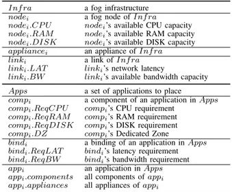
Table I: Summary of Notations.

As summarized in Table I, this work’s model char-acterizes each component comp with: i) ReqCP U , ReqRAM , and ReqDISK, which respectively indicate CPU, RAM, and DISK capacities that comp needs; ii) a Dedicated Zone (DZ), which is a deployment area composed of a set of fog nodes respecting comp’s requirements on fog node properties (e.g., privacy, OS, etc). Bindings are characterized with requirements as well. bindi.ReqBW designates bindi’s bandwidth

re-quirement. bindi.ReqLAT indicates the maximal

net-work latency that bindi can accept.

1_{As a sensing / actuating service must be executed on its appliance,}

we do not differentiate an appliance with its service.

A placement maps each component onto a fog node. A solution to a problem is a placement that satisfies the following constraints: i) each component is placed in its DZ; ii) required CPU, RAM, and DISK in each fog node do not exceed the fog node’s capacities; iii) required bandwidth in each link does not exceed the link’s capacity; iv) each binding’s latency does not exceed the binding’s requirement.

A placement problem can have multiple solutions, among which only one can be selected as the placement decision. To fit the objective of minimizing considered applications’ response times2_{, the following objective}

function is applied: min: W AL = ∑ bind ∈ Apps bind.ReqBW total BW × bind.Lat total BW= ∑ bind ∈ Apps bind.ReqBW

total BW is the total bandwidth requirement of all bindings. bind.Lat is bind’s latency regarding the eval-uated solution3. The objective function is to minimize

Weighted Average Latency (WAL) of Apps. Consider-ing that a bindConsider-ing with a high ReqBW can strongly impact an application’s response time, each binding’s latency is weighted by a proportion of its ReqBW regarding total BW . Through minimizing WAL, la-tencies of bindings, especially of the bindings with high ReqBW s, are minimized, which helps to decrease applications’ response times. Ideally, given a placement problem, the solution with minimal WAL should be selected as the placement decision.

B. FirstFit Backtrack Search

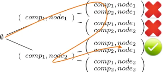
Based on depth-first search, a FirstFit backtrack al-gorithm is implemented to find solutions. As named, FirstFit returns the first solution found. It deals with a set of applications: components of all considered applications are mixed and placed one by one. When FirstFit tries to place a component comp, all kinds of constraints are verified for comp and components al-ready placed. As depicted inFigure 1, when a constraint verification is passed, FirstFit continues with the next component. Once all the components are successfully placed, it implies that a solution is found. If a constraint verification fails, FirstFit tests the next fog node to place comp. If all possible fog nodes are tested, and no suitable fog node is found, FirstFit backtracks to the previous component and changes its host. When FirstFit backtracks from the first component, it implies that the search space has been traversed, and no solution

2_{The response time is composed of communication time (i.e., time}

spent to transfer messages) and execution time (i.e., time spent within components for processing). With processing resource requirements predefined for each component, the execution time is assumed to change insignificantly with placement, and this work tries to minimize only the communication time.

3_{Given a solution in which each component is placed in a fog node,}

each binding must be correspondingly placed in a communication path composed of a set of links. A binding’s latency is the network latency of its communication path.

exists. By continuing the search until a solution is found, FirstFit guarantees to find a solution, if any exists.

∅ ( comp1, node2 ) ₍ comp1, node2 comp2, node2 ) ( comp1, node2 comp2, node1 ) ( comp1, node1 ) ₍ comp1, node1 comp2, node2 ) ( comp1, node1 comp2, node1 )

Figure 1:FirstFit Search Process Example (FirstFit begins by testing to place comp1 in node1, which passes; then it fails

to place comp2 in node1 and node2 because of constraint

violations; having tested all possible fog nodes for comp2,

FirstFit backtracks to comp1and continues the search; finally,

it returns the first solution found, in which comp1and comp2

are respectively placed in node2 and node1.).

A number of tests must be carried out before FirstFit returns (e.g., there are five tests inFigure 1). To reduce the number of tests (i.e., to accelerate the search), when trying to place a component comp, fog nodes out of comp’s DZ are not tested (because a component must be placed in its DZ).

FirstFit has no guarantee on WAL values of returned solutions or needed numbers of tests, which can incur low result quality and high execution times.

C. Previously Proposed Heuristics

To overcome FirstFit’s drawbacks, two heuristics have been proposed in [5], which respectively manip-ulate two test orders of FirstFit: fog nodes’ order and components’ order.

The heuristic Anchor-based Fog Nodes Ordering (AFNO) calculates each component’s anchor (i.e., the fog node that best localizes4 the component in terms of minimizing WAL) with an iterative algorithm. With fewer constraints taken into account (i.e., constraints ii, iii, and iv stated in Section II-A are not considered), anchors’ calculation has a lower complexity than the placement problem. Before testing fog nodes to place a component comp, AFNO sorts fog nodes in ascending order of network latency to comp’s anchor. Therefore, the first solution found must be close to the anchors and thus helps to minimize WAL. Moreover, by minimizing WAL, anchors help to minimize bindings’ latencies, which makes bindings’ requirements on maximal la-tency prone to be satisfied. Thus, AFNO also guides components to network positions close to a solution, and thereby accelerates the search.

The other heuristic, Dynamic Components Ordering (DCO(1), more details are given in Section III-B), dynamically adjusts components’ order to accelerate the search. When FirstFit fails to place a component comp and backtracks, because changing any placed compo-nent’s host to any fog node is possible to solve the

4_{The verb “localize” differs with “place” on constraints taken into}

account. To localize a component considers only constraint i (i.e., placing each component in its DZ) stated inSection II-A, while to place a component must take all the constraints into account.

failure of placing comp, FirstFit tests all the possibilities one by one in a random manner, which can lead to a huge amount of tests. To avoid such cases, instead of backtracking, DCO(1) set comp as the first component to place (hence, no other component can constrain it), and redoes the search all over again under the new component order.

Although these two heuristics highly improve First-Fit according to [5]’s evaluation, they can be further enhanced. Regarding anchor’s definition, a component comp’s anchor depends on locations of components that comp communicates with. When AFNO calculates comp’s anchor, other components are considered to be located on their anchors. However, during the search, in which all constraints must be taken into account, a component’s host can be different from its anchor, which can make other anchors outdated. With outdated anchors, the search is no longer guided properly. For DCO(1), after reordering a component to the head, all the hosts found under the previous component order can not be reused (because such a reordering changes available resources in the infrastructure for all compo-nents). Moreover, DCO(1) only reorders components dynamically without handling the initial component order. To solve these problems, this work enhances AFNO and DCO(1) with new heuristics, which are detailed in Section III.

III. PLACEMENTHEURISTICS

To enhance heuristics proposed in our previous work [5] (and discussed in Section II-C), four new heuristics are introduced in this section.Section III-A introduces a heuristic based on fog nodes ordering. Two other heuristics based on components ordering are proposed in Section III-B. Section III-C presents the last heuristic, which avoids meaningless tests of fog nodes. The combination of these heuristics is discussed inSection III-D.

A. Fog Nodes Ordering-Based Heuristic

When FirstFit tries to place a component, fog nodes are tested one by one, which implies an order of fog nodes. Different fog node orders can result in different solutions and different numbers of tests. For example, given the placement problem in Figure 1, if node2 is

tested first, as depicted inFigure 2, another solution is found with only two tests.

∅ ( comp1, node2 )

(

comp1, node2

comp2, node2

)

Figure 2:Fog Node Order Impact.

As discussed in Section II-C, such fog node orders are taken care of by the heuristic AFNO. Before testing fog nodes to place a component comp, AFNO sorts fog nodes in ascending order of network latency to comp’s anchor. However, anchors calculated / initialized by AFNO can be outdated. In order to guide the search with up-to-date anchors, Dynamic Anchor-based Fog

Nodes Ordering (DAFNO) extends AFNO by updating anchors dynamically.

Dynamic Anchor-based Fog Nodes Ordering: During the search, each time when a component is placed in a fog node other than its anchor, DAFNO updates anchors withAlgorithm 1.

Algorithm 1’s inputs contain the infrastructure inf ra, the table for storing anchors ancs, the component that is not placed in its anchor placedComp, and placedComp’s application app.

Algorithm 1: UpdateAnchors

Input: infra, ancs, placedComp, app

1 compList ← placedComp.boundComps();

2 while compList̸= ∅ do

3 comp ← compList.firstElement();

4 compList.remove(comp);

5 if not comp.isPlaced() then

6 newAnc ← calculateAnc( infra, app, ancs, comp );

7 if ancs[comp]̸= newAnc then

8 ancs[comp] ← newAnc;

9 compList ← compList ∪ comp.boundComps();

Algorithm 1 updates anchors of components in compList one by one until no further update is possible (i.e., when compList is empty). In line 1, compList, which stores components to get anchor-update tests, is initialized as placedComp’s bound components (i.e., components that placedComp communicates with). The anchor-update tests are carried out iteratively, at each iteration (line 3–9), one component comp is se-lected and removed from compList (line 3–4). Because anchor-updates only help for components not placed yet, only if comp is not placed (line 5), comp is tested to update its anchor (line 6–9). If comp’s anchor is updated (line 7–8), anchors of components bound with comp can change with it, hence these bound components are added into compList again to get tests later (line 9).

According to WAL’s definition (see Section II-A), if a component comp has a new anchor leading to a lower WAL, the new anchor must be closer to one of the components and appliances comp communicates with. Therefore, in each test to update an anchor (line 6), calculateAnc() evaluates fog nodes between comp and comp’s bound components5 _{/ appliances. Finally,}

calculateAnc() returns the fog node that minimizes WAL6 among evaluated ones.

With Algorithm 1, DAFNO dynamically sorts fog nodes according to dynamically updated anchors. Im-pacts of anchors with / without dynamic updates are compared inSection IV.

B. Components Ordering-Based Heuristics

In FirstFit, components are placed one by one, which implies a component order. This order’s impacts are depicted in the following two examples.

5_{For each component boundComp bound with comp, fog nodes}

on the communication path between comp’s current anchor and boundComp’ host (if boundComp is placed) or boundComp’ anchor (if boundComp is not placed) are evaluated.

6_{When calculating WAL, a placed component is located on its host,}

and a component not placed yet is located on its anchor.

Given the placement problem inFigure 1, if comp2is

placed first, as inFigure 3, only three tests are needed.

∅ ( comp2, node1 ) ( comp1, node2 comp2, node1 ) ( comp1, node1 comp2, node1 )

Figure 3:Component Order’s Impact on Number of Tests.

Besides the impact on number of tests, different com-ponent orders can lead to different solutions. Consider another example of placing two components comp1and

comp2 in two fog nodes node1 and node2, in which

only one component can be placed in node1 (because

of node1’s capacity limit). If comp2 is placed first, the

search process is same toFigure 3. If comp1 is placed

first, as inFigure 4, it results in another solution with a different WAL. ∅ ( comp1, node1 ) ( comp1, node1 comp2, node2 ) ( comp1, node1 comp2, node1 )

Figure 4:Component Order’s Impact on WAL.

As discussed inSection II-C, the heuristic DCO(1) re-orders components dynamically to accelerate the search. However, it does not deal with components’ initial order, and can not reuse found hosts. To overcome these drawbacks, this subsection introduces two heuristics: i) Initial Component Order (InitCO), which is responsible for components’ initial order; ii) Dynamic Components Ordering (DCO), which generalizes DCO(1) with a customizable step length to move forward components.

1) Initial Component Order: With AFNO / DAFNO, multiple components can target to a same anchor, which leads to components’ concurrence to limited resources. To better fit the objective function, a component with a stronger impact on WAL should be given a higher priority (i.e., be placed priorly).

Consider a component connected by many bindings requiring high bandwidths, if it is placed far from its anchor, WAL can increase significantly. With this consideration, a component’s bandwidth requirement is used to measure its impact on WAL, which is defined as the sum of bandwidths required by bindings con-necting this component. Thus, components are sorted in descending order of their bandwidth requirements, and then placed one by one.

InitCO is proposed to lower WAL. Algorithms with / without InitCO are compared inSection IV.

2) Dynamic Components Ordering: Because of com-ponents’ / bindings’ concurrence to limited resources and bindings’ maximal latency, placing a component depends on placed ones, and different component orders can result in different numbers of tests.

Numbers of tests carried out by searches with and without backtrack can have a huge difference. For example, given n components ordered as c1, c2, . . . ,

impossible to place cj, after finding out that no fog

node suits cj, FirstFit has to backtrack from cj until

ci. Without the knowledge that failures of placing cj

concern ci, before arriving at ci, FirstFit must test all

possibilities for placing{ci+1, ci+2. . . cj}, which leads

to | ci+1 | × | ci+2| × · · · × | cj | tests in the worst case

(| c | is the number of fog nodes in c’s DZ). Such a huge amount of tests can be avoided if cjis ordered before ci.

Under the new order, cj is placed without constraints

introduced by ci. If ci still gets a suitable fog node,

FirstFit successfully places ciand cj without backtrack.

When n components are placed without backtrack, FirstFit needs at most | c1| + | c2| + · · · + | cn | tests.

As fog nodes and links are heterogeneous and can be resource-constrained, it is quite probable to encounter backtracks during a search. A component order that does not lead to any backtrack can highly accelerate the search. However, such an order can not be found before the search, due to the difficulty of predicting resources’ evolution (i.e., changes of available resources brought by each component’s placing).

By making use of the knowledge obtained during the search, DCO dynamically adjusts components’ or-der to avoid backtracks. Consior-dering that a compo-nent can be constrained by compocompo-nents ordered before it, once FirstFit fails to place a component comp, instead of backtrack, DCO moves comp forward by

compN B × stepLen components. compN B is the

number of components ordered before comp. stepLen is a predefined ratio, 0 ≤ stepLen ≤ 1. DCO with a certain stepLen is denoted by DCO(stepLen), such as DCO(0), DCO(0.1), . . . , DCO(1). comp is moved forward by at least one component each time. An example is given in Figure 5.

c1, c2, c3, c4, c5, . . .

Figure 5:Example of Moving Forward a Component (regard-ing that c5 can not be placed, DCO(0.5) moves it forward to

c3’s position. Correspondingly, c3 and c4 are moved

back-ward. Then, FirstFit fails another two times to place c5, and

c5 is moved to the head finally.).

Each move produces a new component order, under which the search is continued. Moved components (e.g., c3, c4, and c5 after the first move inFigure 5) must be

re-tested to get placed, but there is no need to redo the search for not moved components (e.g., c1 and c2

after the first move in Figure 5), as their hosts can be reused in the continued search. Different stepLens lead to different moves. Consider the two extreme values of stepLen: given a component comp to move forward, i) DCO(0) moves comp forward by one component each time. Obtained search results can be reused as much as possible, while there can be many moves before being able to place comp; ii) DCO(1) orders comp before components that constrain it with only one move, but obtained search results can not be reused. Similar to the difference between DCO(0) and DCO(1), a lower / higher stepLen leads to more / fewer moves, but more

/ less result reutilization.

To avoid infinite loops, each component order can be tested only once. DCO can move a component forward several times until an untested order is produced. If no new order can be produced, the algorithm backtracks as FirstFit without changing components’ order, so that the possibility to traverse the search space is retained, and the guarantee to find an existing solution is kept.

DCO accelerates the search to find out a solution. The performance of DCO and the influence of stepLen are evaluated inSection IV.

C. Partial Fog Nodes Testing-Based Heuristic

With AFNO / DAFNO, fog nodes are tested from local ones to remote ones. When testing to place a component comp, fog nodes far from comp’s anchor can always violate certain bindings’ requirements on maximal latency. To avoid such meaningless tests of fog nodes, the heuristic Latency Failure Cap (FailCap) caps the maximal number of adjacent failures caused by violations of bindings’ maximal latencies. FailCap with a predefined cap value f ailN B is denoted by FailCap(f ailN B). An example is given in Figure 6.

n1, n2, n3, n4, n5, n6

Figure 6: Example of FailCap (fog nodes ordered as n1, n2, . . . , n6are tested to host a component comp. Placing

comp in each fog node in red exceeds the maximal latency of a certain binding. FailCap(2) stops the test at n5 and concludes

“fail to place comp” without testing n6, because n5 is the

second adjacent failure caused by latency.).

As bindings’ maximal latencies are not considered when calculating anchors, a low f ailN B value risks of missing proper fog nodes (such as n6 in Figure 6,

which satisfies bindings’ maximal latencies). A higher f ailN B value lowers such risks at a cost of more tests. To keep the guarantee of finding an existing solution, all fog nodes must be tested in two cases: i) when the algorithm attempts to backtrack; ii) when the algorithm tests to place a component backtracked to. Without DCO, the algorithm always backtracks when it fails to place a component. In this case, FailCap does not make any difference (i.e., can not avoid any tests). Thus, FailCap must be combined with DCO, so that multiple component orders can be tested, and FailCap helps DCO to get a proper component order more rapidly.

FailCap purposes to accelerate the search. Its per-formance and f ailN B’s influence are evaluated in Section IV.

D. Heuristics’ Combination

Four heuristics are proposed in this section. Together with AFNO proposed in [5], each of the five heuristics is designed for certain gains and causes some costs.

Through AFNO, local fog nodes are tested priorly, which leads to lower WALs and lower numbers of tests (see Section II-C). However, because of anchors-calculating and fog nodes-ordering, AFNO introduces an overhead to localize components. DAFNO updates

anchors dynamically, which keeps anchors up-to-date. Nevertheless, each update implies some calculation, which is a further overhead. By manipulating another order—components’ order, InitCO aims at better fitting the objective—minimizing WAL. As a cost, components must be sorted according to their bandwidth require-ments. With DCO, backtracks that incur huge amounts of tests can be avoided. However, for each avoided backtrack, it has to test a set of component orders, and redo the search for certain components. FailCap helps to avoid meaningless tests of fog node, but it risks of missing proper fog nodes, especially when f ailN B is assigned to a low value.

Besides gains and costs, the heuristics also have different dependencies. AFNO and DCO do not depend on other heuristics. Differently, DAFNO needs anchors being initialized by AFNO. InitCO must be based on AFNO / DAFNO, otherwise, ordering components while placing them in random fog nodes does not make sense. FailCap works only when i) local fog nodes are tested priorly; ii) new component orders can be tested. Hence, FailCap depends on AFNO / DAFNO and DCO. All the heuristics can be combined. The search process with all the heuristics applied is depicted in Figure 7.

start

initialize anchors according to each application’s appliances and components’ DZs sort components in descending order of bandwidth requirements

update anchors and sort fog nodes try to place the next component comp before the failNBth adjacent failure caused by latency

is failed?

are all the components

placed?

return the current placement/solution apply the new order

try to produce an untested component order by moving comp forward is failed? is there a previous component? backtrack to the previous component and continue the test to place it return “no solution exists”

AFNO [5] DAFNO InitCO DCO FailCap

no yes no yes no yes no yes

Figure 7: Search Process with Combined Heuristics (each color indicates a heuristic, uncolored phases are of FirstFit).

The combination of the heuristics should make the placement approach more scalable, and lowers applica-tions’ average response time. Different heuristic combi-nations are compared and evaluated inSection IV.

IV. EVALUATION

This section evaluates proposed heuristics. Sec-tion IV-A introduces a use case. Section IV-B details

the evaluation’s common setup.Section IV-Cdiscusses evaluation results.

A. Data Stream Processing System

The ever increase of objects connected to the internet is leading to an explosion of sensor-generated data. Such data contains valuable information, but most of the data is valuable only when processed under a delay. Providing local processing resources, fog computing is right an enabler of Data Stream Processing (DSP) applications [3], [6].

This subsection introduces a DSP system. Its infras-tructure and applications are presented in the following.

1) Fog Infrastructure: The fog infrastructure of this use case contains several kinds of devices: clouds, edge servers, gateways, end fog nodes and appliances, as in the example of Figure 8. Generally, a fog node in a higher network position is more capable in terms of resources.

appliance

end fog node1 appliance

end fog node2 appliance

end fog node3 appliance

gateway gateway gateway _{end fog node4}

edge server2edge server1edge server3 cloud

Figure 8:Infrastructure Example (containing a cloud, three edge servers, three gateways, four end fog nodes, and four appliances).

2) Data Stream Processing Application: A DSP ap-plication can be represented as a directed acyclic graph, which contains three kinds of vertexes: data source, operator, and data consumer. A data source contin-uously generates a data stream; an operator receives and processes incoming streams, and then produces outgoing streams transferred to following operators or data consumers; a data consumer only receives and processes incoming streams.

An example DSP application is given in Figure 9. The application maintains a data base that stores real-time information of traffic loads, which can be used to enable smart traffic lights and traffic route planning. Data sources—traffic sensors sense traffic loads, whose raw data are filtered and aggregated by operators— filters and aggregators, respectively. Finally, the data consumer—knowledge base updates stored information.

traffic sensor traffic sensor traffic sensor traffic sensor filter filter aggregator knowledge base

data source operator data consumer

Figure 9: DSP Application Example—Traffic Knowledge Base (containing four road traffic sensors as data sources, three operators of two types, and one data consumer).

DSP applications are widely used to process data streams in many domains, such as smart transport / building / home, etc. In this use case, similar to the example inFigure 9, each DSP application has a set of data sources, operator types, and data consumers. Each operator type is in charge of one kind of analytical tasks (i.e., to deal with a kind of incoming streams), and has a set of operators to distribute these tasks.

B. Common Setup

Placement algorithms’ inputs—infrastructure and ap-plication models are generated based on the use case introduced in Section IV-A. This subsection details attributes of the model generation.

1) Fog Infrastructure: In an infrastructure, each fog node provides certain processing and storage resources. Two fog nodes’ capacities can strongly differ, even if they are of the same type (e.g., two edge servers). In order to consider such heterogeneity, each fog node’s capacity distributes randomly in a range related to its type, as detailed inTable II.

Device CPU RAM DISK

Type (GFlops) (GB) (GB)

cloud infinite infinite infinite

edge server 0 ∼ 100 0 ∼ 500 0 ∼ 5000

gateway 0 ∼ 8 0 ∼ 10 0 ∼ 500

end fog node 0 ∼ 2 0 ∼ 4 0 ∼ 200

Table II: Capacity Ranges of Each Fog Node Type.

Likewise, network link resources also follow uniform distributions. Network latency and available bandwidth ranges of each link type are listed inTable III.

Link Type LAT(ms) BW(MBps)

cloud – edge server 30 ∼ 100 0 ∼ 1000

edge server – edge server 3 ∼ 10 0 ∼ 1000

gateway – edge server 1 ∼ 20 0 ∼ 100

end foge node – edge server 10 ∼ 25 0 ∼ 100

end foge node appliance

– –

gateway

gateway 1 ∼ 5 0 ∼ 1000

Table III: Capacity Ranges of Each Link Type. 2) Data Stream Processing Application: A generated DSP application contains 1∼10 data sources, 1∼5 op-erator types, and 1∼10 data consumers. Each opop-erator type has 1∼10 components as its operators and a prob-ability of 10% to be assigned a specific DZ composed of randomly selected fog nodes (otherwise, the compo-nent’s DZ contains all fog nodes). The communication between data sources, data consumers, and operators is via bindings. Each component type and binding type relies on certain amounts of resources, as given in Table IV.

component type requirements

ReqCPU 0.1 ∼ 1 GFlops

ReqRAM 0.1 ∼ 1 GB

ReqDISK 0 ∼ 2 GB

binding type requirements

ReqLAT 25 ∼ 50 ms

ReqBW 0.01 ∼ 1 MBps

Table IV: Resource Requirements of DSP Applications.

As composition elements of data streams, data units are produced by data sources and operators. Each data unit is characterized with a size and a computational

amount, which respectively indicate the data amount to transfer and needed processing effort.

Given a data unit of a data source, its response time is the time spent from its sending until a data consumer receives its response. To simulate DSP applications’ response times, the following assumptions are made: i) considering that high ReqBW is required by bindings transferring large data units, and that high ReqCP U is required by components dealing with high compu-tational amounts, a data unit’s size and compucompu-tational amount are respectively related to their corresponding ReqBW and ReqCP U7_{; ii) all data sources generate}

data units at a frequency of 1 data unit/s8_.

3) Evaluation Environment: This work evaluates al-gorithms from two aspects: scalability and result quality. The scalability is assessed through: i) each algo-rithm’s execution time (i.e., processing duration) when dealing with a same problem and ii) the maximal problem size (in terms of fog nodes’ number and components’ number) that each algorithm can deal with within a timeout.Table V details the test environment to measure execution times. If an algorithm to evaluate has a definite initial component order (i.e., with InitCO combined), its execution time is measured three times to reduce the influence of environment noises; otherwise, the algorithm is tested ten times to consider variances brought by random initial component orders. Execution times discussed in this section are all average values of each group of measurements.

CPU Intel i7 - 7820HQ @ 2.90 GHz

RAM 16GB

OS Debian 8.8

JAVA 1.8.0 131

Table V: Execution Time Test Environment.

The result quality is in terms of considered DSP ap-plications’ average response time. Based on SimGrid [7] simulation platform, each generated DSP application’s behavior is simulated under placements to evaluate, which allows obtaining simulated response times and comparing placement decisions made by different al-gorithms. A response time discussed in this section is the average value of simulated response times of all considered DSP applications.

C. Results and Discussion

To evaluate heuristics proposed in this work— DAFNO, InitCO, DCO, and FailCap, Section IV-C1 compares heuristics’ results with optimal solutions; The functionalities of heuristics DAFNO and InitCO are evaluated inSection IV-C2; finally,Section IV-C3 eval-uates parameters stepLen and F ailN B of heuristics DCO and FailCap.

This subsection uses the symbol “-” to indicate heuristics’ combination (e.g., AFNO-InitCO-DCO(1)-FailCap(∞) means the combination of AFNO, InitCO,

7_{A data unit’s size distributes in0.01×ReqBW ∼ 0.1×ReqBW ,}

its computational amount is in0.01 × ReqCP U ∼ 0.1 × ReqCP U .

8_{For data sources with higher / lower frequency, their data units}

DCO with stepLen assigned to 1, and FailCap with F ailN B assigned to an infinite value). As stated in Section III-D, there exists dependencies between the heuristics: DAFNO depends on AFNO; InitCO depends on AFNO / DAFNO; FailCap is based on both AFNO / DAFNO and DCO. For simplicity, DAFNO-AFNO is referred to as DAFNO.

1) Heuristics’ Results vs Optimal Solutions: Based on Integer Linear Programming, an approach using IBM CPLEX [8] has been implemented to evaluate proposed heuristics. Given a placement problem, CPLEX always returns the optimal solution (with minimal WAL). How-ever, its execution time increases dramatically with problem size. Caused by the high execution time (which can be weeks or even longer), we are not able to get CPLEX’s results for large-scale problems. Thus, in this evaluation, placing a single application in a small-scale infrastructure is used as the placement problem. A ran-dom DSP application is generated to be placed, which has 10 sensors as data sources, 2 operator types with 8 and 5 operators respectively, and 3 components as data consumers. The infrastructure contains 1 cloud, 3 edge servers, and 3 gateways connected to EdgeServer-1 (similar toFigure 8), and it has 20 end fog nodes and 40 appliances randomly connected to the three gateways and EdgeServer-1. To cover different resource situa-tions, 10 infrastructure models are generated following resource capacity distributions defined inSection IV-B, which implies 10 placement problems.

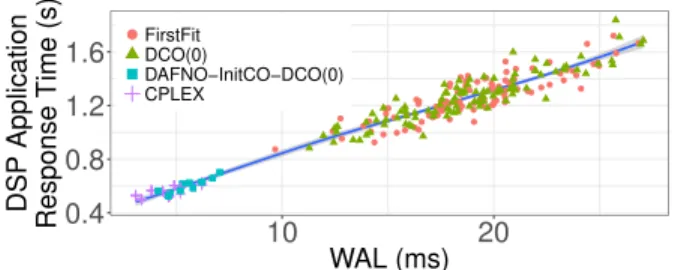
Three representative heuristic combinations—FirstFit (i.e., without any heuristic), DCO(0), and DAFNO-InitCO-DCO(0), are selected to compare with CPLEX. Figure 10shows obtained response times versus WAL values. ● ● ● ● ● ● ● ● ● ● ● ● ● ● ● ● ●● ● ● ● ● ● ● ● ● ● ● ● ● ● ● ● ● ● ● ● ● ● ● ● ● ● ● ● ● ● ● ●● ● ● ● ●● ● ● ● ●● ● ● ●●● ●● ● ●● ● ● ● ● ● ● ●● ● ● ● ● ● ● ● ● ● ● ● ● ● ● ● ● ● ● ● ●● ● 0.4 0.8 1.2 1.6 10 20 WAL (ms) DSP Application Response Time (s) ●_FirstFit DCO(0) DAFNO−InitCO−DCO(0) CPLEX

Figure 10: DSP Applications’ Response Time under Place-ments with Different WAL Values.

As illustrated in Figure 10, the response time in-creases with WAL. Their correlation is up to 0.976, which validates the objective function—minimizing WAL.

Taking the 10 placement problems into account, each evaluated algorithm’s average execution time and av-erage response time are summarized in Table VI. For each problem, obtained response times are normalized according to CPLEX’s, i.e., the response time under the optimal placement is regarded as 1 (100%).

Compared with FirstFit, DCO(0) has a much lowered execution time but a similar response time, which accelerates the search without improving the result

Algorithm Execution Response

Time (s) Time

FirstFit 756 230%

DCO(0) 0.011 229%

DAFNO-InitCO-DCO(0) 0.019 109%

CPLEX 258 100%

Table VI:Representative Heuristic Combinations vs CPLEX.

quality. DAFNO-InitCO-DCO(0) improves FirstFit on both execution time and response time. Compared with CPLEX, although DAFNO-InitCO-DCO(0) gets a 9% higher response time, it gains a 10000 times’ speed-up.

2) Impacts of DAFNO and InitCO: According to the previous evaluation in Section IV-C1, CPLEX arrives to place 1 application (with 16 components) in an infrastructure (with 27 fog nodes and 40 appliances) in 258 seconds. To compare different heuristic combina-tions’ scalability, given the same execution time—258 seconds, we evaluate how many applications / compo-nents each algorithm can place in a larger infrastructure containing: 1 cloud; 10 high edge servers (as edge server1 inFigure 8) randomly connected to each other, and each of them also connects with the cloud; 50 low edge servers (as edge server2∼3 inFigure 8), each con-nected with a random high edge server; 500 gateways, each connected with a random low edge server; 10000 end fog nodes and 20000 appliances, each connected with a random low edge server or gateway. Following resource capacity distributions given in Section IV-B, an infrastructure model is generated, which must cover different resource situations thanks to its large scale. Each algorithm places more and more applications until it exceeds the timeout of 258 seconds. Starting from 1 application, 25 randomly generated DSP applications are added each time.

According to the evaluation in the previous work [5], compared with FirstFit, AFNO, and DCO(1), AFNO-DCO(1) performs better on both scalability and result quality. This evaluation compares other heuristic com-binations with AFNO-DCO(1). The obtained execution times are depicted inFigure 11.

● ● ● ●● ● ● ● ● ● timeout 0 250 500 7501000 0 5 10 15 0 2500 5000 7500 0 100 200 300 400 500 Component Number Ex ecution Time (s)

Algorithms:●_{AFNO−DCO(1) DAFNO−DCO(1) DAFNO−InitCO−DCO(1)}

Figure 11: Execution Times with Growing Applications.

Due to the large infrastructure scale, FirstFit and CPLEX timeouts at the very beginning. Without DCO, algorithms DAFNO and DAFNO-InitCO only arrive to place 1 application within the timeout. According to Figure 11, once DCO is applied, the algorithm becomes much more scalable. As shown in the zoomed graph on the left of Figure 11, when there are not

many applications / components to place, DDCO(1) has a higher execution time than AFNO-DCO(1), which is caused by the overhead of updating anchors. However, with more applications concurrent to limited resources, anchors are easier to be outdated, and DAFNO-DCO(1) outperforms AFNO-DCO(1), which shows that up-to-date anchors help to accelerate the search. With random initial component orders, AFNO-DCO(1) and DAFNO-AFNO-DCO(1) introduce higher vari-ances than DAFNO-InitCO-DCO(1). It can also be found that DAFNO-InitCO-DCO(1) gets a better perfor-mance than DAFNO-DCO(1), especially when dealing with more than 5000 components. This is because of that, among considered constraints (see Section II-A), the constraint of bandwidth consumption is the most complicated, because: i) a link’s bandwidth can be consumed by multiple bindings; ii) a binding can pass by multiple links; iii) where a binding is placed can con-cern two components’ hosts; iv) one component can be connected by multiple bindings. Compared with other constraints’ violation (e.g., CPU), DCO can have to test many more component orders to avoid a failure caused by the bandwidth. Taking this complexity into account by satisfying priorly components with high bandwidth requirements (seeSection III-B), InitCO helps to reduce the number of components’ reorderings carried out by DCO and accelerate the search.

Response times obtained by evaluated algorithms are compared in Figure 12. For each application / compo-nent number, obtained response times are normalized according to InitCO-DCO(1)’s, i.e., DAFNO-InitCO-DCO(1)’s response time is regarded as 1.

● ● ● _● ● ● AFNO−DCO(1) timeout 100% 102% 104% 106% 2000 4000 6000 Component Number DSP Applications' _Aver age Response Time (nor maliz ed) ●_{AFNO−DCO(1)} DAFNO−DCO(1) DAFNO−InitCO−DCO(1)

Figure 12: Response Times with Growing Applications.

As shown inFigure 12, DAFNO-DCO(1)’s response time is always lower than AFNO-DCO(1), which vali-dates that dynamic anchors further lower applications’ response time compared with static ones. According to that DAFNO-InitCO-DCO(1) has a lower response time than DAFNO-DCO(1), and the difference increases with the component number, we conclude that InitCO also helps to reduce applications’ response time, especially when placing many applications / components.

According to execution times and response times obtained in this evaluation, based on AFNO-DCO(1), DAFNO and InitCO proposed in this work further enhance the algorithm’s scalability and result quality.

3) Impacts of Parameters stepLen and f ailN B:

According to the evaluation inSection IV-C2,

DAFNO-InitCO-DCO(1) (equivalent to

DAFNO-InitCO-DCO(1)-FailCap(∞)) arrives to place 426 applications (with 8589 components) in an infrastructure (with 10561 fog nodes and 20000 appliances) in about 270 seconds. This placement problem is reused to evaluate DAFNO-InitCO-DCO(stepLen)-FailCap(f ailN B) with different parameter settings. The evaluation results are depicted inFigure 13.

● ● ● ● ● ● 150 200 250 300 350 0.0 0.3 0.6 0.9 stepLen of DCO Ex ecution Time (s) (a) ● ● ● ● ● ● 99.3% 99.6% 99.9% 100.2% 0.0 0.3 0.6 0.9 stepLen of DCO DSP Applications' _Aver age Response Time (nor maliz ed) (b)

failNB of FailCap:●_{10 100 300 infinite}

Figure 13:Evaluation Results with Different Parameters.

As stated in Section III-B, a lower / higher stepLen leads to more / fewer component moves, but more / less reutilization of obtained search results. According to execution times shown in Figure 13 (a), stepLen values near to the two extremes (i.e., 0 and 1) can cause high execution times. Compared with DCO(1), a proper stepLen can further accelerate the search. On the other hand, compared with ∞, a lower f ailN B helps to lower execution times only when stepLen is assigned to a low value (e.g., as in Figure 13 (a) when stepLen = 0.1). The reduction of execution time becomes weak when stepLen ≥ 0.3. Moreover, a low f ailN B can miss proper fog nodes, cause more component reorderings, and get even higher execution times (e.g., as in Figure 13(a) when stepLen= 1).

A lower stepLen better respects the initial com-ponent order produced by InitCO. According to re-sponse times (normalized according to DAFNO-InitCO-DCO(1)’s) shown in Figure 13 (b), lower stepLen values help to get lower response times. However, a low f ailN B risks of missing proper fog nodes and resulting in a higher response time.

This evaluation shows that a low stepLen value of DCO helps to further improve the heuristic combina-tion’s result quality. However, a stepLen close to 0 causes high execution times when dealing with large-scale problems. Hence, a trade-off is needed to consider these two aspects. On the other hand, when stepLen is assigned to a proper value that helps to avoid high execution times, a f ailN B value lower than ∞ no longer reduces or even raises execution times.

To sum up, DAFNO-InitCO-DCO(stepLen) appears as the best compromise in terms of scalability and result quality (based on our experience with the evaluated use case, a stepLen value of 0.2∼0.4 is recommended). It gets solutions close to optimal ones obtained by CPLEX with much lowered execution times. It also enhances AFNO-DCO(1) proposed in [5] on both scalability and result quality. The proposed algorithm is highly scalable, through which we get a satisfactory placement of 8589 components in an infrastructure with 10561 fog

nodes within 200 seconds. Moreover, being able to deal with highly random problems (with randomly generated infrastructures / applications, see Section IV-B), the proposition is shown to be a generic approach.

V. RELATEDWORK

A number of works are related to this study. Among these works, [3]–[5], [9]–[12] focus on fog computing; [13], [14] are generic enough to suit both fog and cloud. From applications’ point of view, [4], [5], [9] deal with IoT applications. As fog computing is still a recently emerging research topic, other related works are rather in the context of cloud. Nevertheless, they are still worth to discuss. The related works are classified into exact algorithms, metaheuristics, and heuristics.

A. Exact Algorithms

[3], [12] formulate the placement problem with Inte-ger Linear Programming (ILP), and solve the problem using generic ILP-solvers, which guarantee to return the optimal solution.

An exhaustive algorithm [4], [5], which searches in a manner similar to FirstFit, ends the search until the search space is traversed (instead of finding the first solution), so that all solutions are visited, and the optimal one can be found out.

Exact algorithms always deliver the optimal solution. However, suffering from high execution time, they are hardly scalable.

B. Metaheuristics

Given a placement problem, metaheuristics visit only a part of the search space, and return the best placement among visited ones. Each metaheuristic has a specific strategy to get close to the optimum as fast as possible. Hill climbing [11], [15] improves a solution itera-tively. At each iteration, a randomly selected component is re-placed to better fit the objective function. However, starting from a random initial solution, it usually traps into a local optimum. To escape from local optimums, simulated annealing [16], [17] and tabu search [16], [18] allow visiting solutions with lower quality. However, these approaches can require a large number of itera-tions, which lower their scalability.

Genetic algorithm [10], [19], particle swarm opti-mization [20], [21], and ant colony optimization [22], [23] refine a predefined number of placements (i.e., a population) iteratively. At each iteration, new place-ments are generated and evaluated (regarding the opti-mization objective). These algorithms’ inner parameters, based on which placements are generated, are tuned dynamically according to the evaluation of generated placements. The best placement among tested ones is returned when a predefined timeout is reached. Conse-quently, the result quality is strongly related to prede-fined parameters (e.g., timeout, population size), whose proper values are use case-dependent and difficult to predict without experiment. Furthermore, given a place-ment problem, these approaches do not guarantee to find a solution, even if solutions exist.

By making use of the knowledge of applications’ appliance and DZs, our approach calculates anchors and guides the search to a satisfactory solution. Without such a guide but using random initial placement(s), metaheuristics can need more tests / a higher execution time to get a similar result quality.

C. Heuristics

Specialized heuristics are also designed to handle the placement problem. [14], [24] propose Best-Fit / Worst-Fit heuristic to consolidate / balance host loads. [25] chooses candidate hosts with higher renting cost-efficiency priorly to minimize the financial cost. How-ever, applications’ response time is not considered in these heuristics.

[13], [26] propose application response time-targeted heuristics. These approaches locate devices and compo-nents using geographic coordinates / a latency space (in which the distance between two devices represents the network latency between them). Components’ coordi-nates are initialized according to coordicoordi-nates of devices tied to considered applications. Then, each component’s coordinate is refined by an iterative algorithm to better fit the optimization objective. Finally, each component is placed in its nearest device that has enough resources to host it. Instead of using continuous coordinates, our approach directly use fog nodes as components’ anchors, which helps to reduce the algorithm’s number of iteration and avoids mapping coordinates to devices (the nearest device to the optimal coordinate is not guaranteed to be the optimal). Moreover, our approach updates anchors dynamically to keep them up-to-date, which is not considered in these works.

To deal with large-scale problems, [27] priorly places a component that requires more CPU / RAM / DISK resources; [9] places first a component that has less fog nodes in its DZ. They consider components’ con-currence to CPU / RAM / DISK resources in a static manner. However, during a search, available resources in the infrastructure evolve each time when a component is placed. Without considering such resource evolution and the limit of network resources, these approaches are still quite probable to encounter backtracks leading to huge amounts of tests. By making use of the knowledge obtained during the search and adjusting components’ order dynamically, our approach avoids backtracks and can be much more scalable and generic.

VI. CONCLUSION ANDFUTUREWORK

This paper tackles the problem of placing IoT appli-cations in the fog, that is how to map a set of software components onto a set of fog nodes. The focus of this work is on placement approaches’ scalability and result quality. The scalability is assessed through problem size (i.e., components’ number and fog nodes’ number) that an algorithm can deal with under a timeout, and the placement quality is expressed as average response time of placed applications.

Contributions of this paper are: i) four heuristics (DAFNO, InitCO, DCO, and FailCap) that can be com-bined with each other; ii) a simulation-based evaluation that compares different heuristic combinations.

The evaluation shows that: i) each proposed heuristic can accelerate the algorithm and / or lower applica-tions’ response times; ii) compared with the heuristic combination AFNO-DCO(1) proposed in [5], DAFNO-InitCO-DCO(stepLen), which combines heuristics pro-posed in this work, performs better on both scalability and result quality.

Our future works include: i) enhancements of the proposed placement approach to handle the intrinsic volatility of fog infrastructures (e.g., devices’ churn and mobility); ii) re-optimization of the placement taking applications’ arrival, departure, and the migration cost of deployed applications into account; iii) evaluation with experiment on industrial testbeds (such as the Orange Labs internal testbed introduced in [28]).

REFERENCES

[1] Flavio Bonomi, Rodolfo Milito, Jiang Zhu, and Sateesh Adde-palli. Fog computing and its role in the internet of things. In

Proceedings of the first edition of the MCC workshop on Mobile

cloud computing, pages 13–16. ACM, 2012.

[2] Luis M Vaquero and Luis Rodero-Merino. Finding your way in the fog: Towards a comprehensive definition of fog computing.

ACM SIGCOMM Computer Communication Review, 44(5):27–

32, 2014.

[3] Valeria Cardellini, Vincenzo Grassi, Francesco Lo Presti, and Matteo Nardelli. Optimal operator placement for distributed stream processing applications. In Proceedings of the 10th

ACM International Conference on Distributed and Event-based

Systems, pages 69–80. ACM, 2016.

[4] Antonio Brogi, Stefano Forti, and Ahmad Ibrahim. How to best deploy your fog applications, probably. In International

Conference on Edge and Fog Computing, 2017.

[5] Ye Xia, Xavier Etchevers, Lo¨ıc Letondeur, Thierry Coupaye, and Fr´ed´eric Desprez. Combining Hardware Nodes and Soft-ware Components Ordering-based Heuristics for Optimizing the Placement of Distributed IoT Applications in the Fog. In The

33rd ACM/SIGAPP Symposium On Applied Computing. ACM,

2018, (in press).

[6] Marcos Dias de Assuncao, Alexandre da Silva Veith, and Rajkumar Buyya. Resource elasticity for distributed data stream processing: A survey and future directions. arXiv preprint

arXiv:1709.01363, 2017.

[7] Henri Casanova, Arnaud Giersch, Arnaud Legrand, Martin Quinson, and Fr´ed´eric Suter. Versatile, scalable, and accurate simulation of distributed applications and platforms. Journal of

Parallel and Distributed Computing, 74(10):2899–2917, 2014.

[8] Cplex toolkit. http://www.ibm.com/support/knowledgecenter/ SSSA5P. Accessed: 2018-02-08.

[9] Antonio Brogi and Stefano Forti. Qos-aware deployment of iot applications through the fog. IEEE Internet of Things Journal, 2017.

[10] Olena Skarlat, Matteo Nardelli, Stefan Schulte, Michael Borkowski, and Philipp Leitner. Optimized IoT service place-ment in the fog. Service Oriented Computing and Applications, pages 1–17, 2017.

[11] William T¨arneberg, Amardeep Mehta, Eddie Wadbro, Johan Tordsson, Johan Eker, Maria Kihl, and Erik Elmroth. Dynamic application placement in the mobile cloud network. Future

Generation Computer Systems, 70:163–177, 2017.

[12] Olena Skarlat, Matteo Nardelli, Stefan Schulte, and Schahram Dustdar. Towards qos-aware fog service placement. In Fog

and Edge Computing (ICFEC), 2017 IEEE 1st International

Conference on, pages 89–96. IEEE, 2017.

[13] Stamatia Rizou, Frank D¨urr, and Kurt Rothermel. Solving the multi-operator placement problem in large-scale operator networks. In ICCCN, pages 1–6, 2010.

[14] Mina Sedaghat, Francisco Hern´andez-Rodriguez, and Erik Elm-roth. Autonomic resource allocation for cloud data centers: A peer to peer approach. In Cloud and Autonomic Computing

(ICCAC), 2014 International Conference on, pages 131–140.

IEEE, 2014.

[15] Emiliano Casalicchio, Daniel A Menasc´e, and Arwa Aldhalaan. Autonomic resource provisioning in cloud systems with avail-ability goals. In Proceedings of the 2013 ACM Cloud and

Autonomic Computing Conference, page 1. ACM, 2013.

[16] Ioannis A Moschakis and Helen D Karatza. A meta-heuristic optimization approach to the scheduling of bag-of-tasks appli-cations on heterogeneous clouds with multi-level arrivals and critical jobs. Simulation Modelling Practice and Theory, 57:1– 25, 2015.

[17] Yongqiang Wu, Maolin Tang, and Warren Fraser. A simulated annealing algorithm for energy efficient virtual machine place-ment. In Systems, Man, and Cybernetics (SMC), 2012 IEEE

International Conference on, pages 1245–1250. IEEE, 2012.

[18] Fatos Xhafa, Javier Carretero, Bernab´e Dorronsoro, and Enrique Alba. A tabu search algorithm for scheduling independent jobs in computational grids. Computing and informatics, 28(2):237– 250, 2012.

[19] Maolin Tang and Shenchen Pan. A hybrid genetic algorithm for the energy-efficient virtual machine placement problem in data centers. Neural Processing Letters, 41(2):211–221, 2015. [20] An-ping Xiong and Chun-xiang Xu. Energy efficient

multire-source allocation of virtual machine based on pso in cloud data center. Mathematical Problems in Engineering, 2014, 2014. [21] Elina Pacini, Cristian Mateos, and Carlos Garc´ıa Garino.

Dy-namic scheduling based on particle swarm optimization for cloud-based scientific experiments. CLEI Electronic Journal, 17(1):3–3, 2014.

[22] Md Hasanul Ferdaus, Manzur Murshed, Rodrigo N Calheiros, and Rajkumar Buyya. Virtual machine consolidation in cloud data centers using aco metaheuristic. In European Conference

on Parallel Processing, pages 306–317. Springer, 2014.

[23] Yongqiang Gao, Haibing Guan, Zhengwei Qi, Yang Hou, and Liang Liu. A multi-objective ant colony system algorithm for virtual machine placement in cloud computing. Journal of

Computer and System Sciences, 79(8):1230–1242, 2013.

[24] Wubin Li, Johan Tordsson, and Erik Elmroth. Virtual machine placement for predictable and time-constrained peak loads. In International Workshop on Grid Economics and Business

Models, pages 120–134. Springer, 2011.

[25] Pedro Silva, Christian Perez, and Fr´ed´eric Desprez. Efficient heuristics for placing large-scale distributed applications on mul-tiple clouds. In Cluster, Cloud and Grid Computing (CCGrid),

2016 16th IEEE/ACM International Symposium on, pages 483–

492. IEEE, 2016.

[26] Sharad Agarwal, John Dunagan, Navendu Jain, Stefan Saroiu,

Alec Wolman, and Harbinder Bhogan. Volley: Automated

data placement for geo-distributed cloud services. In NSDI, volume 10, pages 28–0, 2010.

[27] Xunyun Liu and Rajkumar Buyya. Performance-oriented de-ployment of streaming applications on cloud. IEEE Transactions

on Big Data, 2017.

[28] Letondeur Lo¨ıc, Ottogalli Franois-Ga¨el, and Coupaye Thierry. A demo of application lifecycle management for IoT collaborative neighborhood in the fog - Practical experiments and lessons learned around docker. In Fog World Congress. IEEE, 2017.