CAMS-72 Solar radiation products, Regular Validation Report, J-J-A 2017

(1)

HAL Id: hal-01969518

https://hal-mines-paristech.archives-ouvertes.fr/hal-01969518

Submitted on 4 Jan 2019

HAL is a multi-disciplinary open access

archive for the deposit and dissemination of sci-entific research documents, whether they are pub-lished or not. The documents may come from teaching and research institutions in France or abroad, or from public or private research centers.

L’archive ouverte pluridisciplinaire HAL, est destinée au dépôt et à la diffusion de documents scientifiques de niveau recherche, publiés ou non, émanant des établissements d’enseignement et de recherche français ou étrangers, des laboratoires publics ou privés.

CAMS-72 Solar radiation products, Regular Validation

Report, J-J-A 2017

Mireille Lefèvre, Lucien Wald

To cite this version:

Mireille Lefèvre, Lucien Wald. CAMS-72 Solar radiation products, Regular Validation Report, J-J-A 2017. [Technical Report] 19, Copernicus Atmosphere Monitoring Service. 2018. �hal-01969518�

(2)

ECMWF COPERNICUS REPORT

Copernicus Atmosphere Monitoring Service

D72.2.3.1

Regular Validation Report

Issue #19

J-J-A 2017

CAMS-72

Solar radiation products

Issued by: Armines / M. Lefèvre, L. Wald

Date: 26/03/2018

(3)

This document has been produced in the context of the Copernicus Atmosphere Monitoring Service (CAMS).

The activities leading to these results have been contracted by the European Centre for Medium-Range Weather Forecasts, operator of CAMS on behalf of the European Union (Delegation Agreement signed on 11/11/2014). All information in this document is provided "as is" and no guarantee or warranty is given that the information is fit for any particular purpose. The user thereof uses the information at its sole risk and liability. For the avoidance of all doubts, the European Commission and the European Centre for Medium-Range Weather Forecasts has no liability in respect of this document, which is merely representing the authors view.

(4)

Copernicus Atmosphere Monitoring Service

Contributors

ARMINES

Mireille Lefèvre

Lucien Wald

(5)

1. Introduction

7

2. Sources of data and stations

9 2.1 Typical uncertainty of measurements

9 2.2 Definitions of the measured radiation variables

10 2.3 Sources of data

11 2.4 Short description of the stations selected for the validation and maps

12 2.5 List of the stations retained for this quarter

15

3. Overview of the results

17 3.1 Global irradiance

17 3.2 Diffuse irradiance

19 3.3 Direct irradiance at normal incidence

20

4. Discussion

22 4.1 Global irradiance

Error! Bookmark not defined.

4.2 Ability to reproduce the intra-day variability

22 4.3 Bias and standard deviation of errors

22 4.4 Ability to reproduce the frequency distributions of measurements

24 4.5 Ability to reproduce the monthly means and standard deviation for the period

26 4.6 Summary

27

5. Acknowledgements

28

6. Reference documents

29 Annex A. Procedure for validation

31 1. Taking care of the time system

31 2. Taking care of missing data within an hour or one day

32 3. Computation of deviations and statistical quantities

32 4. Comparison of histograms and monthly means

34 Annex. Station TORAVERE

35 Annex. Station ZOSENI

43 Annex. Station RIGA

49

(6)

Annex. Station LIEPAJA

61 Annex. Station RUCAVA

67 Annex. Station HOORN

73 Annex. Station HOOGEVEEN

79 Annex. Station TWENTHE

85 Annex. Station CABAUW

91 Annex. Station VLISSINGEN

97 Annex. Station POPRAD-GANOVCE

103 Annex. Station BANSKA-BYSTRICA

111 Annex. Station KISHINEV

116 Annex. Station CARPENTRAS

123 Annex. Station TAMANRASSET

130 Annex. Station GOBABEB

137

(7)

(8)

1. Introduction

Outcomes of the CAMS Radiation Service have to be validated on a periodic basis. Following

practices in CAMS, this validation is performed every trimester. Following current practices

in assessment of satellite-derived data in solar energy, the irradiances provided by the CAMS

Radiation Service are tested against qualified ground measurements measured in several

ground-based stations serving as reference. These ground measurements are coincident in

time with the CAMS Radiation Service estimates.

This report is the issue #19 of a regular report. It deals with hourly means of global, diffuse,

and direct irradiances for the period June-July-August 2017, abbreviated as JJA 2017.

On 2017-10-11, version 3 of the CAMS Radiation Service was introduced. By construction,

the CAMS Radiation Service performs the calculation of the radiation on-the-fly at the

request of any user. It processes on-the-fly the necessary information that is stored in CAMS

and does not create a proper database of the results. Hence, the new version 3 applies from

now on back to 2004-02-01.

The main change in v3 for users is the reduction of the bias. Other changes in the new

version are small for most users. Potential discontinuities in time series, within a day or

throughout the year, or maps have been removed by revising the process. Major changes

are found in the process itself, permitting the removal of these discontinuities and easing

future changes in the process.

This validation report is performed with version 3 of the CAMS Radiation Service. The

previous issues up to #17 were performed with version 2. The changes between v2 and v3

have been documented and reports are available on the CAMS website. Nevertheless, for

helping users better, two validation reports are available, one using v2 and the other using

v3, for the same stations and a winter period (DJF 2017) and a summer period (JJA 2017).

The issue #17 provided in September 2017 deals with v2 for DJF 2017; the issue #17b

delivered in December 2017 deals with v3 for the same sites and same period. The current

issue #19 deals with v3 and JJA 2017, while the issue #19b deals with v2 for the same sites

and same period. By comparing the two versions of the two issues #17 and #19, users can

have a deep insight of the changes.

The results discussed in this report may be retrieved for several of the selected stations and

others by running the service “Irradiation Validation Report” at the SoDa Web site:

(9)

This service “Irradiation Validation Report” performs a comparison of the hourly or daily

solar irradiation at surface estimated by the CAMS Radiation Service against several qualified

ground measurements obtained from various sources. It returns a HTML page that contains

statistics of comparisons and graphs. Similar calculations can be done for the estimates from

HelioClim-3 version 4 and HelioClim-3 version 5. The time coverage of the CAMS Radiation

Service and HelioClim-3 version 5 databases is from 2004-02-01 up to 2 days ago, and up to

d-1 for the HelioClim-3 version 4. Each station has its own temporal coverage of

measurements, and the period of comparison must be selected within this period of data

availability. The geographical coverage is the field-of-view of the Meteosat satellite, roughly

speaking Europe, Africa, Atlantic Ocean, and Middle East (-66° to 66° in both latitudes and

longitudes).

(10)

2. Sources of data and stations

Measurements are taken from various sources and measuring stations that are discussed in

this section.

2.1 Typical uncertainty of measurements

The World Meteorological Organization (WMO, 2012) sets recommendations for achieving a

given accuracy in measuring solar radiation. This document clearly states that “good quality

measurements are difficult to achieve in practice, and for routine operations, they can be

achieved only with modern equipment and redundant measurements.” The following Tables

report the typical uncertainty (95% probability) that can be read in the WMO document.

Additions were brought to the original table as uncertainties are now expressed in J m

-

_{² and}

W m

-

_².

Table 2.1. Typical uncertainty (95% probability) of measurements made by pyranometers (source: WMO 2012)

Good quality

Moderate quality

Hourly irradiation

8%

if irradiation is greater than

0.8 MJ m

-

_{². Otherwise}

uncertainty is 0.06 MJ m

-

_{², i.e.}

6 J cm

-

_{², or for irradiance}

approx. 20 W m

-

_²

20%

if irradiation is greater than

0.8 MJ m

-

_{². Otherwise}

uncertainty is 0.16 MJ m

-

_{², i.e.}

16 J cm

-

_{², or for irradiance}

approx. 50 W m

-

_²

Daily irradiation

5%

if irradiation is greater than

8 MJ m

-

_{². Otherwise,}

uncertainty is set to

0.4 MJ m

-

_{², i.e. 40 J cm}

-

_{², or for}

irradiance approx. 5 W m

-

_²

10%

if irradiation is greater than

8 MJ m

-

_{². Otherwise,}

uncertainty is set to

0.8 MJ m

-

_{², i.e. 80 J cm}

-

_{², or for}

irradiance approx. 9 W m

-

_²

(11)

Table 2.2. Typical uncertainty (95% probability) of measurements made by pyrheliometers (source: WMO 2012)

High quality

Good quality

1 min irradiation

0.9%

0.56 kJ m

-2

approx. 9 W m

-2

1.8%

1 kJ m

-2

approx. 17 W m

-2

Hourly irradiation

0.7%

21 kJ m

-2

approx. 6 W m

-2

1.5%

54 kJ m

-2

approx. 15 W m

-2

Daily irradiation

0.5%

200 kJ m

-2

approx. 2 W m

-2

1.0%

400 kJ m

-2

approx. 5 W m

-2

2.2 Definitions of the measured radiation variables

The hourly global irradiation G

energy

h is the amount of energy received during one hour on a

horizontal plane at ground level. It is also known as hourly global horizontal irradiation, or

hourly surface solar irradiation. Similarly, the hourly diffuse irradiation D

energy

h is the amount

of energy received from all directions of the sky vault, except that of the sun during one hour

on a horizontal plane at ground level, and the hourly direct (or beam) irradiation B

energy

h is

the amount of energy received from the direction of the sun during one hour on this

horizontal plane.

The hourly global irradiation G

energy

h is the sum of B

energy

h and D

energy

h. The hourly mean of

global irradiance Gh, respectively direct irradiance B

horizontal

h and diffuse irradiance Dh, is

equal to G

energy

h, respectively B

energy

h and D

energy

h, divided by 3600 s.

The hourly mean of direct irradiance at normal incidence Bh is the irradiance received from

the direction of the sun during one hour on a plane always normal to the direction of the

sun. See Blanc et al. (2014) for more details on the definition of the direct irradiance at

normal incidence and the incidence of the circumsolar radiation.

For the sake of simplicity, the notation h is abandoned in this text from now on. The hourly

means of global and diffuse irradiances are noted G and D, and the hourly mean of the direct

irradiance at normal incidence is noted B.

The hourly clearness index KT is defined as the ratio of G to the hourly extra-terrestrial

irradiance G0: KT = G / G0. The extra-terrestrial irradiance is computed here by the means of

the SG2 algorithm (Blanc, Wald, 2012). The direct clearness index and the diffuse clearness

index are defined in a similar way. Because the ratio of the direct horizontal to the direct

normal is equal to the cosine of the solar zenithal angle at both ground level and top of

(12)

atmosphere, it comes that the direct clearness index is the same than the direct normal

clearness index.

2.3 Sources of data

Efforts are made to build the quarterly validation reports with the same set of stations to

better follow and monitor the quality of the irradiance products delivered by the CRS though

this is difficult as discussed later.

Measurements originate from different networks as reported in Table 2.3. They have been

acquired in different time systems (UT: Universal Time, TST: True Solar Time). No change in

time system is performed during this validation. The handling of the different time systems is

described in the annex describing the procedure for validation.

Table 2.3. Source of data for each station, time system (UT: universal time; TST: true solar time) and type of data (G, B, D stands respectively for global, direct at normal incidence and diffuse). Ordered

from North to South.

Station Source of data Time

system Initial summarization Type of data acquired

Toravere BSRN UT 1 min G B D

Zoseni Latvian Environment, Geology and Meteorology Centre (LEGMC)

TST 1 h G

Riga Latvian Environment, Geology and Meteorology Centre (LEGMC)

TST 1 h G

Dobele Latvian Environment, Geology and Meteorology Centre (LEGMC)

TST 1 h G B -

Liepaja Latvian Environment, Geology and Meteorology Centre (LEGMC)

TST 1 h G

Rucava Latvian Environment, Geology and Meteorology Centre (LEGMC)

TST 1 h G

Daugavpils Latvian Environment, Geology and Meteorology Centre (LEGMC)

TST 1 h G

Silutes Lithuanian Hydrometeorological

Service (LHMS) UT 1 h G B -

Kauno Lithuanian Hydrometeorological

Service (LHMS) UT 1 h G B -

Hoorn KNMI UT 1 h G

(13)

Twenthe KNMI UT 1 h G

Cabauw KNMI UT 1 h G

Vlissingen KNMI UT 1 h G

Camborne BSRN UT 1 min G B D

Poprad-Ganovce Slovak Hydrometeorological

Institute (SHMI) UT 1 min G B D

Banska-Bystrica Slovak Hydrometeorological

Institute (SHMI) UT 1 min G - D

Milhostov Slovak Hydrometeorological

Institute (SHMI) UT 1 min G - D

Kishinev ARG / Academy of Sciences of

Moldova UT 1 min G B D

Carpentras BSRN UT 1 min G B D

Tatouine EnerMENA UT 1 min G B D

Missour EnerMENA UT 1 min G B D

Ma’an EnerMENA UT 1 min G B D

Tamanrasset BSRN UT 1 min G B D

Gobabeb BSRN UT 1 min G B D

Florianopolis BSRN UT 1 min G B D

2.4 Short description of the stations selected for the validation and maps

The selected stations are located in Europe, Africa and South America. Their geographical

coordinates are given in Table 2.4.

Table 2.4. List of stations used to realize the validation report in general, and their coordinates Country Station Latitude Longitude Elevation a.s.l. (m)

Estonia Toravere 58.254 26.462 70 Latvia Zoseni 57.135 25.906 188 Latvia Riga 56.951 24.116 6 Latvia Dobele 56.620 23.320 42 Latvia Liepaja 56.475 21.021 4 Latvia Rucava 56.162 21.173 19 Latvia Daugavpils 55.870 26.617 98 Lithuania Silutes 55.352 21.447 5 Lithuania Kauno 54.884 23.836 77

The Netherlands Hoorn 53.393 5.346 0

The Netherlands Hoogeveen 52.750 6.575 16

The Netherlands Twenthe 52.273 6.897 34

The Netherlands Cabauw 51.972 4.927 -1

The Netherlands Vlissingen 51.442 3.596 8

United Kingdom Camborne 50.217 -5.317 88

(14)

Copernicus Atmosphere Monitoring Service Slovakia Banska-Bystrica 48.734 19.117 427 Moldova Kishinev 47.000 28.817 205 France Carpentras 44.083 5.059 100 Tunisia Tataouine 32.974 10.485 210 Morocco Missour 32.860 -4.107 1107 Jordan Ma'an 30.172 35.818 1012 Algeria Tamanrasset 22.790 5.529 1385 Namibia Gobabeb -23.561 15.042 407 Brasilia Florianopolis -27.605 -48.523 11

Figure 2.1 (Europe) and Figure 2.2 (other regions) show the location of the stations with

their name and elevation above mean sea level. Symbols code the initial summarization of

the data as reported in Table 2.3: circle for 1 min, and downward triangle for 1 h. Colors

code the type of data at each site: red for (G, B, D), yellow for (G, B), magenta for (G, D) and

cyan for G.

Figure 2.1. Map showing the stations in Europe. Symbols code the initial summarization: circle for 1 min, and downward triangle for 1 h. Colors code the type of data at each site: red for (G, B, D),

(15)

Figure 2.2. Map showing part of the stations. Symbols code the initial summarization: circle for 1 min, and downward triangle for 1 h. Colors code the type of data at each site: red for (G, B, D), yellow for (G, B), magenta for (G, D) and cyan for G.

The selected stations are located in several different climates as reported in Table 2.5. The

description of climates is taken from the updated world map of the Köppen-Geiger climate

classification by Peel et al. (2007).

(16)

Table 2.5. List of climates and corresponding stations

Climate Stations

Dfa: Cold climate without dry season and hot

summer Poprad-Ganovce, Banska-Bystrica, Milhostov Dfb: Cold climate without dry season and warm

summer Toravere, Zoseni, Riga, Dobele, Liepaja, Rucava, Silutes, Kauno, Kishinev Cfa: Temperate climate without dry season and

hot summer Florianopolis

Cfb: Temperate climate without dry season and

warm summer Hoorn, Hoogeveen, Twenthe, Cabauw, Vlissingen, Camborne Csa: Temperate climate with dry and hot summer Missour

Csb: Temperate climate with dry and warm

summer Carpentras

BWh: Arid and hot climate of desert type Tataouine, Ma'an, Tamanrasset BWk: Arid and cold climate of desert type Gobabeb

BSh: Arid and hot climate of steppe type -

Among the set of stations, are several stations, such as Toravere, which are at the edge of

the field of view of the Meteosat Second Generation satellites and most likely at the edge of

physical assumptions used when retrieving cloud properties. This validation is meant to

include extreme cases into the station list.

One may note that though the validation aims at validating the variables G, B, and D

delivered by the CRS, several stations are included that measure only the global irradiance G.

They have been selected in order to check the spatial consistency of the quality of the CRS

products within in the same network and same climate. Figure 2.1 shows several groups of

stations that are close to each other within the same climate: the Eastern Baltic area, The

Netherlands, and Slovakia. One expects similar performances of CRS within a group.

2.5 List of the stations retained for this quarter

Depending on the provision of fresh data, possible problems affecting measuring

instruments, possible rejection of some data by the quality control, and other causes, it is

not always possible to use the same set of stations to perform the quarterly validation. Table

2.6 lists the stations that have retained for this quarter.

(17)

Table 2.6. List of stations retained for this regular validation report

Station Variables Station Variables

Toravere G B D Cabauw G Zoseni G Vlissingen G Riga G Poprad-Ganovce G B D Dobele G B - Banska-Bystrica G - D Liepaja G Kishinev G B D Rucava G Carpentras G B D Daugavpils G Tamanrasset G B D Hoorn G Gobabeb G B D Hoogeveen G Florianopolis G B D Twenthe G

(18)

3. Overview of the results

Following the ISO standard (1995), the deviations are computed by subtracting observations

for each instant from the product estimations (CRS - measurements), and are summarized by

usual statistical quantities such as the bias or the root mean square error. The validation

procedure is described in Annex A. Detailed results are given for each station in Annexes.

3.1 Global irradiance

The following tables summarize the performances of CRS for hourly mean of global

irradiance (in W m

-2

_{, Table 3.1) and corresponding clearness index (Table 3.2), and the}

performances relative to the mean of measurements (in percent, Table 3.3).

Table 3.1. Summary of the performances for hourly mean of global irradiance (in W m-_²)

Station Mean of

measurements Bias RMSE deviation Standard Correlation coefficient

Toravere 329 21 94 91 0.913 Zoseni 327 28 97 92 0.907 Riga 345 3 103 103 0.894 Dobele 350 -9 90 90 0.911 Liepaja 373 -20 90 88 0.936 Rucava 360 3 86 86 0.935 Daugavpils 342 18 98 96 0.913 Hoorn 365 -44 91 80 0.952 Hoogeveen 343 22 84 81 0.936 Twenthe 327 28 85 80 0.935 Cabauw 359 23 85 82 0.936 Vlissingen 384 -21 81 79 0.953 Poprad-Ganovce 422 20 104 102 0.926 Banska-Bystrica 429 17 95 94 0.936 Kishinev 467 -7 69 69 0.968 Carpentras 500 -1 52 52 0.984 Tamanrasset 547 -16 98 97 0.961 Gobabeb 469 -20 26 17 0.998 Florianopolis 339 -7 57 56 0.964

Table 3.2. Summary of the performances for hourly global clearness index

Station Mean of

Toravere 0.468 0.019 0.124 0.123 0.797

Zoseni 0.444 0.035 0.131 0.126 0.781

Riga 0.484 -0.015 0.186 0.185 0.601

Dobele 0.529 -0.043 0.219 0.215 0.463

(19)

Copernicus Atmosphere Monitoring Service Rucava 0.506 -0.012 0.152 0.152 0.757 Daugavpils 0.459 0.020 0.140 0.139 0.781 Hoorn 0.473 -0.061 0.115 0.098 0.884 Hoogeveen 0.446 0.022 0.102 0.100 0.864 Twenthe 0.424 0.031 0.101 0.096 0.872 Cabauw 0.460 0.025 0.104 0.101 0.863 Vlissingen 0.485 -0.026 0.102 0.098 0.876 Poprad-Ganovce 0.538 0.015 0.122 0.121 0.809 Banska-Bystrica 0.532 0.019 0.115 0.113 0.817 Kishinev 0.566 -0.009 0.094 0.094 0.866 Carpentras 0.601 0.000 0.072 0.072 0.900 Tamanrasset 0.576 -0.010 0.106 0.105 0.865 Gobabeb 0.692 -0.035 0.053 0.040 0.942 Florianopolis 0.518 -0.009 0.086 0.085 0.910

Table 3.3. Summary of the performances for hourly mean of global irradiance and corresponding clearness index relative to the mean of measurements (in percent)

Station Rel. bias Rel. RMSE Rel. stand.

dev. Rel. bias Rel. RMSE Rel. stand. dev.

Toravere 6 28 27 4 26 26 Zoseni 8 29 28 7 29 28 Riga 0 29 29 -3 38 38 Dobele -2 25 25 -8 41 40 Liepaja -5 24 23 -7 26 25 Rucava 0 23 23 -2 30 29 Daugavpils 5 28 28 4 30 30 Hoorn -11 24 21 -12 24 20 Hoogeveen 6 24 23 5 22 22 Twenthe 8 25 24 7 23 22 Cabauw 6 23 22 5 22 21 Vlissingen -5 21 20 -5 20 20 Poprad-Ganovce 4 24 24 2 22 22 Banska-Bystrica 3 22 21 3 21 21 Kishinev -1 14 14 -1 16 16 Carpentras 0 10 10 0 12 12 Tamanrasset -2 17 17 -1 18 18 Gobabeb -4 5 3 -5 7 5 Florianopolis -2 16 16 -1 16 16

(20)

3.2 Diffuse irradiance

The following tables summarize the performances of CRS for hourly mean of diffuse

irradiance (in W m

-2

_{, Table 3.4) and corresponding clearness index (Table 3.5), and the}

performances relative to the mean of measurements (in percent, Table 3.6).

Table 3.4. Summary of the performances for hourly mean of diffuse irradiance (in W m-_²)

Station Mean of

Toravere 161 9 60 59 0.795 Poprad-Ganovce 166 2 52 52 0.867 Banska-Bystrica 159 4 50 50 0.862 Kishinev 146 0 43 43 0.886 Carpentras 137 4 43 42 0.888 Tamanrasset 252 -58 106 89 0.855 Gobabeb 84 22 33 24 0.817 Florianopolis 132 -6 46 46 0.849

Table 3.5. Summary of the performances for hourly diffuse clearness index

Station Mean of

Toravere 0.233 0.011 0.081 0.080 0.543 Poprad-Ganovce 0.219 0.003 0.062 0.062 0.733 Banska-Bystrica 0.210 0.004 0.060 0.059 0.732 Kishinev 0.186 0.002 0.052 0.052 0.784 Carpentras 0.180 0.004 0.050 0.050 0.852 Tamanrasset 0.287 -0.061 0.106 0.087 0.603 Gobabeb 0.137 0.035 0.050 0.035 0.820 Florianopolis 0.204 -0.005 0.064 0.064 0.761

Table 3.6. Summary of the performances for hourly mean of diffuse irradiance and corresponding clearness index relative to the mean of measurements (in percent)

Station Rel. bias Rel. RMSE Rel. stand.

Toravere 5 37 36 4 34 34 Poprad-Ganovce 1 31 31 1 28 28 Banska-Bystrica 2 31 31 2 28 28 Kishinev 0 29 29 0 27 27 Carpentras 3 31 31 2 28 27 Tamanrasset -23 42 35 -21 36 30 Gobabeb 26 39 29 25 36 25 Florianopolis -4 34 34 -2 31 31

(21)

3.3 Direct irradiance at normal incidence

The following tables summarize the performances of CRS for hourly mean of direct

irradiance at normal incidence (in W m

-2

_{, Table 3.7) and corresponding clearness index}

(Table 3.8), and the performances relative to the mean of measurements (in percent, Table

3.9).

Table 3.7. Summary of the performances for hourly mean of direct irradiance at normal incidence (in W m-_²)

Station Mean of

Toravere 419 -22 183 182 0.753 Dobele 386 -41 168 163 0.760 Poprad-Ganovce 478 0 158 158 0.840 Kishinev 549 -27 121 118 0.903 Carpentras 574 -20 105 104 0.934 Tamanrasset 419 82 178 158 0.828 Gobabeb 649 -82 108 71 0.971 Florianopolis 506 -13 135 135 0.886

Table 3.8. Summary of the performances for hourly direct clearness index

Station Mean of

Toravere 0.317 -0.017 0.139 0.138 0.753 Dobele 0.293 -0.032 0.128 0.124 0.753 Poprad-Ganovce 0.362 0.000 0.120 0.120 0.838 Kishinev 0.416 -0.021 0.092 0.090 0.901 Carpentras 0.435 -0.015 0.080 0.078 0.934 Tamanrasset 0.317 0.063 0.135 0.120 0.828 Gobabeb 0.502 -0.069 0.088 0.054 0.965 Florianopolis 0.384 -0.010 0.103 0.103 0.883

Table 3.9. Summary of the performances for hourly mean of direct irradiance at normal incidence and corresponding clearness index relative to the mean of measurements (in percent) Station Rel. bias Rel. RMSE Rel. stand.

Toravere -5 43 43 -5 43 43 Dobele -10 43 42 -10 43 42 Poprad-Ganovce 0 33 33 0 33 33 Kishinev -4 22 21 -5 22 21 Carpentras -3 18 18 -3 18 17 Tamanrasset 19 42 37 19 42 37

(22)

Gobabeb -12 16 10 -13 17 10

(23)

4. Discussion

4.1 Ability to reproduce the intra-day variability

The CRS estimates for global irradiance correlate very well with the measurements. All

correlation coefficients for this quarter are greater than 0.89 and very often greater than

0.95. The correlation coefficient for irradiance exhibits a clear tendency to increase with the

mean clearness index of the sites.

As expected, the correlation coefficients are smaller for the clearness index. Nevertheless,

they are greater than 0.76, except at Dobele (0.46) and Riga (0.60), and very often greater

than 0.85. The tendency of the correlation coefficient to increase as the clearness index

increases is less marked than for the irradiance.

One may note that the correlation coefficients are consistent within the same network or

same area. The sites from Estonia and Latvia offer similar coefficients. This is also the case

for the sites in The Netherlands or in Slovakia.

As for the diffuse irradiance and the diffuse clearness index, the correlation coefficients are

slightly less than for global. They range between 0.80 (Toravere) and 0.89 (Kishinev and

Carpentras) for irradiance and between 0.54 (Toravere) and 0.85 (Carpentras) for clearness

index. It can be concluded that the hour-to-hour variability of the diffuse radiation is

reproduced by CRS.

The correlation coefficients for both the direct irradiance and the direct clearness index are

similar –as expected because the diffuse is computed as the subtraction of the direct to the

global- and range from 0.75 (Toravere) to 0.97 (Gobabeb) for irradiance and from 0.75

(Toravere and Dobele) to 0.97 (Gobabeb) for the clearness index.

4.2 Bias and standard deviation of errors

The following empirical rules are adopted for the bias and the standard deviation (Table 4.1).

They are derived from the uncertainty (20 W m

-2

_{) of the measurements of hourly irradiation}

of good quality from the recommendations of the WMO (see Table 2.1).

Table 4.1. Rules for the bias and the standard deviation (in W m-_²)

Null bias Absolute value of the bias ≤ 5 Low bias 5 < absolute value of the bias ≤ 10 Noticeable bias 10 < absolute value of the bias ≤ 20 Large bias 20 < absolute value of the bias ≤ 60 Very large bias 60 < absolute value of the bias

(24)

The bias for the global irradiance is large, i.e. it is greater than 20 W m

-2

_{in absolute value, in}

7 cases out of 19 with the three maxima in absolute values observed at Hoorn

(-44 W m

-2

_{, -11% of the mean of observations) and Zoseni and Twenthe (both 28 W m}

-2

_and

8%). It is null at Riga, Rucava and Carpentras. It is low at Dobele, Kishinev, and Florianopolis.

It is noticeable at Liepaja, Daugavpils, Poprad-Ganovce, Banska-Bystrica, Tamanrasset and

Gobabeb.

Outside the three cases of null bias, the bias is positive in 8 cases, and negative in 8 cases.

In this quarter, there is a tendency of the bias to decrease, i.e. from positive to negative

values, as the mean clearness index of the site increases. The actual situation is complex.

The bias exhibits spatial variations even within the same network within the same climate.

For example, the bias ranges from -20 W m

-2

_{(-5%) to 28 W m}

-2

_{(8%) within the stations in}

Latvia or from -44 W m

-2

_{(-11%) to 28 W m}

-2

_{(8%) within the stations in The Netherlands.}

The bias for the diffuse irradiance is null in 4 cases out of 8. It is low and positive in 1 case

and low negative in another one. It is large and positive in 1 case, and large and negative at

Tamanrasset. Except at Tamanrasset where the bias is -58 W m

-2

_{(-23%), it ranges}

between -6 and 22 W m

-2

_{. There is no clear link between the bias and global irradiance or}

clearness index, or diffuse irradiance, or geographical location, or climate.

The bias for the direct irradiance at normal incidence is null at Poprad-Ganovce (0 W m

-2

₎

and is noticeable negative at Florianopolis (-13 W m

-2

_{). Otherwise, it is large and negative in}

4 cases out of 8, and very large at Gobabeb (-82 W m

-2

_{, -12%) and Tamanrasset (82 W m}

-2

_,

19%). There is no clear trend between the bias and other studied variables.

The standard deviation of the errors for the global irradiance exhibits a fairly small range,

from 79 W m

-2

_{up to 98 W m}

-2

_{. Exceptions are Gobabeb (17 W m}

-2

_{, 3% of the mean of}

observations), Carpentras (52 W m

-2

_{, 10%), Florianopolis (56 W m}

-2

_{, 16%), and Kishinev}

(69 W m

-2

_{, 14%) for the smallest values and Riga (103 W m}

-2

_{, 16%) and Poprad-Ganovce}

(104 W m

-2

_{, 16%) for the greatest ones. There is no clear trend between the standard}

deviation and other studied variables.

As for the diffuse irradiance, the standard deviation ranges from 42 W m

-2

_{(Carpentras, 31%}

of the mean of the observations) to 59 W m

-2

_{(Toravere, 36%). The minimum (24 W m}

-2

_,

29%) is observed at Gobabeb, and the maximum (82 W m

-2

_{, 35%) is found at Tamanrasset.}

There is no clear relationship between the standard deviation and other studied variables.

The standard deviation of the errors for the direct irradiance at normal incidence is very

large; it ranges between 104 W m

-2

_{(Carpentras, 18%) and 182 W m}

-2

_{(Toravere, 43%), with a}

(25)

low of 71 W m

-2

_{(10%) at Gobabeb. There is no clear relationship with the irradiance, or}

direct clearness index or the geographical location or climate.

As already reported in previous reports, there is room to improve the CRS for large solar

zenithal angles. In several cases, while the measured DNI was large, the cloud analysis from

Meteosat images indicated a fully cloudy pixel -cloud coverage was 100%.- In such

conditions, the optical depth of the cloud is set to an arbitrary value: 0.5, even if the

calculation provides a smaller value. When the solar zenithal angle is large, say 75°, the

transmittance of the direct irradiance by the cloud is 0.14, while it would be 0.68 if the cloud

optical depth were 0.1 instead of 0.5. The exact value of the cloud optical depth plays a

greater role when the sun is low above horizon which happens very often in winter at great

latitude, and at the beginning and end of the day in any case.

As a whole, one may observe that there are many sites where the the bias and the standard

deviation are noticeably too large for each component. Improvements, therefore, must be

brought to the estimates.

Irradiation in cloud-free cases is generally well estimated by McClear as shown by several

publications (Eissa et al., 2015; Lefèvre et al., 2013, Lefèvre, Wald, 2016; Marchand et al.,

2017). However, detailed analyses of the deviations for CRS reveal discrepancies that may be

large also for cloud-free cases. These discrepancies may be traced back to the over- or

underestimation of the occurrences of cloud-free cases or to any gross errors in aerosol

conditions modelled as input to McClear. Note should be taken that there is no means in this

study to discriminate the cases of underestimation of the occurrences of overcast cases and

those of underestimation of the optical depth of the optically thick and very thick clouds.

Both cases appear as an underestimation by CRS of the frequency of low clearness indices.

Similarly, there is no means to discriminate the cases of overestimation of the occurrences

of medium skies cases and those of underestimation of the optical depth of the optically

thick and very thick clouds or overestimation of the optical depth of the optically thin clouds.

These cases appear as an overestimation by CRS of the frequency of medium clearness

indices. Finally, there is no means to discriminate the cases of underestimation of the

occurrences of cloud-free cases and those of overestimation of the optical depth of the

optically thin clouds. These cases appear as an underestimation by CRS of the frequency of

large clearness indices.

4.3 Ability to reproduce the frequency distributions of measurements

As a whole, and taking into account the small amount of samples, the frequency

distributions of measurements of hourly means of global irradiance, expressed as binned

histograms, are well represented by CRS. In other words, CRS provides a good statistical

representativeness of the measurements and the statistical distributions of the estimates

are similar to those of the measurements. Several exceptions are now listed.

(26)

The situation is less good for clearness index. Only Kishinev exhibits similar distributions.

At Toravere, Zoseni, Dobele, there is an overestimation of the frequencies in the range [0.6,

0.7] and an underestimation of frequencies for KT<0.15, and KT>0.75. The same situation is

observed at Banska-Bystrica, Carpentras, and Tamanrasset, except for the underestimation

for KT<0.15.

Besides the stations listed above, several others exhibit shorter ranges of KT for CRS

compared to the actual ranges. At Riga, Liepaja, Rucava, Daugavpils, Hoorn, Hoogeveen,

Twenthe, Cabauw, Vlissingen, Poprad-Ganovce, and Florianopolis, there is an

underestimation of frequencies for KT<0.15, and KT>0.75.

At Gobabeb, there is an overestimation of frequencies for clearness indices <0.5 and in the

range [0.65, 0.7], and an underestimation for clearness indices >0.7.

As a whole, the frequency distributions of measurements of the diffuse irradiance are not

well represented by CRS for both irradiance –except at Poprad-Ganovce, Banska-Bystrica,

Kishinev,- and clearness index. One may note from the discussion below that similar

behaviors are observed between several stations.

One observes at Toravere, Tamanrasset, Florianopolis an underestimation of the frequencies

of the irradiance <50 W m

-2

_{or >400 W m}

-2

_{, and an overestimation in the range [200,}

300] W m

-2

_{. An underestimation of the frequencies of the irradiance <50 W m}

-2

_or

=150 W m

-2

_{is seen at Carpentras. One observes at Gobabeb an underestimation of the}

frequencies of the irradiance <150 W m

-2

_{and overestimation at 200 W m}

-2

_.

Toravere, Poprad-Ganovce, Banska-Bystrica, Kishinev, Carpentras, Tamanrasset, and

Florianopolis exhibit an underestimation of frequencies for KT less than 0.1- 0.2 and KT

greater than 0.35 – 0.4, with an overestimation in-between. At Gobabeb, one may see an

underestimation of frequencies for KT less than 0.1 and an overestimation in [0.15, 025].

As a whole, the frequency distributions of measurements of the direct irradiance at normal

incidence as well the direct clearness indices are well represented by CRS at Dobele,

Poprad-Ganovce, and Kishinev. The distributions at Carpentras and Florianopolis are very similar,

except for some missing frequencies for B>900 W m

-2

_{and KT>0.65.}

One observes at Toravere a slight overestimation of frequencies in the range [300,

500] W m

-2

_{, and a slight underestimation for irradiances >800 W m}

-2

_{, as well as a slight}

overestimation of frequencies for clearness indices in the range [0.2, 0.4] and >0.6.

(27)

There is an underestimation of frequencies for B<300 W m

-2

_{at Tamanrasset and an}

overestimation in the range [600, 700] W m

-2

_{, an underestimation of frequencies for KT<0.2,}

and overestimation in the range [0.45, 0.55].

Gobabeb exhibits an overestimation of frequencies for irradiances <100 W m

-2

_{and in the}

range [500, 800] W m

-2

_{. As for the clearness index, the distribution is fairly similar, except an}

overestimation of frequencies for the range [0.5, 0.6] and underestimation for clearness

index >0.65.

4.4 Ability to reproduce the monthly means and standard deviation for the period

The final batch of analyses deals with the capability of CRS to reproduce the monthly means

of the irradiance for each month of the period and its variability within a month, expressed

as the standard-deviation of the hourly values (estimates and observations) within this

month.

One observes that the monthly means of the estimated global irradiance are similar to those

of the measurements at all sites, except at Zoseni, Daugavpils, Hoogeveen, Twenthe,

Cabauw, Banska-Bystrica where a slight overestimation is noted, and at Hoorn, Vlissingen,

and Gobabeb where an underestimation is observed.

The monthly standard deviations of the estimates and measurements are similar at all sites,

except at Riga, Liepaja, Rucava, Kishinev, and Tamanrasset where one observes a slight

underestimation. A more pronounced underestimation is observed at Hoorn and Vlissingen.

One observes that the monthly means of the estimated diffuse irradiance are similar to

those of the measurements at all sites, except an underestimation at Tamanrasset and

Gobabeb. Standard deviations are similar at all sites with the exception of a slight

underestimation at Florianopolis, and an underestimation at Tamanrasset.

The problems discussed above for large solar zenithal angles influence the ability of the CRS

to reproduce the monthly means and standard deviations of the direct irradiance at normal

incidence. The estimated monthly means slightly underestimate those of the measurements

at Dobele, Carpentras and more noticeably at Gobabeb. On the contrary, Toravere,

Poprad-Ganovce, Kishinev exhibit estimated monthly means similar to the measured ones. At

Tamanrasset, CRS overestimates the monthly means.

The estimated standard deviations underestimate those of the observations at Toravere,

Dobele, Poprad-Ganovce, Kishinev, Carpentras, and Gobabeb. They are similar at

(28)

4.5 Summary

As a summary, for JJA 2017, there is a tendency to an underestimation of the direct

irradiance though the situation is far from simple. The bias for the global irradiance is as

often positive (overestimation) as negative and is often noticeable or large. In this quarter,

there is a clear tendency of the bias to decrease, i.e. from positive to negative values, as the

mean clearness index of the site increases. The magnitude of the bias depends on the

stations and the bias exhibits spatial variations even within the same network within the

same climate.

The relative RMSE is fairly constant for almost all sites, from 21% to 29%. It is notably low for

the four sites (Kishinev, Carpentras, Tamanrasset, Gobabeb) with frequent cloud-free

conditions (mean clearness index greater than 0.57) and ranges between 5% (Gobabeb) and

17% (Tamanrasset). At Florianopolis, the relative RMSE is 16%.

Assuming that the observations achieve the “moderate quality” pyranometer measurements

defined by WMO (2008, rev. 2012) for hourly global radiation, one may ask if the CRS

estimates are compliant with “moderate quality”. Defined as the 95% probability (P95), the

relative uncertainty for “moderate quality” should not exceed 20%. The total uncertainty

takes into account the uncertainty of observations and the uncertainty of the estimates. It

can be expressed in a first approximation as the quadratic sum of both uncertainties. As a

consequence, the total relative uncertainty should not exceed 28% (P95), or 14% (P66) if the

estimates were of “moderate” quality. The relative RMSE as well as the standard deviations

(P66) are all above 14%. It can be concluded that to a first approximation, the quality of CRS

estimates is less than “moderate quality”. Exceptions are estimates at Carpentras and

Gobabeb, where “moderate quality” is met.

(29)

5. Acknowledgements

The authors recognize the key role of the operators of ground stations in offering

measurements of solar radiation for this validation. The authors thank all ground station

operators of the Baseline Surface Radiation Network (BSRN) for their valuable

measurements and the Alfred Wegener Institute for hosting the BSRN website. They also

thank the University of Jordan, CRTEn and IRESEN for operating the stations of respectively

Ma’an, Tataouine and Missour that belong to the EnerMENA Network as well as the German

aerospace center DLR for graciously making the measurements available. The EnerMENA has

been set up with an initial support of the German Foreign Office. The Latvian Environment,

Geology and Meteorology Centre (LEGMC) and the Slovak Hydrometeorological Institute

(SHMI) have kindly supplied measurements for respectively Latvia and Slovakia. The authors

thank Alexandr Aculinin and his Atmospheric Research Group at the Institute of Applied

Physics of the Academy of Sciences of Moldova for generously providing the measurements

at Kishinev. Measurements for The Netherlands have been downloaded from the web site of

the KNMI.

(30)

6. Reference documents

Blanc, P., Wald, L.: The SG2 algorithm for a fast and accurate computation of the position of

the Sun. Solar Energy, 86, 3072-3083, doi: 10.1016/j.solener.2012.07.018, 2012.

Blanc, P., Espinar, B., Geuder, N., Gueymard, C., Meyer, R., Pitz-Paal, R., Reinhardt, B., Renne,

D., Sengupta, M., Wald, L., Wilbert, S.: Direct normal irradiance related definitions and

applications: the circumsolar issue. Solar Energy, 110, 561-577, doi:

10.1016/j.solener.2014.10.001, 2014.

Eissa, Y., Munawwar, S., Oumbe, A., Blanc, P., Ghedira, H., Wald, L., Bru, H., Goffe, D.:

Validating surface downwelling solar irradiances estimated by the McClear model under

cloud-free skies in the United Arab Emirates. Solar Energy, 114, 17-31, doi:

10.1016/j.solener.2015.01.017, 2015.

ISO Guide to the Expression of Uncertainty in Measurement: first edition, International

Organization for Standardization, Geneva, Switzerland, 1995.

Korany M., M. Boraiy, Y. Eissa, Y. Aoun, M. M. Abdel Wahab, S. C. Alfaro, P. Blanc, M.

El-Metwally, H. Ghedira, K. Hungershoefer, Wald, L.: A database of multi-year (2004-2010)

quality-assured surface solar hourly irradiation measurements for the Egyptian territory.

Earth System Science Data, 8, 105-113, doi: 10.5194/essd-8-105-2016, 2016.

Lefèvre, M., Oumbe, A., Blanc, P., Espinar, B., Gschwind, B., Qu, Z., Wald, L.,

Schroedter-Homscheidt, M., Hoyer-Klick, C., Arola, A., Benedetti, A., Kaiser, J. W., Morcrette, J.-J.:

McClear: a new model estimating downwelling solar radiation at ground level in clear-sky

condition. Atmospheric Measurement Techniques, 6, 2403-2418, doi:

10.5194/amt-6-2403-2013, 2013.

Lefèvre, M., Wald, L.: Validation of the McClear clear-sky model in desert conditions with

three stations in Israel. Advances in Science and Research, 13, 21-26, doi:

10.5194/asr-13-21-2016, 2016.

Marchand, M., Al-Azri, N., Ombe-Ndeffotsing, A., Wey, E., Wald, L.: Evaluating meso-scale

change in performance of several databases of hourly surface irradiation in South-eastern

Arabic Peninsula. Advances in Science and Research, 14, 7-15, doi:10.5194/asr-14-7-2017,

2017.

Peel, M. C., Finlayson, B. L., McMahon, T. A.: Updated world map of the Köppen-Geiger

climate classification. Hydrol. Earth Syst. Sci., 11, 1633-1644, 2007.

(31)

WMO: Guide to meteorological instruments and methods of observation, WMO-No 8, 2008

edition updated in 2010, World Meteorological Organization, Geneva, Switzerland, 2012.

(32)

Annex A. Procedure for validation

The validation of a product is made by comparing high quality ground measurements

acquired a measuring station. These measurements are also called observations.

Prior to the comparison, a thorough quality check procedure has been applied on the

measurements of the stations as recommended by WMO (1981). The procedure used here

has been set up from scientific literature and is fully described in Korany et al. (2016). It

comprises several tests of the extremely rare limits and physically possible limits as well as

tests of consistency between the various components of the radiation.

For each instant of valid measurement, this measurement is paired to the estimate from the

product made at the location of the station and this instant. At that stage, there are two

data sets: observations and estimates.

The procedure for validation comprises two parts. In the first one, differences between

estimates and observations are computed and then summarized by classical statistical

quantities. In the second part, statistical properties of estimates and observations are

compared.

The procedure for validation applies to irradiation or irradiance, and clearness index. The

changes in solar radiation at the top of the atmosphere due to changes in geometry, namely

the daily course of the sun and seasonal effects, are usually well reproduced by models and

lead to a de facto correlation between observations and estimates of irradiation hiding

potential weaknesses. The clearness index is a stricter indicator of the performances of a

model regarding its ability to estimate the optical state of the atmosphere. Though the

clearness index is not completely independent of the position of the sun, the dependency is

much less pronounced than for radiation.

1. Taking care of the time system

Measurements have been acquired in different time systems (UT: Universal Time, or TST:

True Solar Time). No resampling of observations is performed.

In the case of observations acquired in TST system, the procedure for collecting

corresponding CRS data is as follows. Given the time stamp in TST, the times in UT for the

beginning and the end of the observation are computed using the SG2 library (Blanc, Wald,

2012). In parallel, the CRS data are requested with a time step of 1 min in the UT system. The

corresponding CRS irradiance is computed by summing up the 1 min data for the instants

comprised between the two time limits.

(33)

2. Taking care of missing data within an hour or one day

Several stations offer measurements every 1 min or 2 min or 10 min. Some of these

measurements will be flagged out by the quality check procedure. It comes out that some

data is missing in a given hour and that the hourly irradiation cannot be computed with e.g.

60 measurements made every 1 min for this hour. Hence, the sum of the valid

measurements is not the actual hourly irradiation; it will be equal or less.

One solution is to reconstruct an hourly irradiation using e.g. the hourly profile of the

extraterrestrial irradiation or of the irradiation in cloud-free case. This has been examined by

the Task 36 “Solar Resource Knowledge Management” of the Solar Heating and Cooling

Agreement of the International Energy Agency (2005-2010), which has recommended no to

reconstruct hourly or daily irradiation from measurements with gaps.

The Task 36 has recommended constructing pseudo-hourly irradiation or irradiance by

summing up the valid measurements. The same summation, i.e. for the same instants, is

performed also for the extraterrestrial irradiation to yield a pseudo-hourly extraterrestrial

irradiation. The pseudo-hourly irradiation is valid only if the pseudo-hourly extraterrestrial

irradiation is equal or greater than 0.9 times the hourly extraterrestrial irradiation. This

constraint is set to avoid extreme cases at sunrise and sunset. The same procedure applies

to the daily irradiation if needed.

Pseudo-hourly irradiations are constructed for the estimates in the same way for the valid

measurements.

3. Computation of deviations and statistical quantities

This part of the present protocol of validation puts one more constraint on observations: any

measurement should be greater than a minimum significant value. This threshold is selected

such that there is a 99.7% chance that the irradiance is significantly different from 0 and that

it can be used for the comparison. The threshold is set to 1.5 times the uncertainty of

measurements of good quality as reported by the WMO. Otherwise, the observation, and

therefore the corresponding estimate, is not kept for the computation of the deviations.

The threshold is 30 W m

-

_{² (1.5 times 20 W m}

-

_{²) for the hourly (or intra-hourly) mean of global}

or diffuse irradiance and 7.5 W m

-

_{² (1.5 times 5 W m}

-

_{²) for the daily mean of global or diffuse}

irradiance. As for the direct irradiance at normal incidence, the threshold is set to 22 W m

-

_²

(1.5 times 15 W m

-2

_{) for the hourly or intra-hourly mean and 7.5 W m}

-

_{² (1.5 times 5 W m}

-2

₎

for the daily mean.

(34)

Following the ISO standard (1995), the deviations are computed by subtracting observations

for each instant from the estimates: deviation = estimate - measurement. The set of

deviations is summarized by a few quantities such as the bias or the root mean square error

listed in next table. 2-D histograms between measurements and estimates are drawn as well

as histograms of the deviations.

Quantities summarizing the deviations

Mean of measurements

at station kept for

validation

The mean of the measurements made at the station and kept

for validation for this period.

Number of data pairs

kept for validation

The number of couples of coincident data (CRS, ground

measurements) used for validation.

Percentage of data pairs

kept relative to the

number of original

measurements

The number of couples of coincident data (CRS, ground

measurements) kept divided by the number of measurements

available and greater than 0 from the station.

Bias (positive means

overestimation)

The mean error for the period, i.e. the mean of the deviations.

It is also equal to the differences between the mean of the CRS

product and the mean of the ground measurements. The bias

denotes a systematic error. Ideally, the bias must be close to 0.

Bias relative to the

mean of measurements

The bias divided by the mean of measurements kept for

validation, expressed in per cent.

RMSE

The root mean square error. Deviations are squared then

averaged, and the RMSE is the root of this average. Ideally, the

RMSE must be close to 0.

RMSE relative to the

mean of measurements

The RMSE divided by the mean of measurements kept for

validation, expressed in per cent.

Standard deviation

The standard deviation of the deviations. It denotes the

scattering of the deviations around the bias. Ideally, the

standard deviation of deviations must be close to 0, and more

exactly within the standard deviation of the errors of the

measurements.

Relative standard

deviation

The standard deviation divided by the mean of measurements

kept for validation, expressed in per cent.

Correlation coefficient

The correlation coefficient between the CRS data and the

ground measurements. It denotes how well the CRS product

reproduces the change in measurements with time. The closer

to 1 the correlation coefficient, the better the reproduction of

the variability.

(35)

Formula to compute the above-mentioned quantities

4. Comparison of histograms and monthly means

In the second part of the validation, histograms of irradiances are computed for both the

measurements and the estimates, and are superimposed in a single graph. A similar graph is

drawn with histograms of clearness indices.

Monthly means and standard deviations of irradiance within the month are computed for

both the measurements and the estimates for each month of the period, and are displayed

as graphs.

(36)

Annex. Station TORAVERE

SOLAR RADIATION VALIDATION REPORT

CAMS Radiation Service (CRSv3.0) - Hourly Mean of Irradiance

TORAVERE - Estonia

Latitude: 58.254; Longitude: 26.462; Elevation a.s.l.: 70 m

from 2017-06 to 2017-08

This document reports on the performance of the product CAMS Radiation Service (CRSv3.0) when compared to high quality measurements of solar radiation made at the station of TORAVERE from 2017-06 to 2017-08 using a standard validation protocol.

Report automatically generated on 2018-03-04 15:45:34

I. Summary of performance

Summary of the performances of the CRSv3.0 product for Hourly Mean of Irradiance at TORAVERE

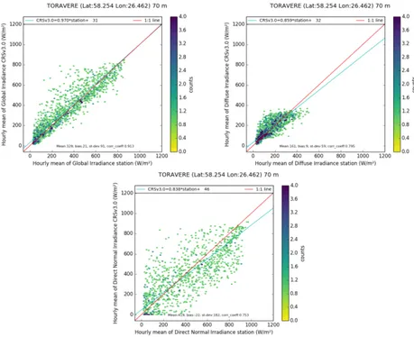
Global Diffuse Direct _{Normal Unit} Mean of measurements at station kept for validation 329 161 419 W/m² Number of data pairs kept for validation 1354 1315 1011 Percentage of data pairs kept relative to the number of data >0 in the period 84.0 81.6 71.5 % Bias (positive means overestimation; ideal value is 0) 21 9 -22 W/m² Bias relative to the mean of measurements 6 5 -5 % RMSE (ideal value is 0) 94 60 183 W/m² RMSE relative to the mean of measurements 28 37 43 % Standard deviation (ideal value is 0) 91 59 182 W/m² Relative standard deviation 27 36 43 % Correlation coefficient (ideal value is 1) 0.913 0.795 0.753

(37)

II. 2-D histograms (scatter density plots) - Histogram of deviations

The 2-D histogram, also known as scatter density plot, indicates how well the estimates given by CRSv3.0 match the coincident measurements on a one-to-one basis. Colors depict the number of occurrence of a given pair (measurement, estimate). In the following, yellow is used for the least frequent pairs, with green for intermediate frequencies and blue for the highest-frequency pairs. Ideally, the dots should lie along the red line. Dots above the red line mean an overestimation. Dots below the red line denote an underestimation. The mean of the measurements, the bias, the standard-deviation and the correlation coefficient are reported. The green line is the affine function obtained by the first axis of inertia minimizing the bias and the standard-deviation. Ideally, this line should overlay the red line. The green line shows the trend in error when values are far off the mean of the measurements.

Figure 1. 2-D histogram between ground measurements (station) and the CRSv3.0 product for Hourly Mean of Irradiance

The histogram of the deviations, or as below the frequency distribution of the deviations, indicates the spreading of the deviations and their asymmetry with respect to the bias. Ideally, frequency should be 100% for deviation equal to 0. The more compact the frequency distribution of the deviations, the better.

(38)

Figure 2. Frequency distribution of the deviations (CRSv3.0 - measurements)

III. Comparison of histograms

The graphs above deal with comparisons of measurements and CRSv3.0 values on a one-to-one basis: for each pair of coincident measurement and CRSv3.0 estimate, a deviation is computed and the resulting set of deviations is analysed.

This section deals with the statistical representativeness of the measurements by CRSv3.0. The frequency distributions of the measurements at station (red line) and the estimates (blue line) are computed and compared. A frequency distribution (histogram) shows how Hourly Mean of Irradiance values are distributed over the whole range of values. Ideally, the blue line should be superimposed onto the red one. If the blue line is above the red one for a given sub-range of values, it means that CRSv3.0 produces these values too frequently. Conversely, if the blue line is below the red one, CRSv3.0 does not produce values in this sub-range frequently enough.

(39)

Figure 3. Frequency distributions of the measurements station (red line) and CRSv3.0 (blue line) for Hourly Mean of Irradiance

IV. Comparison of monthly means and standard deviations

For each calendar month (i.e., Jan, Feb, Mar...) in the selected period, all measurements kept for validation and the coincident CRSv3.0 estimates were averaged to yield the monthly means of Hourly Mean of Irradiance and the standard deviations. The standard-deviation is an indicator of the variability of the radiation within a month, 2017-2017 mixed. In the following graph, monthly means are shown with diamonds and standard deviations as crosses. Red color is for measurements and blue color for CRSv3.0. The closer the blue symbols (CRSv3.0) to the red ones (measurements), the better. A difference between red dot (measurements) and blue diamond (CRSv3.0) for a given month denotes a systematic error for this month: underestimation if the blue diamond is below the red dot, overestimation otherwise. For a given month, a blue cross above the red one means that CRSv3.0 produces too much variability for this month. Conversely, CRSv3.0 does not contain enough variability in the opposite case.

(40)

Figure 4. Monthly means of Hourly Mean of Irradiance measurements at station (red dots) and CRSv3.0 (blue diamonds), and monthly standard-deviation of measurements (red crosses) and CRSv3.0 (blue crosses)

V. Performances in clearness index

V.1. Summary of performances

Summary of the performance of the CRSv3.0 product for Hourly Mean of Clearness Index at TORAVERE

Global Diffuse Direct _{Normal Unit} Mean of measurements at station kept for validation 0.468 0.233 0.317 Number of data pairs kept for validation 1354 1315 1011 Percentage of data pairs kept relative to the number of data >0 in the period 84.0 81.6 71.5 % Bias (positive means overestimation; ideal value is 0) 0.019 0.011 -0.017 Bias relative to the mean of measurements 4 4 -5 % RMSE (ideal value is 0) 0.124 0.081 0.139 RMSE relative to the mean of measurements 26 34 43 % Standard deviation (ideal value is 0) 0.123 0.080 0.138 Relative standard deviation 26 34 43 % Correlation coefficient (ideal value is 1) 0.797 0.543 0.753

(41)

V.2. 2-D histograms (scatter density plots) - Comparison of histograms

Figure 5. 2-D histogram between ground measurements (station) and the CRSv3.0 product for Hourly Mean of Clearness Index

(42)

Figure 6. Frequency distributions of the measurements station (red line) and CRSv3.0 (blue line) for Hourly Mean of Clearness Index

(43)

(44)

Annex. Station ZOSENI

SOLAR RADIATION VALIDATION REPORT

CAMS Radiation Service (CRSv3.0) - Hourly Mean of Irradiance

ZOSENI - Latvia

Latitude: 57.135; Longitude: 25.906; Elevation a.s.l.: 188 m

from 2017-06 to 2017-08

This document reports on the performance of the product CAMS Radiation Service (CRSv3.0) when compared to high quality measurements of solar radiation made at the station of ZOSENI from 2017-06 to 2017-08 using a

standard validation protocol.

Report automatically generated on 2018-03-04 16:12:00

I. Summary of performance

Summary of the performances of the CRSv3.0 product for Hourly Mean of Irradiance at ZOSENI

Global Unit Mean of measurements at station kept for validation 327 W/m² Number of data pairs kept for validation 1301 Percentage of data pairs kept relative to the number of data >0 in the period 84.4 % Bias (positive means overestimation; ideal value is 0) 28 W/m² Bias relative to the mean of measurements 8 %

RMSE (ideal value is 0) 97 W/m²

RMSE relative to the mean of measurements 29 % Standard deviation (ideal value is 0) 92 W/m² Relative standard deviation 28 % Correlation coefficient (ideal value is 1) 0.907

(45)

II. 2-D histograms (scatter density plots) - Histogram of deviations

The 2-D histogram, also known as scatter density plot, indicates how well the estimates given by CRSv3.0 match the coincident measurements on a one-to-one basis. Colors depict the number of occurrence of a given pair (measurement, estimate). In the following, yellow is used for the least frequent pairs, with green for intermediate frequencies and blue for the highest-frequency pairs. Ideally, the dots should lie along the red line. Dots above the red line mean an overestimation. Dots below the red line denote an underestimation. The mean of the measurements, the bias, the standard-deviation and the correlation coefficient are reported. The green line is the affine function obtained by the first axis of inertia minimizing the bias and the standard-deviation. Ideally, this line should overlay the red line. The green line shows the trend in error when values are far off the mean of the measurements.

Figure 1. 2-D histogram between ground measurements (station) and the CRSv3.0 product for Hourly Mean of Irradiance

The histogram of the deviations, or as below the frequency distribution of the deviations, indicates the spreading of the deviations and their asymmetry with respect to the bias. Ideally, frequency should be 100% for deviation equal to 0. The more compact the frequency distribution of the deviations, the better.

CAMS-72 Solar radiation products, Regular Validation Report, J-J-A 2017

HAL Id: hal-01969518

https://hal-mines-paristech.archives-ouvertes.fr/hal-01969518

CAMS-72 Solar radiation products, Regular Validation

Report, J-J-A 2017

Mireille Lefèvre, Lucien Wald

To cite this version:

Copernicus Atmosphere Monitoring Service

D72.2.3.1

Regular Validation Report

Issue #19

J-J-A 2017

CAMS-72

Solar radiation products

Issued by: Armines / M. Lefèvre, L. Wald

Date: 26/03/2018

Contributors

ARMINES

Mireille Lefèvre

Lucien Wald

Table of Contents

1.

Introduction

7

2.

Sources of data and stations

9

2.1 Typical uncertainty of measurements

9

2.2 Definitions of the measured radiation variables

10

2.3 Sources of data

11

2.4 Short description of the stations selected for the validation and maps

12

2.5 List of the stations retained for this quarter

15

3.

Overview of the results

17

3.1 Global irradiance

17

3.2 Diffuse irradiance

19

3.3 Direct irradiance at normal incidence

20

4.

Discussion

22

4.1 Global irradiance

Error! Bookmark not defined.

4.2 Ability to reproduce the intra-day variability

22

4.3 Bias and standard deviation of errors

22

4.4 Ability to reproduce the frequency distributions of measurements

24

4.5 Ability to reproduce the monthly means and standard deviation for the period

26

4.6 Summary

27

5.

Acknowledgements

28

6.

Reference documents

29

Annex A. Procedure for validation

31

1. Taking care of the time system

31

2. Taking care of missing data within an hour or one day

32

3. Computation of deviations and statistical quantities

32

4. Comparison of histograms and monthly means

34

Annex. Station TORAVERE

35

Annex. Station ZOSENI