HAL Id: hal-01091214
https://hal.inria.fr/hal-01091214
Submitted on 4 Dec 2014
HAL is a multi-disciplinary open access
archive for the deposit and dissemination of
sci-entific research documents, whether they are
pub-lished or not. The documents may come from
L’archive ouverte pluridisciplinaire HAL, est
destinée au dépôt et à la diffusion de documents
scientifiques de niveau recherche, publiés ou non,
émanant des établissements d’enseignement et de
RDF
Damian Bursztyn, François Goasdoué, Ioana Manolescu
To cite this version:
Damian Bursztyn, François Goasdoué, Ioana Manolescu. Optimizing Reformulation-based Query
Answering in RDF. [Research Report] RR-8646, INRIA Saclay; INRIA. 2014. �hal-01091214�
0249-6399 ISRN INRIA/RR--8646--FR+ENG
RESEARCH
REPORT
N° 8646
December 2014Reformulation-based
Query Answering in RDF
RESEARCH CENTRE SACLAY – ÎLE-DE-FRANCE
1 rue Honoré d’Estienne d’Orves Bâtiment Alan Turing
Campus de l’École Polytechnique
Damian Bursztyn, François Goasdoué, Ioana Manolescu
Project-Teams OAKSAD
Research Report n° 8646 — December 2014 — 33 pages
Abstract: Reformulation-based query answering is a query processing technique aiming at answering queries under constraints. It consists of reformulating the query based on the constraints, so that evaluating the reformulated query directly against the data (i.e., without considering any more the constraints) produces the correct answer set.
In this paper, we consider optimizing reformulation-based query answering in the setting of ontology-based data access, where SPARQL conjunctive queries are posed against RDF facts on which constraints expressed by an RDF Schema hold. The literature provides query reformulation algorithms for many fragments of RDF. However, reformulated queries may be complex, thus may not be efficiently processed by a query engine; well established query engines even fail processing them in some cases.
Our contribution is (i) to generalize prior query reformulation languages, leading to investigating a space of reformulated queries we call JUCQs (joins of unions of conjunctive queries), instead of a single reformulation; and (ii) an effective and efficient cost-based algorithm for selecting from this space, the reformulated query with the lowest estimated cost. Our experiments show that our technique enables reformulation-based query answering where the state-of-the-art approaches are simply unfeasible, while it may decrease its cost by orders of magnitude in other cases.
Keywords: RDF query answering, SPARQL, query reformulation, query optimization, heuristic algorithms
Résumé : La technique de réponse aux requêtes par reformulation vise à répondre à des requêtes sur des données sous contraintes. Elle consiste de reformuler la requête en fonction des contraintes, de sorte que l’évaluation de la requête reformulée, directement sur les données (c’est-à-dire en ne tenant plus compte des contraintes), produit l’ensemble de réponses correctes. Dans cet article, nous considérons l’optimisation de la réponse aux requêtes par reformula-tion dans le cadre de l’accès aux données au travers d’ontologies, où des requêtes conjonctives SPARQL sont posées sur des faits RDF associés à des contraintes de schéma RDF. La littéra-ture fournit des solutions pour divers fragments de RDF, visant à calculer l’union équivalente de requêtes conjonctives maximalement contenues par rapport aux contraintes. Mais, en général, une telle union est grande et ne peut être efficacement traitée par un moteur de requêtes.
Notre contribution est (i) de généraliser le langage de reformulation de requêtes afin de couvrir un espace de requêtes reformulées équivalentes (au lieu d’avoir une seule reformulation possible), puis (ii) de sélectionner la requête reformulée avec le coût d’évaluation estimée le plus bas. Nos expériences montrent que notre technique permet la réponse aux requêtes par reformulation où les approches sur l’état de l’art sont tout simplement irréalisable, tandis qu’elle peut diminuer leurs coûts de plusieurs ordres de grandeur dans les autres cas.
Mots-clés : Réponse aux requêtes RDF, SPARQL, reformulation de requête, optimisation de requête, algorithme heuristique
1
Introduction
The Resource Description Framework (RDF) [1] is a graph-based data model promoted by the W3C as the standard for Semantic Web applications. As such, it comes with an ontology language, RDF Schema (RDFS), that can be used to enhance the description of RDF graphs, i.e., RDF datasets. The W3C standard for querying RDF graphs is the SPARQL Protocol and RDF Query Language (SPARQL) [2].
Answering SPARQL queries requires to handle the implicit information modeled in RDF graphs, through the essential RDF reasoning mechanism called RDF entailment. Query answers are defined based on both the explicit and the implicit content of an RDF graph. Thus, ignoring implicit information leads to incomplete answers [2].
Two main methods exist for answering SPARQL queries against RDF graphs, both of which consists of a reasoning step, either on the graphs or on queries, followed by a query evaluation step. A popular reasoning method is graph saturation (a.k.a. closure). This consists of pre-computing and adding to an RDF graph all its implicit information, to make it explicit. Answering queries through saturation, then, amounts to evaluating the queries on the saturated graph. While saturation leads to efficient query processing, it requires time to be computed, space to be stored, and must be recomputed upon updates. The alternative reasoning step is query reformulation. This consists in turning a query into a reformulated query, which, evaluated against a non-saturated RDF graph, yields the exact answers to the original query. Since reformulation takes place at query time, it is intrinsically robust to updates; the query reformulation process in itself is also typically very fast, since it only operates on the query, not on the data. However, reformulated queries are often syntactically more complex than the original ones, thus their evaluation may be costly or even unfeasible.
Saturation-based query answering has been well studied by now; efficient saturation algorithms have been proposed, including incremental ones [3, 4, 5, 6]. Most RDF data management systems use saturation-based query answering, either by providing such a reasoning service on RDF graphs, like 3store, OWLIM, Sesame, etc., or by simply assuming that RDF graphs have been saturated prior to loading. Most systems built on top of relational data management systems (RDBMSs, in short) or RDBMS-style engines [7, 8, 9] fall in this category.
Reformulation-based query answering has also been the topic of many works [6, 10, 11, 12, 13], including ours [4, 14, 15]. Existing techniques apply to the Description Logics (DL) [16] fragment of RDF, the conjunctive subset of SPARQL subset and extensions thereof [10, 11, 14, 15, 17, 18, 19], including the “database fragment” of RDF we introduced in [4], the most expressive RDF fragment to date. Only a few RDF data management systems, such as AllegroGraph, Stardog or Virtuoso, use reformulation, in some cases incomplete. The main reason is that state-of-the-art techniques produce reformulated queries whose evaluation is inefficient. A query is typically reformulated into an equivalent large union of conjunctive queries (UCQ), maximally contained in the original query w.r.t. the RDF Schema constraints [4, 6, 10, 11, 12, 14, 15, 17, 18], or in languages for which no well established off-the-shelf query engine exists, such as nested SPARQL [19]. The technique of [13], when translated to the RDF setting, reformulates a conjunctive query into a so-called semi-conjunctive query (SCQ), which is a join of unions of atomic queries. While in many cases this performs better than the UCQ reformulations used in prior work, we show that the reformulation of [13] is only another point in a space, in which we automatically identify the most efficient alternative. Finally, a mix of saturation- and reformulation-based query answering has been investigated in [11]. Only RDF Schema contraints are saturated (thus need maintenance), which allows to avoid generating as part of the reformulation, empty-answer subqueries. This may reduce its syntactic size, but (depending on the ability of the underlying engine to detect empty-answers queries early on) the resulting reformulated query may still be
qref
c(qref)
Query q, RDF data and constraints,
CQto UCQ reformulation algorithm qref
q1 c(q1) ≡ qbest c(qbest) ≡ qn c(qn) ≡ . . . ≡ . . . ≡ qbest Query
optimizer Executionengine
Results
Query evaluation engine (σ, π, ⊲⊳, ∪)
Figure 1: Outline of our approach for efficiently evaluating reformulated SPARQL conjunctive queries.
hard to evaluate.
This work focuses on optimizing reformulation-based query answering in RDF.
We consider the setting in which conjunctive queries (CQ), once reformulated into unions of conjunctive queries (UCQ) or semi-conjunctive queries (SCQ), are handled for evaluation to a query evaluation engine, which can be an RDBMS, a dedicated RDF storage and query processing engine, or more generally any system capable of evaluating selections, projections, joins and unions. As our experiments show, the evaluation of reformulated queries may be very challenging even for well-established relational or native RDF processors, which may handle them inefficiently or simply fail to handle them, even on moderate-size datasets.
The approach we take is the following. Given a SPARQL conjunctive query q and a query reformulation algorithm A which turns a CQ into a UCQ, we explore a novel, large space of alternative reformulations of q that we term JUCQ (for joins of unions and conjunctive queries, and pick the JUCQ reformulation with the lowest estimated cost. Each JUCQ reformulation is obtained based on a carefully chosen set of invocations of the algorithm A, guided by our cost model.
Contributions. The contributions we bring to the problem of efficiently answering SPARQL queries, through reformulation, can be outlined as follows (see Figure 1):
1. We generalize the query reformulation approach, by considering a large space of alternative (equivalent) JUCQ reformulations. This space corresponds to the yellow-background box in Figure 1; it includes and significantly generalizes the prior works based on UCQ or SCQ reformulation. We characterize the size of our space of alternatives, and show that it is oftentimes too large to be completely explored.
2. We define a cost model for estimating the evaluation performance of our reformulated queries through a relational engine; other functions can be used instead, and we show that an RDBMSs’ internal cost model can easily be used, too.
3. We devise a novel algorithm which selects one alternative reformulated query, namely qbest
in Figure 1, which (i) computes the same result as the UCQ reformulated query qref, and
(ii) reduces significantly the query evaluation cost (or simply makes it possible when eval-uating the plain reformulation fails!)
4. We implemented this algorithm and deployed it on top of three well-established RDBMSs, which we show differ significantly in their ability to handle UCQ and SCQ reformulations pro-posed in the previous work. Our experiments confirm that our algorithm makes the most out of each of these engines by leveraging their strengths and avoiding their weaknesses thanks to the usage of our cost model, which we calibrate separately for each system. This makes reformulation feasible when UCQ and/or SCQ fail, and brings performance improve-ments of several orders of magnitude w.r.t. UCQ.
Assertion Triple Relational notation
Class srdf:type o o(s)
Property s p o p(s, o)
Constraint Triple OWA interpretation
Subclass srdfs:subClassOf o s⊆ o Subproperty srdfs:subPropertyOf o s⊆ o
Domain typing srdfs:domain o Πdomain(s) ⊆ o
Range typing srdfs:range o Πrange(s) ⊆ o
Figure 2: RDF (top) & RDFS (bottom) statements.
by comparing it against saturation-based query answering, both based on PostgreSQL and through the dedicated Semantic Web data management platform Virtuoso. These experiments confirm the robustness and performance of our technique, showing in particular that in some cases its performance approaches that of saturation-based query answering. In the sequel, Section 2 introduces RDF, SPARQL conjunctive queries, query reformulation and the performance issues raised by the evaluation of reformulated queries. Section 3 charac-terizes our solution search space and formalizes our problem statement. In Section 4, we present our cost model and solution search space exploration technique, which we evaluate through experiments in Section 5. We discuss related work in Section 6, then we conclude.
2
Preliminaries
In Section 2.1 we introduce RDF graphs, modeling RDF datasets. Section 2.2 presents the SPARQL conjunctive queries, a.k.a. Basic Graph Pattern queries. In Section 2.3, we recall the query reformulation algorithm from [4] used in the present work, chosen because the RDF fragment it applies to is the largest known to date. However, as previously explained, our optimization technique can use any CQ to UCQ reformulation algorithm among those applicable to RDF.
2.1
RDF Graphs
An RDF graph (or graph, in short) is a set of triples of the form s p o. A triple states that its subject s has the property p, and the value of that property is the object o. We consider only well-formed triples, as per the RDF specification [1], using uniform resource identifiers (URIs), typed or un-typed literals (constants) and blank nodes (unknown URIs or literals).
Blank nodes are essential features of RDF allowing to support unknown URI/literal tokens. These are conceptually similar to the variables used in incomplete relational databases based on V-tables [20, 21], as shown in [4].
Notations. We use s, p, o and _:b in triples as placeholders. Literals are shown as strings between quotes, e.g., “string”. Finally, the set of values – URIs (U), blank nodes (B), and literals (L) – of an RDF graph G is denoted Val(G).
Figure 2 (top) shows how to use triples to describe resources, that is, to express class (unary relation) and property (binary relation) assertions. The RDF standard [1] provides a set of built-in classes and properties, as part of the rdf: and rdfs: pre-defined namespaces. We use these namespaces exactly for these classes and properties, e.g., rdf:type specifies the class(es) to which a resource belongs.
Example 1 (RDF graph) The RDF graph G below comprises information about a book, iden-tified by doi1: its author (a blank node _:b1 related to the author name, which is a literal), title
and date of publication.
G=
{doi1 rdf:type Book,
doi1 writtenBy _:b1,
doi1 hasTitle “Game of Thrones”,
_:b1 hasName “George R. R. Martin”,
doi1 publishedIn “1996”}
RDF Schema. A valuable feature of RDF is RDF Schema (RDFS) that allows enhancing the descriptions in RDF graphs. RDFS triples declare semantic constraints between the classes and the properties used in those graphs.
Figure 2 (bottom) shows the allowed constraints and how to express them; domain and range denote respectively the first and second attribute of every property. The RDFS constraints (Fig-ure 2) are interpreted under the open-world assumption (OWA) [20]. For instance, given two rela-tions R1, R2, the OWA interpretation of the constraint R1⊆ R2is: any tuple t in the relation R1
is considered as being also in the relation R2(the inclusion constraint propagates t to R2). More
specifically, when working with the RDF data model, if the triples hasFriend rdfs:domain Person and Anne hasFriend Marie hold in the graph, then so does the triple Anne rdf:type Person. The latter is due to the rdfs:domain constraint in Figure 2.
RDF entailment. Implicit triples are an important RDF feature, considered part of the RDF graph even though they are not explicitly present in it, e.g., Anne rdf:type Person above. W3C names RDF entailment the mechanism through which, based on a set of explicit triples and some entailment rules, implicit RDF triples are derived. We denote by ⊢i
RDF immediate entailment,
i.e., the process of deriving new triples through a single application of an entailment rule. More generally, a triple s p o is entailed by a graph G, denoted G ⊢RDF s p o, if and only if there is a
sequence of applications of immediate entailment rules that leads from G to s p o (where at each step of the entailment sequence, the triples previously entailed are also taken into account). Example 2 (RDFS) Assume that the RDF graph G in Example 1 is extended with the following constraints.
doi1 Book Publication “Game of Thrones” _:b1 “George R. R. Martin” “1996” Person writtenBy hasAuthor publishedIn rdfs:subClassOf rdfs:domain rdfs:range rdfs:subPropertyOf hasTitle writtenBy hasName rdf:type rdf:type hasAuthor rdf:type rdfs:domain rdfs:range
Figure 3: Sample RDF graph.
• books are publications:
Book rdfs:subClassOf Publication
• writing something means being an author: writtenBy rdfs:subPropertyOf hasAuthor • books are written by people:
writtenBy rdfs:domain Book writtenBy rdfs:range Person
The resulting graph is depicted in Figure 3. Its implicit triples are those represented by dashed-line edges.
Saturation. The immediate entailment rules allow defining the finite saturation (a.k.a. closure) of an RDF graph G, which is the RDF graph G∞defined as the fixed-point obtained by repeatedly
applying ⊢i
RDF rules on G.
The saturation of an RDF graph is unique (up to blank node renaming), and does not contain implicit triples (they have all been made explicit by saturation). An obvious connection holds between the triples entailed by a graph G and its saturation: G ⊢RDF s p oif and only if s p o ∈ G∞.
RDF entailment is part of the RDF standard itself; in particular, the answers to a query posed on G must take into account all triples in G∞, since the semantics of an RDF graph is its
saturation [2].
2.2
BGP Queries
We consider the well-known subset of SPARQL consisting of (unions of) basic graph pattern (BGP) queries, modeling the SPARQL conjunctive queries. Subject of several recent works [4, 22, 23, 24], BGP queries are the most widely used subset of SPARQL queries in real-world applications [24]. A BGP is a set of triple patterns, or triples/atoms in short. Each triple has a subject, property and object, some of which can be variables.
Notations. In the following we use the conjunctive query notation q(¯x):- t1, . . . , tα, where
{t1, . . . , tα} is a BGP; the query head variables ¯x are called distinguished variables, and are a
subset of the variables occurring in t1, . . . , tα; for boolean queries ¯x is empty. The head of q is
q(¯x), and the body of q is t1, . . . , tα. We use x, y, z, etc. to denote variables in queries. We
denote by VarBl(q) the set of variables and blank nodes occurring in the query q.
Query evaluation. Given a query q and an RDF graph G, the evaluation of q against G is:
q(G) = {¯xµ| µ : VarBl(q) → Val(G) is a total assignment such that tµ1 ∈ G, t µ
where we denote by tµ the result of replacing every occurrence of a variable or blank node
e ∈ VarBl(q) in the triple t, by the value µ(e) ∈ Val(G).
Note that evaluation treats the blank nodes in a query exactly as it treats non-distinguished variables [25]. Thus, in the sequel, without loss of generality, we consider queries where all blank nodes have been replaced by (new) distinct non-distinguished variables.
Query answering. The evaluation of q against G uses only G’s explicit triples, thus may lead to an incomplete answer set. The (complete) answer set of q against G is obtained by the evaluation of q against G∞, denoted by q(G∞).
Example 3 (Query answering) The following query asks for the names of authors of books somehow connected to the literal 1996:
q(x3):- x1 hasAuthor x2, x2 hasName x3, x1 x4 “1996”
Its answer against the graph in Figure 3 is q(G∞) = {h“George R. R. Martin”i}. The answer
results from G ⊢RDF doi1 hasAuthor _:b1 and the assignment µ = {x1← doi1, x2 ← _:b1, x3 ←
“George R. R. Martin”, x4 ← publishedIn}. Observe that evaluating q directly against G leads
to the empty answer, which is obviously incomplete.
2.3
Query answering against RDF databases
The database (DB) fragment of RDF [4] is, to the best of our knowledge, the most expressive RDF fragment for which both saturation- and reformulation-based RDF query answering has been defined and practically experimented. The fragment is thus named due to the fact that query answering against any graph from this fragment, called an RDF database, can be easily implemented on top of any RDBMS. This DB fragment is defined by:
• Restricting RDF entailment to the RDF Schema constraints only (Figure 2), a.k.a. RDFS entailment. Consequently, the DB fragment focuses only on the application domain knowl-edge, a.k.a. ontological knowlknowl-edge, and not on the RDF meta-model knowledge which mainly begets high-level typing of subject, property and object values found in triples with abstract RDF built-in classes, e.g., rdf:Resource, rdfs:Class, etc.
• Not restricting RDF graphs in any way. In other words, any triple allowed by the RDF specification is also allowed in the DB fragment.
Saturation-based query answering amounts to precomputing the saturation of a database db using its RDFS constraints in a forward-chaining fashion, so that the evaluation of every incoming query q against the saturation yields the correct answer set [4]: q(db∞) = q(Saturate(db)). This
technique follows directly from the definitions in Section 2.1 and Section 2.2, and the W3C’s RDF and SPARQL recommendations.
Reformulation-based query answering, in contrast, leaves the database db untouched and reformulates every incoming query q using the RDFS constraints in a backward-chaining fashion, Reformulate(q, db) = qref, so that the relational evaluation of this reformulation against the (non-saturated) database yields the correct answer set [4]: q(db∞) = qref(db). The Reformulate
algorithm, introduced in [23] and extended in [4], exhaustively applies a set of 13 reformulation rules. Starting from the incoming BGP query q to answer against db, the algorithm produces a union of BGP queries retrieving the correct answer set from the database, even if the latter is not saturated.
Example 4 (Query reformulation) The reformulation of q(x, y):- x rdf:type y w.r.t. the database db(obtained from the RDF graph G depicted in Figure 3), asking for all resources and the classes to which they belong, is:
Triple #answers #reformulations #answers after reformulation (t1) 18, 999, 082 188 33, 328, 108
(t2) 0 4 3, 223
(t3) 396 3 683
Table 1: Characteristics of the sample query q1.
(0) q(x, y):- x rdf:type y ∪ (1) q(x, Book):- x rdf:type Book ∪ (2) q(x, Book):- x writtenBy z ∪ (3) q(x, Book):- x hasAuthor z ∪ (4) q(x, Publication):- x rdf:type Publication ∪ (5) q(x, Publication):- x rdf:type Book ∪ (6) q(x, Publication):- x writtenBy z ∪ (7) q(x, Publication):- x hasAuthor z ∪ (8) q(x, Person):- x rdf:type Person ∪ (9) q(x, Person):- z writtenBy x ∪ (10) q(x, Person):- z hasAuthor x
The terms (1), (4) and (8) result from (0) by instantiating the variable y with classes from db, namely {Book, Publication, Person}. Item (5) results from (4) by using the subclass constraint between books and publications. (2), (6) and (9) result from their direct predecessors in the list, and are due to the domain and range constraints. Finally, (3), (7) and (10) result from their direct predecessors and the sub-property constraint present in the database.
Evaluating this reformulation against db returns the same answer as q(G∞), i.e., the answer
set of q.
3
Optimized reformulation
We first introduce, by examples, the performance issues raised by the evaluation of state-of-the-art reformulated queries. We then introduce our novel reformulation search space and formalize our optimization problem.
Motivating Example 1 Consider the three triples query q1 shown below:
q1(x, y) :- x rdf:type y, (t1)
x ub:degreeF rom “http : //www.U niv532.edu”, (t2)
x ub:memberOf “http : //www.Dept1.U niv7.edu” (t3)
Table 1 gives some intuition on the difficulty of answering q1 over an 108 triples LUBM [26]
benchmark dataset:
The state-of-the-art CQ to UCQ reformulation-based query answering needs to evaluate a refor-mulated query q′
1, which is a union of 2, 256 conjunctive queries, each of which consists of three
triples (one for the reformulation of each triple in the original q1). This query appears in Table
2, where all the triples t1, t2, t3are reformulated together by a CQ to UCQ reformulation algorithm
denoted (.)ref. Observe that in q′
1, many sub-expressions are repeated; for instance, the join over
the single triples resulting from the reformulation of triples (t2) and (t3) will appear for each of
the 188 reformulations of triple (t1). Evaluating q′1 on the 100 million triples LUBM dataset
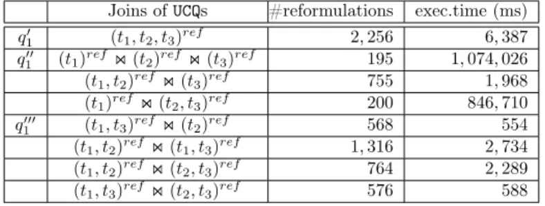
takes more than 6 seconds, in the same experimental setting. Alternatively, one could consider the equivalent query q′′
1 = (t1)ref ⊲⊳ (t2)ref ⊲⊳ (t3)ref, which
joins the CQ to UCQ reformulation of each query’s triple. In other terms, q′′
Joins of UCQs #reformulations exec.time (ms) q′
1 (t1, t2, t3)ref 2, 256 6, 387
q′′
1 (t1)ref⋊⋉ (t2)ref⋊⋉ (t3)ref 195 1, 074, 026
(t1, t2)ref⋊⋉ (t3)ref 755 1, 968 (t1)ref⋊⋉ (t2, t3)ref 200 846, 710 q′′′ 1 (t1, t3)ref⋊⋉ (t2)ref 568 554 (t1, t2)ref⋊⋉ (t1, t3)ref 1, 316 2, 734 (t1, t2)ref⋊⋉ (t2, t3)ref 764 2, 289 (t1, t3)ref⋊⋉ (t2, t3)ref 576 588
Table 2: Sample reformulations of q1.
Triple #answers #reformulations #answers after reformulation (t1) 18, 999, 082 188 33, 328, 108 (t2) 18, 999, 082 188 33, 328, 108 (t3) 476 1 476 (t4) 509 1 509 (t5) 7, 299, 701 3 7, 803, 096 (t6) 7, 299, 701 3 7, 803, 096
Table 3: Characteristics of the sample query q2.
each triple (into, respectively, a union of 188, 4, and 3 queries), and then joins these unions. This query corresponds to the simple semi-conjunctive queries (SCQ) alternative proposed in [13]. While this avoids the repeated work, its performance is much worse: it takes about 1074 seconds to evaluate.
Let us now consider the following equivalent query q′′′
1 = (t1, t3)ref ⊲⊳ (t2)ref where t1, t2, t3
are the triples of the query q1. Evaluating q′′′1 in the same experimental setting takes 554 ms,
more than 10 times faster than the initial reformulation. The performance improvement of q′′′
1 over q′′1 is due to the intelligent grouping of the triples t1 and t3 together. Such grouping of
triples reduce the cardinality of the respective reformulated queries. Thus, (t1, t3)ref has 2, 045
answers and 564 reformulations. Table 2 shows the number of reformulations and execution time for all the eight possible combinations of triples.
Motivating Example 2 Consider now the six triples query q2 shown below:
q2(x, u, y, v, z) :- x rdf:type u, (t1)
y rdf:type v, (t2)
x ub:mastersDegreeF rom “http : //www.U niv532.edu”,(t3)
y ub:doctoralDegreeF rom “http : //www.U niv532.edu”,(t4)
x ub:memberOf z (t5)
y ub:memberOf z (t6)
Statistics on the query triples, when evaluated over a 100 million triples LUBM dataset, appear in Table 3. The CQ to UCQ reformulation of q2, on the other hand, leads to a query q2′
corresponding to a union of 318, 096 six triples queries. Due to its complexity, q′
2 could not be
evaluatedin the same experimental setting1
.
1
Concretely, a stack depth limit exceeded error was thrown by the DBMS. Further, other queries presented I/O exceptions thrown by the DBMS, in connection with a failed attempt to materialize an intermediary result. While it may be possible to tune some parameters to make the evaluation of such queries possible, the same error was raised by many large-reformulation queries, a signal that their peculiar shape is problematic.
Now consider the query q′′
2 = (t1)ref ⊲⊳ (t2)ref ⊲⊳ (t3)ref ⊲⊳ (t4)ref ⊲⊳ (t5)ref ⊲⊳ (t6)ref,
where t1, . . . , t6 are the triples of q2; again, this corresponds to the SCQ reformulation proposed
in [13]. q′′
2 is equivalent to qref2 , and in the same experimental setting, it is evaluated in 229
seconds. This is due to the large results of the (syntactically smal) subqueries (t1)ref, . . . , (t6)ref
(especially the first two, each with 33, 328, 108 results), which required some time to join. Finally, consider the query q′′′
2 = (t1, t3)ref ⊲⊳ (t3, t5)ref ⊲⊳ (t2, t4)ref ⊲⊳ (t4, t6)ref, also
equivalent to q′
2. Evaluating q′′′2 takes 524 ms, more than 430 times faster than one-triple
reformulation. As in the previous example, q′′′
2 gains over q′′2 by first, reducing repeated work, and
second, intelligently grouping triples so that the query corresponding to each triple group can be efficiently evaluated and returns a result of manageable size. In particular, the biggest-size triples (t1) and (t2) had been grouped with (t3) and (t4) respectively, resulting in smaller intermediate
results of 2, 296 and 2, 475 rows respectively, and improving the perfomance. Grouping triples (t3) and (t4) with the (t5) and (t6) respectively, yields analogous performance improvements.
As the above examples illustrate, generalizing the state-of-the-art query reformulation lan-guage of UCQs [4, 6, 10, 11, 12, 14, 15, 17, 18] or of SCQs [13], to that of joins of UCQs, offers a great potential for improving the performance of reformulated queries. We introduce:
Definition 3.1 (JUCQ) A Join of Unions of Conjunctive Queries (JUCQ) is defined as follows: • any conjunctive query (CQ) is a JUCQ;
• any union of CQs (UCQ) is a JUCQ; • any join of UCQs is JUCQ.
In this work, we address the challenge of finding the best-performing JUCQ reformulation of a BGP query against an RDF database, among those that can be derived from a query cover. We define these notions as follows:
Definition 3.2 (JUCQ reformulation) A JUCQ reformulation qJUCQ of a BGP query q w.r.t. a
database db1 is a JUCQ such that qJUCQ(db2) = q(db∞2 ), for any RDF database db2 having the
same schema as db1.
Recall that two RDF databases have the same schema iff their saturations have the same RDFS statements.
BGP query covering is a technique we introduce for exploring a space of JUCQ reformulations of a given query. The idea is to cover a query q with (possibly overlapping) subqueries, so as to produce a JUCQ reformulation of q by joining the (state-of-the-art) CQ to UCQ reformulations of these subqueries, obtained through any reformulation algorithm in the literature (e.g., [4]). Formally:
Definition 3.3 (BGP query cover) A cover of a BGP query q(¯x):- t1, . . . , tn is a set C =
{f1, . . . , fm} of non-empty subsets of q’s triples, called fragments, such thatSmi=1fi= {t1, . . . , tn},
no fragment is included into another, i.e., fi6⊆ fj for 1 ≤ i, j ≤ m and i 6= j, and: if C consists
of more than 1 fragment, then any fragment joins at least with another, i.e., they share a variable. For example, a cover of our query q1 is {{t1, t2}, {t2, t3}}.
Definition 3.4 (Cover queries of a BGP query) Let q(¯x):- t1, . . . , tn be a BGP query and
C = {f1, . . . , fm} one of its covers. A cover query q|fi,1≤i≤mof q w.r.t. C is the subquery whose
body consists of the triples in fi and whose head variables are the distinguished variables ¯x of q
appearing in the triples of fi, plus the variables appearing in a triple of fi that are shared with
For example, the cover {{t1}, {t2, t3}} of our query q1 leads to the cover queries
q1|f1(x, y):- x rdf:type y, and q1|f2(x):- x ub:degreeF rom “http : //www.U niv532.edu”,
x ub:memberOf “http : //www.Dept1.U niv7.edu”.
The theorem below states that evaluating a query q as the join of the cover queries resulting from one of its covers, yields the answer set of q:
Theorem 3.1 (Cover-based reformulation) Let q(¯x):- t1, . . . , tn be a BGP query and C =
{f1, . . . , fm} be any of its covers,
qJUCQ
(¯x):- qUCQ
|f1 ⋊⋉ · · · ⋊⋉ q
UCQ |fm
is a JUCQ reformulation of q w.r.t. any database db, where every qUCQ
|fi is a UCQ reformulation of
the cover query q|fi, for 1 ≤ i ≤ m.
The proof of Theorem 3.1 follows directly from the fact that any cover query q|fi, which is a CQ,
can be equivalently reformulated w.r.t. db into a UCQ qUCQ
|fi, e.g., using any state-of-the-art CQ to
UCQreformulation algorithm.
An upper bound on the size of the cover-based reformulation space for a given query of n triples is given by the number of minimal covers of a set S of n elements [27], i.e., a set of non-empty subsets of S whose union is S, and whose union of all these subsets but one is not S. This bound grows rapidly as the number n of triples in a query’s body increases, e.g., 1 for n = 1, 49 for n = 4, 462 for n = 5, 6424 for n = 6 (http://oeis.org/A046165). In practice, however, we require each fragment to share a variable with another (if any), so that cover queries, hence cover-based reformulations do not feature cartesian products. Therefore, the number of cover-based reformulations is smaller than the number of minimal covers.
In order to select the best performing cover-based reformulation within the above space, we assume given a cost function c which, for a JUCQ q, returns the cost c(q(db)) of evaluating it through an RDBMS storing the database db. Function c may reflect any (combination of) query evaluation costs, such as I/O, CPU etc. As customary, we rely on a cost estimation function cǫ,
which statically provides an approximate value of c. For simplicity, in the sequel we will use c to denote the estimated cost.
The problem we study can now be stated as follows:
Definition 3.5 (Optimization problem) Let db be an RDF database and q be a BGP query against it. The optimization problem we consider is to find a JUCQ reformulation qJUCQ of q
w.r.t. db, among the cover-based reformulations of q with lowest (estimated) cost.
Optimized queries vs. optimized plans. As stated above and illustrated in Figure 1, we seek the best query that is an optimized reformulation of q against db; we do not seek to optimize its plan, instead, we take advantage of existing query evaluation engines for optimizing and executing it. Alternatively, one could have placed this study within an evaluation engine and investigate optimized plans. We comment more the two alternatives in Section 6.
4
Efficient query answering
We present now the ingredients for setting up our cost-based query answering technique. We introduce, in Section 4.1, our cost model for JUCQ reformulation evaluation through an RDBMS. We then provide, in Section 4.2, an exhaustive algorithm that traverses the search space of refor-mulated queries, looking for a cover-based reformulation with lower cost. Finally, in Section 4.3, we introduce a greedy, anytime algorithm that outputs a best query cover of the input BGP query, found so far. This one is then used to evaluate the query as stated by Theorem 3.1.
4.1
Cost model
In this section we detail the cost of evaluating a JUCQ (reformulation) sent to an RDBMS. Such a query is a join of UCQs subqueries of the form: qJUCQ(¯x):- qUCQ
1 ⊲⊳ · · · ⊲⊳ qmUCQ.
The evaluation cost of qJUCQ is
c(qJUCQ
) = cdb+
X
qUCQ i ∈qJUCQ
(ceval(qUCQi ) + cjoin(qUCQi,1≤i≤m) + cmat(qUCQi,1≤i≤m,i6=k)) + cunique(qJUCQ)
(1) reflecting:
(i) the fixed overhead of connecting to the RDBMS cdb;
(ii) the cost to evaluate each of its UCQ sub-queries qUCQ i ;
(iii) the cost of eliminating duplicate rows from each of its UCQ sub-query results; (iv) the cost to join these sub-query results;
(v) the materialization costs: the SQL query corresponding to a JUCQ may have many sub-queries. At execution time, some of these subqueries will have their results materialized (i.e., stored in memory or on disk) while at most one sub-query will be executed in pipeline mode. We assume without loss of generality, that the largest-result sub-query, denoted qUCQ
k ,
is the one pipelined (this assumption has been validated by our experiments so far); and (vi) the cost of eliminating duplicate rows from the result.
In the above, duplicates are eliminated because existing reformulation algorithms (and ac-cordingly, our work) operate under set semantics.
Notations. For a given query q over a database db, we denote by |q|tthe estimated number of
tuples in q’s answer set. Recall that q|{ti} stands for the restriction of q to its i-th triple. Using
the notations above, the number of tuples in the answer set of q|{ti} is denoted |q|{ti}|t.
Duplicate elimination costs. Assuming duplicate elimination is implemented by hashing, we estimate the cost of eliminating duplicate rows from qJUCQ (and qUCQ) as:
cunique(qJUCQ) = cl× |qJUCQ|t
where clis the CPU and I/O effort involved in sorting the results.
When the results are large enough that disk merge sort is needed, we estimate the cost of eliminating duplicate rows from qJUCQ (and qUCQas a particular case) result as:
cunique(qJUCQ) = ck× |qJUCQ|t× log |qJUCQ|t
where ck is the CPU and I/O effort involved in (disk-based) sorting the results.
UCQevaluation costs are estimated by summing up the estimated costs of the CQs: ceval(qiUCQ) = cunique(qiUCQ) +
X
qCQ∈qUCQ i
ceval(qCQ)
The cost of evaluating one conjunctive query ceval(qCQ), where qCQ(¯x):- t1, . . . , tn, through the
RDBMS is made of the scan cost for retrieving the tuples for each of its triples, and the cost of joining these tuples:
ceval(qCQ) = cscan(qCQ) + cjoin(qCQ)
We estimate the scan cost of qCQ to:
cscan(qCQ) = ct×
X
ti∈qCQ
|qCQ |{ti}|t
where ct is the fixed cost of retrieving one tuple.
The join cost of qCQ represents the respective CPU and I/O effort; assuming efficient join
algorithms such as hash- or merge-based etc. are available [28], this cost is linear in the total size of its inputs: cjoin(qCQ) = cj× X ti∈qCQ |qCQ |{ti}|t Therefore, we have: ceval(qiUCQ) = (ct+ cj) × X qCQ∈qUCQ i X ti∈qCQ |qCQ |{ti}|t (2)
UCQjoin cost. As before, we consider the join cost to be linear in the total size of its inputs: cjoin(qi,1≤i≤mUCQ ) = cj×
X qUCQ i X qCQ∈qUCQ i X ti∈qCQ |qCQ |{ti}|t (3)
UCQmaterialization cost. Finally, we consider the materialization cost associated to a query q is cm× |q|tfor some constant cm:
cmat(qUCQi,1≤i≤m,i6=k) = cm×
X qUCQ i ,i6=k X qCQ∈qUCQ i X ti∈qCQ |qCQ |{ti}|t (4) where qUCQ
k is the largest-result sub-query, and the one which is picked for pipelining (and thus
not materialized).
Injecting the equations 2, 3 and 4 into the global cost formula 1 leads to the estimated cost of a given JUCQ. This formula relies on estimated cardinalities of various subqueries of the JUCQ, as well as on the system-dependent constants cdb, cscan, cjoin and cmat, which we
determine by running a set of simple calibration queries on the RDBMS being used. The details are straightforward and we omit them here.
4.2
Exhaustive query cover algorithm (ECov)
As a yardstick for the quality of the query covers we find, we developed an exhaustive query cover finding algorithm, called ECov, that traverses the search space of reformulated queries and outputs a query cover leading to a cover-based reformulation with lowest cost.
Given a BGP query q and a database db, ECov enumerates all the possible query covers, estimates the cost of the corresponding cover-based reformulations, and returns a query cover with the lowest estimated cost. We use this cover as “golden standard”, i.e., the best solutions based on our cost estimation function,
4.3
Greedy query cover algorithm (GCov)
We now present our optimized query cover finding algorithm (GCov). Intuitively, GCov at-tempts to identify query covers such that the estimated evaluation cost of each cover fragment (once reformulated), together with the estimated cost of joining the results of these reformulated fragments, is minimized. Performance benefits in this context are attained from two sources: (i) avoiding the explosion in the size of the reformulated queries that results when many triples, each having many reformulations, are in the same fragment, and (ii) avoiding reformulated frag-ments with very large results, since materialising and joining them is costly. The key intuition for reaching these goals is to include highly selective, few-reformulations triples in several cover fragments. Observe that this is different from (and orthogonal to) join ordering, which the under-lying query evaluation engine (RDBMS in this study) applies independently to each reformulated subquery.
Algorithm 1: Greedy query cover algorithm (GCov) Input : BGP query q(¯x:- t1, . . . , tn), database db
Output: Cover Cbest for the BGP query q 1 C0← {{t1}, {t2}, . . . , {tn}};
2 T ← {t1, t2, . . . , tn};
3 Cbest← C0; moves ← ∅; analysed ← ∅;
4 foreach f ∈ C0, t ∈ T s.t. t 6∈ f ∧ connected(f, {t}) ∧ C0.add(f, t) 6∈ analysed do 5 analysed ← analysed ∪ C0.add(f, t);
6 if C0.add(f, t) est. cost ≤ Cbest est. cost then 7 moves ← moves ∪ (C0, f, t);
8 while moves 6= ∅ do 9 (C, f, t) ← moves.head(); 10 C′ ← C.add(f, t);
11 if C′ est. cost ≤ Cbest est. cost then 12 Cbest← C′;
13 foreach f ∈ C′, t ∈ T s.t. t 6∈ f ∧ connected(f, {t}) ∧ C′.add(f, t) 6∈ analysed do 14 analysed ← analysed ∪ C′.add(f, t);
15 if C′.add(f, t) estimated cost < Cbest estimated cost then 16 moves ← moves ∪ (C′, f, t);
17 return Cbest;
GCov (Algorithm 1) starts with a simple cover C0 consisting of one triple fragments, and
explores possible moves starting from this state. A move consists of adding to one fragment, an extra triple connected to it by at least one join variable, such that the estimated cost associated to the cover-based reformulation thus obtained is smaller than that before the addition. A move may reduce the cost in two ways: (i) by making a fragment more selective, and/or (ii) by leading to the removal of some fragments from the cover. For instance, let {{t1, t2}, {t1, t3}, {t3, t4}} be
a cover of a four-triples query. The move which adds t4to the first fragment, also renders {t3, t4}
redundant. Thus, the cover resulting from the move is: {{t1, t2, t4}, {t1, t3}}. Concretely, all the
fragments of a cover are kept sorted in the decreasing order of their cost. Whenever the cover is updated, we check the fragments from the first to the last; when a fragment is found redundant (with respect to the other fragments in the cover), the fragment is removed.
Possible moves based on the initial cover C0are developed and added to the list moves, sorted
in the increasing order of the estimated cost their bring. Next (line 8), GCov starts exploring possible moves. It picks the most promising one from the sorted moves list and applies it, leading to a new query cover C′. If its estimated cost is smaller than the best (least) cost encountered
so far, the best solution is updated to reflect this C′ (line 12), and possible moves based on C′
are developed and added to the sorted moves list.
GCov explores query covers in breadth-first and greedy fashion, adding to the moves list the possible moves starting from the current best cover, and selecting the next move with smallest cost. In practice, one could easily change the stop condition, for instance to return the best found cover as soon as its cost has diminished by a certain ratio, or after a time-out period has elapsed etc.
5
Experimental evaluation
LUBM q Q01 Q02 Q03 Q04 Q05 Q06 Q07 Q08 Q09 Q10 Q11 Q12 Q13 Q14 Q15 |qref| 136 136 34 564 2 188 156 12 8, 496 13 1 1 2 376 3, 384 |q(db)| (1M) 123 123 41 26, 048 982 5, 537 0 269 0 47, 268 1, 530 88 4, 041 20, 205 0 |q(db)| (100M) 123 123 41 2, 432, 964 92, 026 523, 319 0 269 0 4, 409, 039 142, 337 7, 773 376, 792 1, 883, 960 0 LUBM q Q16 Q17 Q18 Q19 Q20 Q21 Q22 Q23 Q24 Q25 Q26 Q27 Q28 |qref| 2 1 940 2, 444 4 1 1 752 52 156 2, 256 156 318, 096 |q(db)| (1M) 5, 364 5, 388 47, 348 60, 342 228, 086 60, 342 16, 134 100 12 19 5 1 0 |q(db)| (100M) 501, 063 503, 395 4, 425, 553 5, 632, 454 2, 128, 9440 5, 632, 454 1, 510, 695 11, 820 1, 508 1, 463 5 1 495 DBLP q Q01 Q02 Q03 Q04 Q05 Q06 Q07 Q08 Q09 Q10 |qref| 684 292 1, 387 1, 387 4 19 19 1, 721 361 1, 923, 349 |q(db)| 4, 898 16, 424 5, 259, 462 60, 900 19, 576 9, 562 9, 562 203, 462 20 80Table 4: Characteristics of the queries used in our study.
We now present an experimental assessment of our approach. Section 5.1 describes the experimental settings. Section 5.2 studies the effectiveness and efficiency of our optimized reformulation-based query answering technique. Section 5.3 widens our comparison to saturation-based query answering saturation-based on the Postgres RDBMS and the native RDF data management system Virtuoso, then we conclude.
5.1
Settings
Software. We implemented our reformulation-based query answering framework in Java 7, on top of three well-known RDBMSs, namely: PostgreSQL v9.3.2, DB2 Express-C v10.5, and MySQL Community Server v5.6.20. For each RDBMS, we instantiated the cost formulas introduced in Section 4.1 with the proper coefficients, learned by running our calibration queries on that system.
Hardware. All the RDMBSs run on 8-core Intel Xeon (E5506) 2.13 GHz machines with 16GB RAM, using Mandriva Linux release 2010.0 (Official).
Data. We conducted experiments using DBLP (8 million triples) [29] and LUBM [26] with 1 and 100 millions triples.
In our experiments, RDFS constraints are kept in memory, while RDF facts are stored in a Triples(s, p, o) table, indexed by all permutations of the s, p, o columns, leading a total of 6 indexes. Our indexing choice is inspired by [8, 9], to give the RDBMS efficient query evaluation opportunities. Further, as in [4, 8, 9, 23], for efficiency, the Triples(s, p, o) table’s data are dictionary-encoded, using a unique integer for each distinct value (URIs and literals). The dictionary is stored as a separate table, indexed both by the code and by the encoded value. Queries. We used 28 and 10 BGP queries for our evaluation on LUBM and DBLP data sets, respectively. The LUBM queries appear in Tables 5–62
and the DBLP queries in Table 7, while their main characteristics (number of union terms in their UCQ reformulation, denoted |qref|, as
well as the number of results when evaluated on our data sets) are shown in Table 4.
Some queries are modified versions of LUBM benchmark queries, in order to remove redundant triples3
. We designed the others so that (i) they have an intuitive meaning, (ii) they exhibit a variety of result cardinalities, (iii) they exhibit a variety of reformulations, some of which are
2
For readability and without loss of information, the URIs starting with "http://www.lehigh.edu” were slightly shortened by eliminating a few /-separated steps.
3
A query triple is redundant when it can be inferred from the others based on the RDFS constraints. For instance, when looking for x such that x is a person and x has a social security number, if we know that only people have such numbers, the triple “x is a person” is redundant.
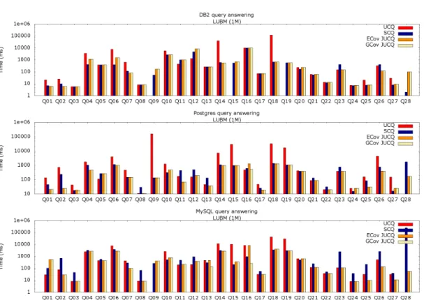
Figure 4: LUBM 1M query answering through UCQ, SCQ, ECov and GCov JUCQ reformulations, against DB2, Postgres and MySQL.
syntactically complex, to allow a study of the performance issues involved and (iv) none of their triples is redundant.
All measured times are averaged over 3 (warm) executions. Moreover, queries whose evalua-tion requires more than 2 hours were interrupted; we point them out when commenting on the experiments’ results.
5.2
Optimized reformulation
In this section, we compare our reformulation-based query answering technique with those from the literature based on UCQs and SCQs.
Effectiveness: is an optimizer needed? The first question we ask is whether exploring the space of JUCQ alternatives is actually needed, or could one just rely on a simple (fixed) query cover?
The UCQ reformulation used in many prior works is a particular case of the JUCQ reformulations we introduced in this work; it corresponds to a cover of a single fragment made of all the query triples (recall q′
1 in Motivating Example 1, Section 3). From a database perspective, it
corresponds to pushing the joins below a single (potentially large) union. At the other extreme, the SCQ reformulation proposed in [13] is a particular case of JUCQ reformulation obtained from a cover where each query triple is alone in a fragment (recall q′′
1 in the same example). The SCQ
reformulation can thus be thought of as pushing all unions below the joins. Both the UCQ and SCQ reformulations correspond to a cover where each triple appears in exactly one fragment, whereas our JUCQs do not have this constraint; further, the UCQ and SCQ reformulations do not take into
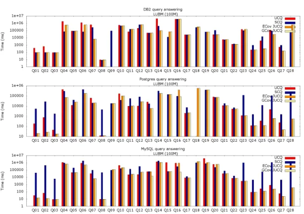
Figure 5: LUBM 100M query answering through UCQ, SCQ, ECov and GCov JUCQ reformulations, against DB2, Postgres and MySQL.
account quantitative information about the data and query.
We compared the performance of query answering through: (i) UCQ reformulation; (ii) SCQ reformulation; (iii) the JUCQ recommended by the exhaustive ECov algorithm; (iv) the JUCQ recommended by our greedy GCov algorithm.
Figures 4 and 5 show the evaluation times for LUBM queries on the 1M and 100M datasets respectively, on the three RDBMSs we tested; observe the logarithmic time axis. Missing bars correspond to executions which timed out or were infeasible (due to the queries’ sizes or to the limited available memory). Figures 4 and 5 show that neither UCQ nor SCQ reformulation are reliable options. Indeed, UCQ is the slowest for many queries on DB2 and Postgres, sometimes by more than an order of magnitude, and it fails for Q9, Q15, Q18 (for LUBM 100M only), Q19
and Q28 on DB2, to which we add Q6, Q14 and Q16 on Postgres (for LUBM 100M). MySQL
fails for queries Q9, Q18 (for LUBM 100M only) and Q28. SCQ is very inefficient on MySQL,
and also on Postgres for Q1, Q2, Q3, Q8and Q23-Q28; it is often the worst choice for MySQL and
Postgres for LUBM 100M. In contrast, the GCov-chosen JUCQ always completes and is the fastest overall in all but Q4, Q6, Q9, Q11, Q15 and Q28 on DB2. As for the query Q9, the covers chosen
by ECov and GCov for DB2 led to a timeout. We studied the respective chosen execution plan and found that in this particular case, the DB2 optimizer made poor decisions; details can be found in the Appendix. This issue could perhaps be solved by further tuning our simple cost model or, even more likely, by making DB2’s own cost model available to our algorithm. We consider this to be out of the scope of the present work, in which our simple cost model already shows an overall good behaviour and robustness w.r.t. our reformulation-based query answering optimization. Figures 4 and 5 also show that the GCov JUCQ performs as well as the ECov
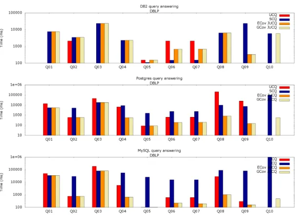
Figure 6: DBLP query answering through UCQ, SCQ, ECov and GCov JUCQ reformulations, against DB2, Postgres and MySQL.
one, thus the greedy is making smart choices. In Figure 5, the GCov JUCQ is up to 4 orders of magnitude faster than the SCQ reformulation and two orders of magnitude faster than UCQ (on LUBM 1M, it wins by 3 orders of magnitude w.r.t. UCQ).
Figure 6 presents similar experiments on the DBLP dataset. It also shows that no fixed reformulation technique is always the best. On DB2, SCQ performs very well for Q6and Q7, and
very poorly for Q9; on the latter, UCQ times out. In contrast, JUCQ performance is robust, the
best in all cases but Q2, Q5, Q6and Q7, and for those it is not very far from the optimum. On
Postgres and MySQL the GCov JUCQ performance is the best in all cases, and more than two orders of magnitude faster than the SCQ and UCQ reformulation. These experiments highlight the interest of the JUCQ reformulation space, and the usefulness of our cost model in guiding ECov and GCov search. Further, in Figure 6, we see that the ECov bar is missing for Q10, on all
systems. This is because on this 10-atoms query, the search space is so large that exhaustive search is unfeasible.
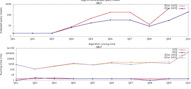
GCov performance We now turn to considering the number of covers: overall (as explored by the exhaustive ECov), and the subset traversed by our greedy GCov; these are depicted in Figure 7 and 8, also in logarithmic scale. (Recall that UCQ and SCQ each correspond to one fixed cover.) While the search space can be very large (e.g., for LUBM Q2, Q9 or Q12), GCov only
explores a small subset of this space. The same figures also show the running time of GCov and ECov, and the time to build the UCQ, respectively the SCQ reformulations (again, observe the logarithmic time axis). The time is spent to: obtain the statistics necessary for estimating the
Figure 7: Number of query covers explored by the algorithms (top) and algorithm running times (bottom) for the LUBM queries.
Figure 8: Number of query covers explored by the algorithms (top) and algorithm running time (bot-tom) for DBLP queries.
number of results of various fragments; reformulate each fragment, estimate its cost, and all other steps shown in Algorithm 1. We see that GCov’s running time may be one order of magnitude less than the one of ECov; as expected, building the (cost-ignorant) UCQ and SCQ is faster, at the expense of their evaluation time when feasible. The highest running time is recorded for queries having a huge UCQ reformulation (LUBM Q28, respectively DBLP Q10, detailed in Table 4), for
which estimating the costs of equivalent JUCQs involves intensive calls to the reformulation and cardinality estimation algorithms. Moreover, for DBLP Q10, ECov times out while exploring
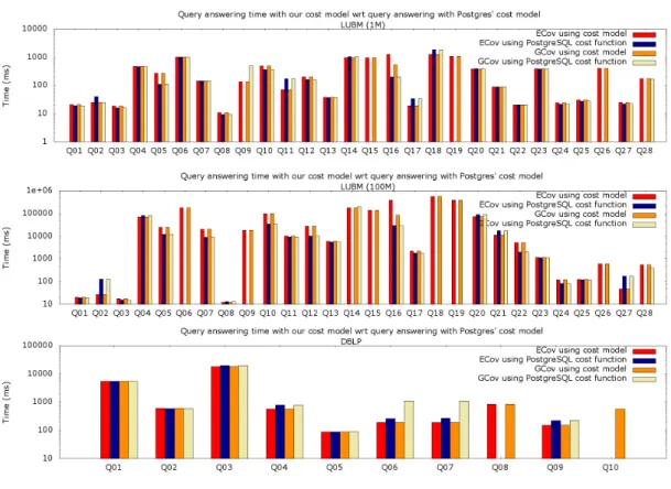
Figure 9: Cost model comparison.
Alternative: using the RDBMS cost estimation The second question we study is the quality of our cost estimation, that is crucial in guiding GCov decisions. The golden standard one can compare against is the RDBMS’s internal cost estimation function: this is because any cover we chose is evaluated by sending it (as a SQL statement) to the system which optimizes it according to its internal cost model. Thus, the cost function used by GCov should be as close as possible to the RDBMS one.
For this comparison, whenever we needed to estimate the cost of a cover, we sent to Postgres an explain statement for the corresponding cover-based reformulation, and extracted from its
result Postgres’ cost estimation4
.
Figure 9 shows the evaluation time of the JUCQ reformulations chosen by ECov and GCov, based on one hand on our cost function, and on the other hand on the Postgres one. Most of the time, the results are similar, demonstrating that our cost model is indeed close to the one of Postgres. In a few cases (LUBM Q5, Q7for 100M only, Q10, Q12, Q16 and Q22for 100M only),
using Postgres’ cost model helped avoid bad ECov/GCov decisions; however, for the LUBM queries Q6, Q9, Q14, Q15, Q18, Q19, Q26and Q28, as well as the DBLP queries Q8and Q10, the
ECov and/or GCov JUCQs chosen based on Postgres’ cost estimation timed out before completing or failed to execute the explain.
Figure 9 demonstrates that our cost model (Section 4.1) has lead, overall, our algorithms to evaluation choices very similar to the those made using Postgres’ cost model, validating its accuracy. Moreover, our cost model provides more robustness than Postgres’ one, as its evaluation
4
Doing this for every examined cover slowed down our search significantly, thus we do not recommend running GCov out of a RDBMS based on the RDBMS’s internal cost model.
choices are always feasible, while those made based on Postgres’ one sometimes fail.
5.3
Comparison with saturation
(a) LUBM 1M dataset query answering through Virtuoso and Postgres.
(b) LUBM 100M dataset query answering through Virtuoso and Postgres.
Figure 10: Query answering through Virtuoso and Postgres (via saturation, respectively, optimized reformulation).
As explained in the Introduction, graph saturation and query reformulation are the two main techniques for answering queries under constraints. Saturation-based query answering can be very efficient, once the data is saturated; however, if the RDF graph is updated, the cost of maintaining the saturation may be very high [4]. In contrast, query reformulation is performed directly at query time, and so it naturally adapts to the current state of the database. The performance trade-off between saturation- and reformulation-based query answering depends on the schema, on the nature of updates, and on the data statistics [4].
In this section, we show how our optimized JUCQ reformulation-based query answering tech-nique impacts the performance comparison with saturation-based query answering. Figure 10 compares on the LUBM 1M and 100M datasets: (i) UCQ reformulation; (ii) saturation-based query answering based on Postgres; (iii) saturation-based query answering based on Virtuoso v6.1.6 (open-source, multi-threaded edition); and (iv) our GCov-chosen JUCQ. As expected, UCQreformulation performs much worse than saturation-based query answering, and worse than the GCov JUCQ by up to three orders of magnitude. Further, Figure 10(b) shows that the un-derlying RDBMS is unable to handle the UCQ reformulation of the queries Q6, Q9, Q14-Q16,
Q18, Q19 and Q28. On some queries, such as Q6, Q15, Q19 or Q23− Q28, saturation keeps its
advantage even compared to our optimized JUCQ reformulation. However, on queries such as Q3− Q5, Q7− Q14, Q16− Q18 and Q20− Q22, the JUCQ reformulation is close to (competitive
with) saturation-based query answering, which is remarkable given that reformulation reasons at query time, and considering the performance gap observed between the two in previous works, e.g., [4].
5.4
Experiment conclusion
Our experiments lead to the following conclusions.
(1). Confirming the intuition given by our example in Section 3, the space of JUCQ reformulation comprises alternative reformulations of a given BGP query w.r.t. the RDFS constraints, whose evaluation is (i) feasible when UCQ reformulation fails, and (ii) up to 4 orders of magnitude more efficient than a fixed reformulation strategy, such as UCQ or SCQ. (2). While ECov is slow for large-reformulation queries, GCov identifies covers leading to efficient reformulations quite fast, confirming the feasibility of our optimized reformulation technique at query time. (3). The cost model on which our search is based performs globally well; in particular, when calibrated for Postgres, we have shown it leads to chosing covers very close to the ones obtained when relying on Postgres’ internal cost model. (4). While saturation-based query answering has reasons to be much more efficient than reformulation techniques (if one is willing to disregard the initial cost of saturating the database, as well as any cost related to saturation maintenance!), our efficient reformulation technique is in many cases competitive with saturation-based query answering, both through a relational server and through the native-RDF Virtuoso server. This confirms the important performance improvement brought by our work to reformulation-based query answering in RDF; recall that any CQ to UCQ reformulation algorithm could be used with our cost-based GCov optimization technique.
6
Related work
The context of our work is the problem of answering conjunctive queries against RDF facts, in the presence of RDFS constraints. As mentioned in the introduction, solutions from the literature rely on RDF graph saturation, on query reformulation, or by mixing both [11]; our work focused on making query answering based on reformulation performant. Below, we position our work w.r.t. these two techniques.
Saturation-based query answering. When using graph saturation, all the implicit triples are computed and explicitly added to the database; query answering then reduces to query evaluation on the saturated database. Well-known SPARQL compliant RDF platforms such as 3store [30], Jena [31], OWLIM [32], Sesame [33], Oracle Semantic Graph [34] support saturation-based query answering, based on (a subset of) RDF entailment rules.
RDF platforms originating in the data management community, such as Hexastore [9] or RDF-3X [8], ignore entailed triples and only provide query evaluation on top of the RDF graph, which is assumed to be already saturated.
Parallel RDF saturation algorithms have been proposed in the literature. In WebPie [35], an RDF graph is stored in a distributed file system and the saturation of the graph is computed using MapReduce jobs. A similar approach, based on C/Message Passing Interface, is presented in [36].
The drawbacks of saturation w.r.t. updates have been pointed out in [3], which proposes a truth maintenance technique implemented in Sesame. It relies on the storage and management of the justifications of entailed triples (which triples beget them). This technique incurs a high overhead of handling justifications when their number and size grow. Therefore, [37] proposes to compute only the relevant justifications w.r.t. an update, at maintenance time. This technique is implemented in OWLIM, however [32] points out that updates upon RDFS constraint deletions can lead to poor performance. More efficient saturation maintenance techniques are provided in [4, 6] based on the number of times triples are entailed.
Reformulation-based query answering. When using query reformulation, a given BGP query is reformulated based on the RDFS constraints into a target language, such that evaluating the reformulated query through an appropriate engine yields the query answer.
UCQ reformulation [4, 6, 10, 11, 12, 14, 15, 17, 18] applies to various fragments of RDF, ranging from the Description Logics (DL) one up to the Database one, the largest for which this technique have been considered so far. UCQ reformulation corresponds in this work to a JUCQ reformulation obtained from a single fragment query cover. SCQ reformulation [13] was defined for the DL fragment of RDF. In our setting, it corresponds to a JUCQ reformulation obtained from a query cover in which each triple is alone in a fragment. Our experiments have shown that the evaluation performance for both UCQ or SCQ reformulation can be very poor.
Among popular RDF data management systems, the only ones supporting reformulation-based query answering are Stardog, Virtuoso (which supports only the rdfs:subClassOf and rdfs:subPropertyOf RDFS rules) and AllegroGraph [38] which supports the four RDFS rules but whose reasoning implementation is incomplete5
. Virtuoso is based on SCQ reformulation, while Stardog uses UCQ reformulation; we found no information about AllegroGraph’s query reformulation language. Nested SPARQL is the target reformulation language in [19]; in contrast, we focus on translating into a commonly supported language such as JUCQs which in turn can be efficiently evaluated by an SQL engine. In [11], the schema is maintained saturated and reformulation is applied at runtime. Our approach could apply in that setting, to improve their reformulation performance.
5
Datalog has also been used as a target reformulation language. For instance, Presto [12, 39] reformulates queries in a DL-Lite setting into non-recursive Datalog programs. These DL-Lite formalisms are strictly more expressive from a semantic constraint viewpoint than the RDFS constraints we consider. Thus, their method could be easily transferred (restricted) to the DL fragment of RDF which, as previously mentioned, is a subset of the database fragment of RDF that we consider. However, these works did not consider cost-driven performance optimization based on data statistics and a query evaluation cost model as in our work.
From a database optimization perspective, the performance advantage we gain by adding selective triples next to very large ones within query covers’ fragments is akin to the semi-join reducers technique, well-known from the distributed database context [40]. It has been shown e.g., in [41] that semi-join reducers can also be beneficial in a centralized context by reducing the overall join effort. In this work, we use a technique reminiscent of semi-joins in order to pick the best query-level formulation of a reformulated query, to make its evaluation possible and efficient; this contrasts with the traditional usage of semi-joins at the level of algebraic plans. On one hand, working at the plan level enables one to intelligently combine traditional joins and semi-joins to obtain the best performance. On the other hand, producing (as we do) an output at the query (syntax) level (recall Figure 1) enables us to take advantage of any existing system, and of its optimizer which will figure out the best way to evaluate such queries, a task at which many systems are good once the query has a "reasonable” shape and size. Further, expressing optimized reformulations as queries allows us not to (re-)explore the search space of join orders etc. together with the (already large) space of possible reformulated queries.
7
Conclusion
Our work is placed in the setting of query answering against RDF graphs in the presence of RDF Schema constraints. In particular, we focus on improving the performance of reformulation-based RDF query answering.
We have identified a space of alternative JUCQ reformulations, whose evaluation (based on a standard, semantics-unaware query processor) may be (i) feasible even when the prominent UCQ reformulation is not, and (ii) more efficient by up to three orders of magnitude. Further, we have presented a cost model for such JUCQ alternatives, and proposed an anytime greedy cost-based algorithm capable of identifying such efficient alternatives. Our technique may be used with any CQ-to-UCQ query reformulation algorithm (recall Figure 1) and thus we consider it a big step forward toward making reformulation-based query answering efficient. This is particularly useful in contexts when the data and/or constraints are updated, and saturation-based techniques incur high maintenance costs as illustrated e.g., in [4]; in contrast, applying at query time, reformulation-based query answering is naturally robust to updates, and (through cost-based techniques such as the one described in our work) close to saturation-based performance but without its drawbacks.
References
[1] “Resource description framework.” http://www.w3.org/RDF.
[2] “SPARQL protocol and RDF query language.” http://www.w3.org/TR/ rdf-sparql-query.
[3] J. Broekstra and A. Kampman, “Inferencing and truth maintenance in RDF Schema: Ex-ploring a naive practical approach,” in PSSS Workshop, 2003.
[4] F. Goasdoué, I. Manolescu, and A. Roatiş, “Efficient query answering against dynamic RDF databases,” in EDBT, 2013.
[5] J. Urbani, S. Kotoulas, J. Maassen, F. van Harmelen, and H. E. Bal, “WebPIE: A web-scale parallel inference engine using MapReduce,” J. Web Sem., vol. 10, pp. 59–75, 2012.
[6] J. Urbani, A. Margara, C. J. H. Jacobs, F. van Harmelen, and H. E. Bal, “Dynamite: Parallel materialization of dynamic RDF data,” in ISWC, 2013.
[7] D. J. Abadi, A. Marcus, S. R. Madden, and K. Hollenbach, “Scalable semantic web data management using vertical partitioning,” in VLDB, 2007.
[8] T. Neumann and G. Weikum, “The RDF-3X engine for scalable management of RDF data,” VLDBJ, vol. 19, no. 1, pp. 91–113, 2010.
[9] C. Weiss, P. Karras, and A. Bernstein, “Hexastore: Sextuple indexing for Semantic Web data management,” PVLDB, 2008.
[10] Z. Kaoudi, I. Miliaraki, and M. Koubarakis, “RDFS reasoning and query answering on DHTs,” in ISWC, 2008.
[11] J. Urbani, F. van Harmelen, S. Schlobach, and H. Bal, “QueryPIE: Backward reasoning for OWL Horst over very large knowledge bases,” in ISWC, 2011.
[12] G. D. Giacomo, D. Lembo, M. Lenzerini, A. Poggi, R. Rosati, M. Ruzzi, and D. F. Savo, “MASTRO: A reasoner for effective ontology-based data access,” in ORE, 2012.
[13] M. Thomazo, “Compact rewriting for existential rules,” IJCAI, 2013.
[14] P. Adjiman, F. Goasdoué, and M.-C. Rousset, “SomeRDFS in the semantic web,” JODS, vol. 8, 2007.
[15] F. Goasdoué, K. Karanasos, J. Leblay, and I. Manolescu, “View selection in semantic web databases,” PVLDB, 2011.
[16] F. Baader, D. Calvanese, D. L. McGuinness, D. Nardi, and P. F. Patel-Schneider, eds., The DL Handbook: Theory, Implem., and Applications, Cambridge Univ. Press, 2003.
[17] D. Calvanese, G. D. Giacomo, D. Lembo, M. Lenzerini, and R. Rosati, “Tractable reasoning and efficient query answering in description logics: The DL-Lite family,” JAR, vol. 39, no. 3, 2007.
[18] G. Gottlob, G. Orsi, and A. Pieris, “Ontological queries: Rewriting and optimization,” in ICDE, 2011. Keynote.
[19] M. Arenas, C. Gutierrez, and J. Pérez, “Foundations of RDF databases,” in Reasoning Web, 2009.
[20] S. Abiteboul, R. Hull, and V. Vianu, Foundations of Databases. Addison-Wesley, 1995. [21] T. Imielinski and W. Lipski, “Incomplete information in relational databases,” JACM,
vol. 31, no. 4, 1984.
[22] M. Stocker, A. Seaborne, A. Bernstein, C. Kiefer, and D. Reynolds, “SPARQL basic graph pattern optimization using selectivity estimation,” in WWW, 2008.
[23] F. Goasdoué, K. Karanasos, J. Leblay, and I. Manolescu, “View selection in semantic web databases,” PVLDB, vol. 5, no. 2, 2011.
[24] F. Picalausa, Y. Luo, G. H. Fletcher, J. Hidders, and S. Vansummeren, “A structural ap-proach to indexing triples,” in ESWC, 2012.
[25] S. Abiteboul, I. Manolescu, P. Rigaux, M.-C. Rousset, and P. Senellart, Web Data Manage-ment. Cambridge University Press, 2011.
[26] Y. Guo, Z. Pan, and J. Heflin, “LUBM: A benchmark for OWL knowledge base systems,” J. Web Sem., vol. 3, no. 2-3, pp. 158–182, 2005.
[27] T. Hearne and C. Wagner, “Minimal covers of finite sets,” Discrete Mathematics, vol. 5, pp. 247–251, 1973.
[28] R. Ramakrishnan and J. Gehrke, Database Management Systems. NY, USA: McGraw-Hill, Inc., 3 ed., 2003.
[29] “DBLP.” http://kdl.cs.umass.edu/data/dblp/dblp-info.html. [30] “3store.” http://www.aktors.org/technologies/3store.
[31] “Apache jena.” http://jena.apache.org. [32] “Owlim.” http://owlim.ontotext.com. [33] “Sesame.” http://www.openrdf.org.
[34] “Oracle semantic graphs.” http://docs.oracle.com/cd/E16655_01/appdev.121/ e17895/toc.htm, 2014.
[35] J. Urbani, S. Kotoulas, E. Oren, and F. van Harmelen, “Scalable Distributed Reasoning using MapReduce,” in ISWC, 2009.
[36] J. Weaver and J. A. Hendler, “Parallel Materialization of the Finite RDFS Closure for Hundreds of Millions of Triples,” in ISWC, 2009.
[37] B. Bishop, A. Kiryakov, D. Ognyanoff, I. Peikov, Z. Tashev, and R. Velkov, “OWLIM: A family of scalable semantic repositories,” Semantic Web, vol. 2, no. 1, 2011.
[38] “AllegroGraph RDFStore Web 3.0 Database.” http://franz.com/agraph/allegrograph, 2014. [39] R. Rosati and A. Almatelli, “Improving query answering over DL-Lite ontologies,” in KR,
[40] M. T. Özsu and P. Valduriez, Principles of Distributed Database Systems, Third Edition. Springer, 2011.
[41] K. Stocker, R. Braumandl, A. Kemper, and D. Kossmann, “Integrating semi-join-reducers into state-of-the-art query processors,” in ICDE, 2001.


![Table 1 gives some intuition on the difficulty of answering q 1 over an 10 8 triples LUBM [26]](https://thumb-eu.123doks.com/thumbv2/123doknet/11364482.285618/12.892.255.588.319.521/table-gives-intuition-difficulty-answering-q-triples-lubm.webp)