HAL Id: dumas-03172217
https://dumas.ccsd.cnrs.fr/dumas-03172217
Submitted on 17 Mar 2021
HAL is a multi-disciplinary open access
archive for the deposit and dissemination of sci-entific research documents, whether they are pub-lished or not. The documents may come from teaching and research institutions in France or abroad, or from public or private research centers.
L’archive ouverte pluridisciplinaire HAL, est destinée au dépôt et à la diffusion de documents scientifiques de niveau recherche, publiés ou non, émanant des établissements d’enseignement et de recherche français ou étrangers, des laboratoires publics ou privés.
Bioenergetic modeling of the variability of life history
traits for anchovy and sardine between the Gulf of Lion,
the Bay of Biscay and the English Channel
Clara Menu
To cite this version:
Clara Menu. Bioenergetic modeling of the variability of life history traits for anchovy and sardine between the Gulf of Lion, the Bay of Biscay and the English Channel. Life Sciences [q-bio]. 2020. �dumas-03172217�
Modélisation bioénergétique de la variabilité
des traits d’histoire de vie de l’anchois et de la
sardine entre le golfe du Lion, le golfe de
Gascogne et la Manche
Par : Clara MENU
Soutenu à Rennes le 16 septembre 2020
Devant le jury composé de : Président : Didier GASCUEL Maître de stage : Martin HURET Enseignant référent : Didier GASCUEL
Autres membres du jury (Nom, Qualité)
Etienne RIVOT (Enseignant-chercheur, Agrocampus Ouest)
Marie SAVINA-ROLLAND (Chercheuse, Ifremer STH-LTBH)
Les analyses et les conclusions de ce travail d'étudiant n'engagent que la responsabilité de son auteur et non celle d’AGROCAMPUS OUEST
Ce document est soumis aux conditions d’utilisation
«Paternité-Pas d'Utilisation Commerciale-Pas de Modification 4.0 France» AGROCAMPUS OUEST
CFR Angers CFR Rennes
Année universitaire : 2019 - 2010 Spécialité :
Ingénieur agronome
Spécialisation (et option éventuelle) : Sciences Halieutiques et Aquacoles (Ressources et Ecosystèmes Aquatiques)
Mémoire de fin d’études
■ d'ingénieur de l'École nationale supérieure des sciences agronomiques, agroalimentaires, horticoles et du paysage (AGROCAMPUS OUEST), école interne de l'institut national d'enseignement supérieur pour l'agriculture, l'alimentation et l'environnement
☐ de master de l'École nationale supérieure des sciences agronomiques,
agroalimentaires, horticoles et du paysage (AGROCAMPUS OUEST), école interne de l'institut national d'enseignement supérieur pour l'agriculture, l'alimentation et l'environnement
Remerciements
Je souhaite remercier tout l’équipe de LBH qui m’a accueillie pendant ces six mois de stage, malgré une période de confinement absolument interminable. Merci à Aurore, Hervé, Sophie, Jérôme, Christophe, Martial et Mathieu pour leur bienveillance et les pauses café ponctuées de boules choco et de blagues en tout genre.
Merci à Jeroen Van der Kooij, Mathieu Doray et Tarek Hattab qui ont été nos experts locaux dans cette étude et qui nous ont permis d’obtenir les données de campagnes ainsi qu’un regard extérieur, en particulier pour la Méditerranée.
Merci également à Laure Pecquerie et Cédric Bacher qui m’ont aidé pour la préparation des oraux, qui ne sont clairement pas mon point fort, et avec qui nous allons poursuivre l’étude des petits pélagiques.
Merci en particulier à Chloé qui m’a toujours proposé son aide, autant au boulot qu’à la découverte de Brest ! Bon courage pour cette fin de thèse, promis tu auras des brownies pour maintenir ton moral à flots et faire en sorte que ta coloc survive !
Un grand merci à Martin qui a toujours été disponible, au bureau, en télétravail et même pendant ses congés. Tu as été d’une grande aide et ce, malgré tes expressions nordistes qui restent totalement incompréhensibles, en particulier quand vous vous y mettez à deux avec Chloé. . .
Ce stage marque surtout la fin de très belles années à l’agro. Un grand merci à la promo 167 pour ces moments partagés ensemble, merci à la bran’loc de m’avoir accueillie pendant ma période sans-abris et merci aux halieutes qui ont toujours su passer de la salle info à la piste avec une agilité déconcertante.
Une pensée particulière pour la team pause, Taron, Hugo, Micka, Christelle et Ilan, qui ont toujours été présents pour affronter le temps breton ou partir en quête de pièces pour la machine à café.
Merci à tous pour ces années rennaises inoubliables qui m’auront permis de devenir, un génie avant d’être ingénieur.
Contents
RemerciementsList of Acronyms, Tables, Figures and Appendices
1 Introduction 1
1.1 Rapid population dynamics of small pelagic fish in response to environment
and fishery . . . 1
1.2 A general decrease in size and body condition . . . 2
1.3 Small pelagic fish growth in relation to the environment . . . 3
1.4 Objective of this study . . . 4
2 Material and method 6 2.1 Dynamic Energy Budget . . . 6
2.1.1 Dynamic Energy Budget theory . . . 6
2.1.2 Adjustments for small pelagics . . . 9
2.2 Fish data . . . 10
2.2.1 Larvae and juveniles . . . 10
2.2.2 Adults . . . 10
2.2.3 Exploration of the observed spatio-temporal variability . . . 11
2.3 Environmental forcing variables . . . 11
2.3.1 POLCOMS-ERSEM . . . 11
2.3.2 Data extraction . . . 11
2.3.3 Comparison of POLCOMS-ERSEM with satellite data . . . 12
2.3.4 Spatio-temporal variability of the environmental variables . . . 12
2.4 DEB calibration . . . 13
2.5 Environmental based scenarios . . . 14
2.5.1 Improving temporal trends . . . 14
2.5.2 Improving spatialization for anchovy . . . 14
3 Results 16 3.1 Decrease in length and weight at adult stage . . . 16
3.2 Environment characteristics . . . 17
3.2.1 Comparisons between POLCOMS-ERSEM and satellite data . . . . 17
3.2.2 Low temporal variability in the environment . . . 18
3.2.3 Spatial variability in the environments . . . 20
3.3 DEB model . . . 21
3.3.1 New estimation of parameters . . . 21
3.3.2 Model fit . . . 21
3.4 Energy allocation . . . 24
3.5 Environmental scenarios . . . 26
3.5.1 No significant differences while improving temporal trends . . . 26
3.5.2 Larger weight variations while improving spatialization for anchovies 26 4 Discussion 28 4.1 DEB modelling allows to explain part of the spatial variability of traits . . 28
4.1.1 A comprehensive modelling framework . . . 28
4.1.3 Energy condition . . . 28
4.2 Why does the environment not transcribe the temporal variability of traits ? 29 4.2.1 Lack of temporal variability in the environmental variables . . . 29
4.2.2 Changes in zooplankton communities . . . 30
4.2.3 Improving modelling scale . . . 31
4.3 Calibration and genetic adaptation . . . 32
4.4 Fishing, another possible pressure . . . 32
5 Conclusion 33
References 34
List of Acronyms
BoB : Bay of BiscayCEFAS : Centre for Environment, Fisheries and Aquaculture Science DEB : Dynamic Energy Budget
EC : English Channel
ERSEM : European Regional Seas Ecosystem Model GoL : Gulf of Lion
IFREMER : French Research Institute for Exploitation of the Sea PELGAS : Pelagic ecosystem survey in the Bay of Biscay
PELMED : Pelagic ecosystem survey in the Mediterranean Sea
PELTIC : Pelagic ecosystem survey in the western English Channel and eastern Celtic Sea
POLCOMS : Proudman Oceanographic Laboratory Coastal Ocean Modelling System
List of Tables
State variables of the DEB model . . . 7
Energy fluxes of the DEB model . . . 7
Parameters of the DEB model ; * if optimised in this study, see Tab. 8 ; EC stands for English Channel, BoB for Bay of Biscay and GoL for Gulf of Lion
(Adapted from Gatti et al., 2017) . . . 8
Description of the spawning seasons used in this study, dark grey : spawning peak also considered as the date of birth in our model, anc : anchovy, sar : sardine 9 Synthesis of fish data, all of them collected during Ifremer scientific surveys, unless
stated otherwise (Anc states for anchovy and Sar for sardine) . . . 10 Location of anchovy during its migration, according to its spawning season, in dark
grey . . . 15 Linear trends (per year) and mean values of the environment variables over
2000-2015 (* if not significant) . . . 19 Estimated parameters of the DEB model, new estimation for anchovy, estimation
of Gatti et al. (2017) for sardine . . . 21 NRMSE values to quantify the fit of the DEB model to the observed data on adult
stage (* if no data to compare to) . . . 21 NRMSE values to quantify the fit of the DEB model to the observed data on adult
stage. * if no data to compare to, SC0 : base-case scenario, SC1 : temporal trend from satellite data, SC2 : improving spatialization . . . 26
List of Figures
Recruitment of Anchovy and Sardine in the Bay of Biscay in tonnes and billions of individuals respectively, linked to different assessment methods (ICES,
2019a,b) . . . 1
Landings of anchovy and sardine in the bay of Biscay (ICES VIII a, b, c) from 1925
to 2018 (ICES, 2014, 2019c, 2020) . . . 2
Landings of anchovy and sardine in the Gulf of Lion (After Saraux et al., 2019) . . 3
Map of the studied areas (blue : English Channel, orange : Bay of Biscay, red :
Gulf of Lion) . . . 4
Schematic version of the DEB model used in this study (From Gatti et al., 2017) . 6
Map of the spatialization of the life cycle of anchovy, between its spawning season (spring-summer) and outside its spawning season (autumn-winter), in the English Channel/North Sea (blue) and in the Bay of Biscay (orange) . . . 14 Length at age for anchovy (top panel) and sardine (bottom panel) in the English
Channel (left), the Bay of Biscay (middle) and the Gulf of Lion (right). Av-eraged pelagic survey data over 2014-2019 in the English Channel (PELTIC survey), 2000-2019 in the Bay of Biscay (PELGAS survey) and 2002-2019 in the Gulf of Lion (PELMED survey) . . . 16 Linear model applied to the evolution of length for anchovy and sardine, in the Bay
of Biscay and in the Gulf of Lion . . . 17 Comparison of the monthly means between satellite and POLCOMS-ERSEM, for
sea surface temperature and surface chlorophyll-a over 2000-2015 . . . 18 Comparison of the yearly means between satellite and POLCOMS-ERSEM, for sea
surface temperature and surface chlorophyll-a over 2000-2015 . . . 18 Daily climatologies averaged over 2000-2015 per region. Blue : English Channel,
orange : Bay of Biscay, red : Gulf of Lion . . . 20 Growth model for anchovy and sardine with regional climatologies averaged over
2000-2005 and 2010-2015. Length top) and weight (bottom) at age with a focus on larval and juvenile stages (left) and on the whole life cycle (right). Blue : English Channel, orange : Bay of Biscay, red : Gulf of Lion, crosses : individual values at age at larval and juvenile stages, dots : mean value from pelagic surveys. At adult stage January is indicated (Jan), which occurs at different ages for sardine as spawning seasons differ across areas . 22 Observed seasonality at age of energy density (wet weight) for Anchovy and Sardine
over 2014-2015 in the English Channel and in the Bay of Biscay . . . 23 Model prediction of energy density (dry weight) for anchovy and sardine. Blue :
English Channel, orange : Bay of Biscay, red : Gulf of Lion, dots : indi-vidual values at age (2014-2015), solid lines : model prediction (simulation over 2010-2015) . . . 24 Energy allocation of Anchovy and Sardine across the three studied areas and during
the calibration period, 2010-2015 . . . 25 SC2 Growth model for anchovy with regional climatologies averaged over 2000-2005
and 2010-2015. Length top) and weight (bottom) at age with a focus on larval and juvenile stages (left) and on the whole life cycle (right). Blue : English Channel, orange : Bay of Biscay, crosses : individual values at age at larval and juvenile stages, dots : mean value from pelagic surveys. At adult stage January is indicated (Jan) . . . 27
Energy allocation of Anchovy in the English Channel and the Bay of Biscay, follow-ing the migration pattern from SC2, durfollow-ing the calibration period, 2010-2015 27
List of Appendices
Appendix A : Weight at age for anchovy (top panel) and sardine (bottom panel) in
the English Channel (left), the Bay of Biscay (middle) and the Gulf of Lion (right). Averaged pelagic survey data over 2014-2019 in the English Channel (PELTIC survey), 2000-2019 in the Bay of Biscay (PELGAS survey) and 2002-2019 in the Gulf of Lion (PELMED survey) . . . 38
Appendix B : Linear model applied to the evolution of weight of anchovy and sardine,
Introduction
1
Introduction
As forage fish, small pelagics represent a crucial ecological support in marine ecosys-tems. These species, such as anchovy, sardine, sprat or herring, feed on plankton and are a key intermediate for energy transfer towards higher trophic levels in the marine food web (Cury et al., 2000; Bakun et al., 2010). Moreover they represent 30% of global capture worldwide (FAO, 2019a), which give them both an ecological and an economical prominent role (Pikitch et al., 2014). However, in a global context of climate change and overfishing, these stocks are facing multiple pressures that impact the whole trophic web and the associated fisheries (Cury et al., 2011; Smith et al., 2011; Essington et al., 2015).
1.1
Rapid population dynamics of small pelagic fish in response
to environment and fishery
Population dynamic of small pelagic fish is known for being heavily dependent on the environment. Those short-lived species are characterized by a rapid growth, a strong fecundity and a high natural mortality rate at each stage of their life cycle. Therefore their abundance, which is highly dependent on their recruitment at age 1, has always been fluctuating (see Fig. 1 for the anchovy and sardine in the Bay of Biscay, Cushing, 1990; Chambers and Trippel, 2012). In a context of climate change, this relation between the population dynamic of small pelagic fish and their environment becomes even more crucial to understand towards improving stock assessment and sustainable fishery management.
(a) Anchovy (b) Sardine
Figure 1 – Recruitment of Anchovy and Sardine in the Bay of Biscay in tonnes and billions of individuals respectively, linked to different assessment methods (ICES, 2019a,b)
European anchovy (Engraulis encrasicolus) and European sardine (Sardina pilchardus) are both exploited in the Bay of Biscay. In this area, anchovy is a good example of the response of small pelagics dynamic to the combination of fluctuation in the environment and overfishing.
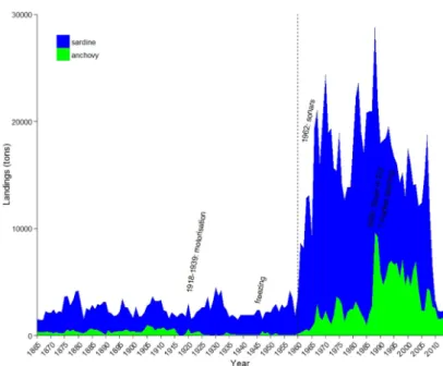
Historically, both species are mainly exploited by the French and the Spanish (Fig. 2). The landings of anchovy have dropped in the early 2000s, probably because of low recruitments (Fig. 1a) and a fragile spawning biomass due to a high fishing pressure (Bueno-Pardo et al., 2020). This decrease led to a four year moratorium from July 2005 until 2010. Since then, the captures have increased thanks to good recruitments and the French landings of anchovy and sardine represented respectively, 3 004 tonnes and 17 218 tonnes in 2018 (mainly driven by the Bay of Biscay). These high landings resulted in sardine being the first landed species in France in 2018 (FranceAgriMer, 2019).
Introduction
Figure 2 – Landings of anchovy and sardine in the bay of Biscay (ICES VIII a, b, c) from 1925 to 2018 (ICES, 2014, 2019c, 2020)
1.2
A general decrease in size and body condition
Over the past two decades, anchovy and sardine have shown an average decrease in size and body condition in the North East Atlantic (Brosset et al., 2017; Doray et al., 2018; Saraux et al., 2019).
This phenomenon has already impacted the fishery, as it is the reason for the decline of small pelagics landings in the Gulf of Lion (north western Mediterranean). In this area, the decrease in size and body condition of anchovy and sardine made them economically unfavorable as there was no market for small individuals. As a consequence, landings have dropped. In the Gulf of Lion, anchovy and sardine used to represent over 50% of annual landings until the 2000s, but sardine has now reached its lowest recorded levels in 150 years (Fig. 3, see Van Beveren et al., 2014, 2016b; Saraux et al., 2019).
The abundance levels of both species remain high (Saraux et al., 2019) whereas the bigger individuals at age and the older individuals disappear (Van Beveren et al., 2014; Brosset et al., 2015; Saraux et al., 2019). In this area, recent studies seem to dismiss a top-down effect (fishing and natural predation) or potential diseases and parasites, in order to explain this decrease in size and condition, but rather explore the lead of a bottom-up control (Brosset et al., 2016a; Van Beveren et al., 2016a; Saraux et al., 2019).
This decrease in size and body condition has also been observed for anchovy and sardine in the Bay of Biscay over the past 20 years (Doray et al., 2018; Véron et al., 2020). This phenomenon has not yet impacted the landings in this area as it did in the Gulf of Lion. However the fishermen, mainly purse seiners, do encounter difficulties in selling small anchovies. Because of their size, canners do no longer sell sardine fillets coming from the Bay of Biscay, as they still used to do few years ago.
In the English Channel, the landings of both anchovy and sardine have never been particularly high. However, their abundance has increased in the North Sea since the mid-1990s (Alheit et al., 2012; Petitgas et al., 2012). For anchovy, this stock has recently proven to be the same as the one of the English Channel (Huret et al., 2020).
Introduction
Figure 3 – Landings of anchovy and sardine in the Gulf of Lion (After Saraux et al., 2019)
1.3
Small pelagic fish growth in relation to the environment
Differences in small pelagics growth can be explained by differences in local environ-ments. This relation between growth and habitat follows a latitudinal gradient. Cold ecosystems are generally associated with bigger individuals having a slower growth rate than the ones living in warm ecosystems. Indeed, in most ecosystems two general rules can be observed : bigger is better and hotter is smaller (Kingsolver and Huey, 2008). The first rule states that bigger individuals are associated to a greater fitness within the same population (Bonner, 2006). Even if being bigger has a cost, as these individuals will increase their demand in energy, it is often worth it, as the bigger is better theory predicts that a directional selection will tend to increase size in most natural populations (Kingsolver and Huey, 2008).
However, the second theory, hotter is smaller, states that for most ectotherms, smaller individuals will be selected in hotter ecosystems (Atkinson and Sibly, 1997; Angilletta and Dunham, 2003).
A latitudinal gradient in size, weight and body condition can be observed for anchovy and sardine in the North East Atlantic, with individuals getting bigger towards high latitudes (Silva et al., 2008; Huret et al., 2019). This gradient is the result of a trade-off between energy demand associated to the size of the organism and the environment. Regardless of the environment, large body size organisms are related to a high reserve quantity and high maintenance costs. They profit from high latitudes ecosystems as those are more productive and require lower maintenance costs, because of lower temperatures. This allows organisms to have enough reserve quantity to survive tougher winters. Indeed organisms living in warmer ecosystems will be smaller because of food limitation and will be constrained by high maintenance costs because of the high temperatures.
If the precise reasons remain unclear, a bottom-up control is so far privileged to explain the decrease in size and body condition over the past twenty years. Through statistical approaches, recent studies highlighted the prominent role of temperature, phytoplankton
Introduction
and zooplankton (Brosset et al., 2016a; Véron et al., 2020). In this way, a modelling framework may help in order to understand which processes are involved in this decrease in size over the last decades.
1.4
Objective of this study
Figure 4 – Map of the studied areas (blue : English Channel, orange : Bay of Biscay, red : Gulf of Lion)
To understand the decrease in size and body condition of small pelagic fish, this study adopts a comparative approach to explore life history traits variability across different areas and different species. The aim being to obtain contrasted environ-ments and to compare the life cycle of two small pelagics in order to improve the robustness of our results. This work is a follow-up to the study of Huret et al. (2019) and is based on the model devel-opped by Gatti et al. (2017). It focuses on the adult stage of two species between 2000 and 2019, anchovy and sardine, both in-habiting three areas : the English Channel (48°N-51°N, 5°W-4.5°E), the Bay of Bis-cay (43°N-48°N, 5°W-0°W) and the Gulf of Lion (42.3°N-52°N, 2.5°E-5.4°E) (Fig. 4). These three regions correspond to three ge-netically different populations for anchovy (Huret et al., 2020) and are all considered as different stocks in terms of management. We will only focus on the effect of the environment on life history traits variability and especially on growth and body condition. Other possible pressures will not be explored (fishing, natural predation, pollution, parasites...) but proposed in the discussion as al-ternative causes.
A first part of this study is about understanding the spatio-temporal variability of the environment to anticipate its capacity in explaining the observed variability in the life history traits. The spatio-temporal variability in length and weight will also be explored as an update of previous studies and in order to standardise the data across the three ar-eas. As anchovy and sardine feed on zooplankton, the use of a model was needed in order to obtain data covering the entirety of each area. We chose to use one single model that covers the three studied areas in order to limit any regional bias. POLCOMS-ERSEM is a coupled physical-biogeochemical model, that provides a synoptic view of the studied areas on a daily basis and detailed information on the lower trophic levels of the marine food web, namely phytoplankton and zooplankton.
Secondly, temperature and zooplankton have been used as forcing variables in a bioen-ergetic model. By quantifying energy fluxes within an organism, bioenbioen-ergetic models enable to understand the impact of a specific environment on the individual’s key func-tions (maintenance, growth, reproduction) at every life stage. In this work we used the Dynamic Energy Budget theory (DEB, Kooijman (2010)) and each species is associated with a DEB model which has been previously calibrated in the Bay of Biscay. These two
Introduction
models are then applied in the three studied areas and over different periods, e.g. early 2000s and mid 2010s. DEB framework also allowed us to investigate energy allocation in comparison to energy density observations which enables to be more accurate than standard morphometric parameters. Our DEB model simulates the average response of a single individual, i.e. individual variability within each region is not investigated.
At last, these models have also been used to explore different scenarios regarding forcing variables (zooplankton and temperature). In order to understand the reason for the de-crease in size of anchovy and sardine, two scenarios were tested. They aimed at further exploring the impact of the temporal variability of the environment and improving the spatialization of the life cycle within each area, in order to fit to the migration patterns. This study aims to better understand the reasons for the decrease in size and body condition of anchovy and sardine, using a comparative approach across areas and species. This approach enables to build a comprehensive modelling framework in order to better understand the processes involved. This work focuses on how does the environment play a role in the variability of life history traits and if a bioenergetic model is able to transcribe this variability.
Material and method
2
Material and method
2.1
Dynamic Energy Budget
2.1.1 Dynamic Energy Budget theory
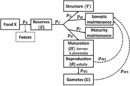
Bioenergetic models simulate the energy flows within living systems. The model used in this study is based on the Dynamic Energy Budget theory (DEB) and applied to individuals. This theory describes the energy assimilation and its allocation to the main biological functions, namely growth, reproduction and maintenance. These energy fluxes depend on the environment (mostly food and temperature) and the state of the organism (Kooijman, 2010; Jusup et al., 2011).
A DEB model is established by defining conceptual compartments (state variables), energy flows between those compartments (energy fluxes) and a set of fixed values (pa-rameters) which are often species specific and enables to adapt the DEB theory to a wide range of organisms.
Figure 5 – Schematic version of the DEB model used in this study (From Gatti et al., 2017)
Variables
State variables (Tab. 1) are defining the system and need to be computed in order to understand the system’s dynamic. There are four state variables : E - the amount of energy in reserve, V - the volume of structural mass, R - the reproduction buffer and H - the level of maturity (Tab. 1).
Assimilated food goes to reserve (E), which is directly linked to food availability. Reserve do not need any maintenance and will be used as a reserve of energy in order to supply the other metabolic processes. The energy is then allocated either to structure (V ), or to reproduction (R). Unlike reserve, structure and reproduction need energy to maintain the tissues that have already been built.
The energy allocation within the organism is based on the κ-rule. A fixed fraction κ is allocated to somatic maintenance and growth, whereas the remaining fraction (1 - κ)
Material and method
Table 1 – State variables of the DEB model
State variables/buffers Formula
Reserve dE dt = ˙pA− ˙pC Volumetric length dL dt = ˙ pG 3[EG]L2 Maturity level dH dt = ˙pR Reproduction dR dt = ˙pR− ˙pR2− ˙pM 2
Gametes if G >= 2Ebatch,dGdt =pGam˙ − ˙pM 3− Ebatch
if G < 2Ebatch,dGdt =pGam˙ − ˙pM 3
is allocated to maturity maintenance and maturation (juvenile) or reproduction (adult) (Fig. 5, see Meer, 2006; Kooijman, 2010; Jusup et al., 2011).
The DEB model used in this study has been developed by Gatti et al. (2017) and has a few characteristics in relation to the classical DEB model that will be mentioned below. Energy fluxes
Different energy fluxes are defined in order to allocate energy among state variables (Tab. 2). As defined by the κ-rule, the main fluxes can be summarised as :
˙
pC = κ ˙pC + (1 − κ) ˙pC = ˙pM + ˙pG+ ˙pj+ ˙pR
Table 2 – Energy fluxes of the DEB model
Fluxes Formula Assimilation p˙A=pAm˙ f L2corL Catabolic utilisation p˙C = (LE3) ˙ ν[EG]L2+ ˙p M [EG]+κE L3 Somatic maintenance p˙M = [ ˙pM]L3 Growth p˙G= max (κ ˙pC − ˙pM, 0) Maturity maintenance p˙j = ˙kjH Reproduction/development p˙R= (1 − κ) ˙pC − ˙pJ
Reproduction buffer mobilisation pR2˙ = min(Ebatch, R)
Gamete allocation pGam˙ = max (0, KR( ˙pR2− ˙pM 2))
Energy maintenance pM 2˙ = min(− ˙pG, R)
Atresia pM 3˙ = min(KRG , − ˙pGam − ˙pM2)
Maintenance always has priority over the other functions, i.e. the organism will stop growing if there is not enough energy available for somatic maintenance. Similarly, ma-turity maintenance has priority over maturation or reproduction. If the maintenance can not be covered by the energy supply of the organism, it dies.
The DEB model used in this study (Gatti et al., 2017) also enables to mobilize energy
from reproduction or gametes ( ˙pM 2, ˙pM 3) if it is needed, in order to ensure somatic
main-tenance and thus, the survival of the organism. This characteristic can be associated to the atresia process.
Material and method
DEB parameters
The parameters are established either based on the literature or by calibration of the DEB model (Tab . 3). By definition, those parameters are fixed values, and most of the time species specific. This set of parameters can be compared to a gene pool. In this way, using the same set of parameters for two distinct populations is almost equivalent to the assumption that these populations are genetically alike and no genetic drift, or any kind of selection that could genetically distinguish these populations, is considered.
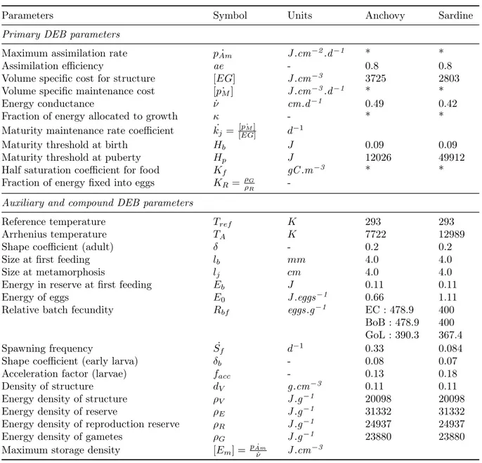
Table 3 – Parameters of the DEB model ; * if optimised in this study, see Tab. 8 ; EC stands for English Channel, BoB for Bay of Biscay and GoL for Gulf of Lion (Adapted from Gatti et al., 2017)
Parameters Symbol Units Anchovy Sardine Primary DEB parameters
Maximum assimilation rate pAm˙ J .cm−2.d−1 * * Assimilation efficiency ae - 0.8 0.8 Volume specific cost for structure [EG] J .cm−3 3725 2803 Volume specific maintenance cost [ ˙pM] J .cm−3.d−1 * *
Energy conductance ν˙ cm.d−1 0.49 0.42 Fraction of energy allocated to growth κ - * * Maturity maintenance rate coefficient k˙j =
[ ˙pM]
[EG] d
−1
Maturity threshold at birth Hb J 0.09 0.09
Maturity threshold at puberty Hp J 12026 49912
Half saturation coefficient for food Kf gC .m−3 * *
Fraction of energy fixed into eggs KR= ρGρR
-Auxiliary and compound DEB parameters
Reference temperature Tref K 293 293
Arrhenius temperature TA K 7722 12989
Shape coefficient (adult) δ - 0.2 0.2 Size at first feeding lb mm 4.0 4.0
Size at metamorphosis lj cm 4.0 4.0
Energy in reserve at first feeding Eb J 0.11 0.11
Energy of eggs E0 J .eggs−1 0.66 1.11
Relative batch fecundity Rbf eggs.g−1 EC : 478.9 400
BoB : 478.9 400 GoL : 390.3 367.4 Spawning frequency S˙f d−1 0.33 0.084
Shape coefficient (early larva) δb - 0.08 0.07
Acceleration factor (larvae) facc - 0.13 0.18
Density of structure dV g.cm−3 0.11 0.11
Energy density of structure ρV J .g−1 20098 20098
Energy density of reserve ρE J .g−1 31332 31332
Energy density of reproduction reserve ρR J .g−1 24937 24937
Energy density of gametes ρG J .g−1 23880 23880
Material and method
2.1.2 Adjustments for small pelagics
Feeding strategy
Anchovy and sardine both feed on diverse plankton organisms with a dominance of copepods (Bachiller and Irigoien, 2015). They also both show an allometric relationship with their prey size range, as the size of fish’s mouth determines the range of available prey. In this way, anchovy and sardine increase their prey size spectrum while growing as they do not avoid small size prey (Bachiller and Irigoien, 2013).
Here, both species are considered to feed exclusively on zooplankton but without any preference in size range.
The amount of available food in the environment (X, food density) in this study, is directly the gross quantity of zooplankton available in the environment which is provided as forcing variable. The scaled functional response is then computed and corresponds to the intake rate of the predator as a function of food density. It is constructed as a Holling
type II function : f = X
X+Kf where Kf is the half saturation rate coefficient.
Spawning strategies
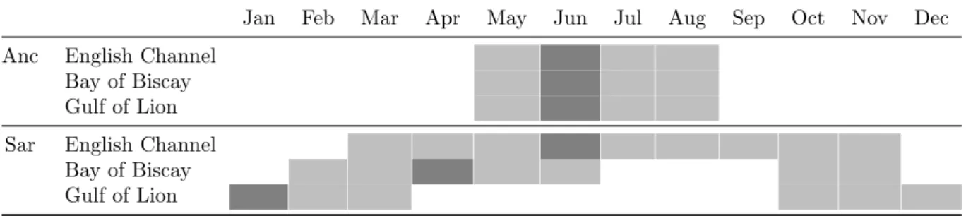
The spawning season changes according to the area and the specie (Tab. 4). For anchovy, the spawning season is the same regardless of the area (Motos et al., 1996; Brosset et al., 2016b; Gatti et al., 2017; Huret et al., 2019). However sardine spawns in spring and summer in the English Channel (Stratoudakis et al., 2007), in winter in the Gulf of Lion (Brosset et al., 2016b) and has two spawning seasons in the Bay of Biscay, in spring and autumn (Gatti et al., 2017). Tab 4 shows the spawning peak in dark grey which also corresponds to the date of birth we set in our DEB model.
Table 4 – Description of the spawning seasons used in this study, dark grey : spawning peak also considered as the date of birth in our model, anc : anchovy, sar : sardine
Jan Feb Mar Apr May Jun Jul Aug Sep Oct Nov Dec Anc English Channel
Bay of Biscay Gulf of Lion Sar English Channel
Bay of Biscay Gulf of Lion
Only one parameter differs among the three studied areas, the relative batch fecundity
(Rbf), which corresponds to the number of eggs per gram (wet mass) of female, released
at each spawning event (batch). For anchovy Rbf is set to 478.9 eggs.g−1 in the English
Channel and the Bay of Biscay, while it is set at 390.3 eggs.g−1 in the Gulf of Lion. For
sardine, Rbf is set to 400 eggs.g−1 in the English Channel and the Bay of Biscay, and to
Material and method
2.2
Fish data
This study focuses on the adult stage, but data about the whole life cycle is needed for the calibration of the DEB model.
2.2.1 Larvae and juveniles
Length (cm) and wet weight (g) data for larvae and juveniles were collected over several years in spring/summer and in autumn in the Bay of Biscay (Tab. 5). These data originate from dedicated surveys and also from a partnership with professionals.
Larvae were caught by using a ’Carré net, an ichtyoplankton net and juveniles were caught by using pelagic trawls. Details can be found in Gatti et al. (2017).
Table 5 – Synthesis of fish data, all of them collected during Ifremer scientific surveys, unless stated otherwise (Anc states for anchovy and Sar for sardine)
Area Source Time series Month coverage Variables Species Larvae Bay of Biscay PLAGIA 1999 Jun-Jul Length, weight Anc
Bay of Biscay MICRODYN 2004 Jun Length, weight Anc Bay of Biscay ECLAIR 2008 Jun-Aug Length, weight Anc Bay of Biscay SENTINELLE 2010 Jul Length, weight Anc, Sar Bay of Biscay PELGAS 2009;2011 May Length, weight Anc Bay of Biscay PELGAS 2009-2013 May Length, weight Sar Juveniles Bay of Biscay JUVESU 1999 Sep Length, weight Anc Bay of Biscay JUVAGA 2003 Oct Length, weight Anc Bay of Biscay Pro Juva 2005 Sep Length, weight Anc
Bay of Biscay JUVENA 2014 Sep Length, weight Anc Adults English Channel PELTICb 2014-2019 Oct Length, weight Anc, Sar
English Channel CAMANOC 2014 Sep-Oct Energy density Anc, Sar English Channel CGFS 2015 Oct Energy density Anc, Sar English Channel Commercial landings 2015-2016 Mar;May;Jul:Nov Energy density Sar
Bay of Biscay PELGAS 2000-2019 May Length, weight Anc, Sar Bay of Biscay PELGAS 2014-2015 May Energy density Anc, Sar Bay of Biscay EVHOE 2014-2015 Oct Energy density Anc, Sar Bay of Biscay Commercial landings 2014-2015 Fev:Nov Energy density Anc, Sar Gulf of Lion PELMED 2002-2019 Jul Length, weight Anc, Sar
aProfessional partnership bCEFAS survey
2.2.2 Adults
Length and weight
The length and weight data for adult stage, are exclusively coming from the dedicated annual pelagic surveys in each of the three studied areas, PELTIC for the English Channel, PELGAS for the Bay of Biscay and PELMED for the Gulf of Lion (Tab. 5). These data have been standardised in order to avoid bias across time or space and are mean values per age, per year and per area. The standard calculation methodology is based on the combination of abundance-at-lengths derived from acoustic data and length-age and length-weight keys. It provides mean lengths and weights-at-age weighted by fish abundance-at-length (using v1.3.9 EchoR package in R, see Doray, 2013).
Material and method
Energy density
Energy density (kJ g−1) is the amount of energy per unit of mass and it has been measured
by following the methods of Dubreuil and Petitgas (2009) and Spitz and Jouma’a (2013). The whole fish is dried and then grinded in order to obtain an homogenize powder. Subsamples are collected and then placed in an adiabatic bomb calorimeter in order to measure the energy released through the combustion.
2.2.3 Exploration of the observed spatio-temporal variability
In order to quantify the decrease in length and weight at age over the past twenty years, linear models have been used considering age, year and area. These models have been applied on adult stage but only for the Bay of Biscay and the Gulf of Lion because of the lack of long time-series in the English Channel.
2.3
Environmental forcing variables
2.3.1 POLCOMS-ERSEM
Environmental variables (temperature and zooplankton) are used as input for the DEB model. Coupled physical-biogeochemical model represent the only source of syn-optic environmental information over space (3D) and time, which in addition incorpo-rates zooplankon component. In this study, we used the regional physical-biogeochemical model POLCOMS-ERSEM (Allen et al., 2001; Holt et al., 2004). This dataset covers the Northwest European Shelf and Mediterranean Sea and is coming from the coupling of a regional ocean circulation model, POLCOMS (Proudman Oceanographic Laboratory Coastal Ocean Modelling System) and a marine ecosystem model, ERSEM (European Re-gional Seas Ecosystem Model). Thus, POLCOMS simulates the hydrodynamics in three dimensions, and ERSEM models the cycles of carbon and major nutrient elements within the lower trophic levels of the marine ecosystem with several groups of phytoplankton and zooplankton (Marsh, 2019).
Using a single model over the three areas should minimise any regional bias due to different modelling assumptions or structure.
2.3.2 Data extraction
Our study uses a configuration in zero dimension (0D), only time is varying and no migration or spatial patterns are considered. It aims to understand the average individual response to an average environment in each of the three studied areas. No spatialization has been made within each area and the averaged value per cubic metre and per day, over the whole area, has been computed. In this way, an average signal is extracted in the form of time series between 2000 and 2015.
To fit to the life cycle of anchovy and sardine, the forcing variables are averaged over 0-30m (eggs, larvae and juvniles) and 0-150m (adults) for temperature and 0-50m for zooplankton.
POLCOMS-ERSEM is structured in cells of 0.1 degree horizontally and 40 σ layers vertically. This implies that the thickness of each layer is dependent on the bathymetry and then not constant across cells. Furthermore, the surface varies among cells when changing units from degree to meter. As the cell’s volume is not constant, a surface and
Material and method
cells’ thickness weighting has been done during the extraction, in order to standardise the data.
The phytoplankton variable has been computed by summing four variables (picophyto-plankton, nanophyto(picophyto-plankton, microphytoplankton and diatoms) and the zooplankton variable has been computed by summing two variables (microzooplankton and mesozoo-plankton).
In this study, the DEB model’s input are daily climatologies, i.e. pluriannual daily means. We chose not to use a succession of years, but rather the averaged year observed during a given period which is then repeated during the whole life cycle of the individual. In this way, we avoid modelling only one single cohort, but rather simulate the average response of an organism to the environment of a given period.
2.3.3 Comparison of POLCOMS-ERSEM with satellite data
To assess the validity of POLCOMS-ERSEM, in particular its capacity to simulate the seasonal and inter-annual variability and trends, we compared its surface tempera-ture and phytoplankton (Chl-a) outputs with satellite data. Those satellite data have been extracted over the same areas and period, and then compared to the surface vari-ables from POLCOMS-ERSEM (first three meters).
The satellite data are available on Copernicus Marine Service (CMS, see marine.copernicus.eu). The sea surface temperature came from the advanced very high resolution radiometer (AVHRR) sensors provided by the AVHRR/Pathfinder (Saulquin and Gohin, 2010), and the chlorophyll-a came from multi-sensor daily analyses (Saulquin et al., 2019). Both variables have been extracted and interpolated by local experts, using kriging method.
2.3.4 Spatio-temporal variability of the environmental variables
Corrections for the Gulf of Lion
The daily resolution data was not available for the whole area of the Gulf of Lion. The Cubic Spline Interpolation (using v1.3.7 RMAWGEN package in R) has been used in order to make the interpolation from monthly to daily data in this area. The Cubic Spline Interpolation uses a string of third order polynomials in order to obtain a smooth function which passes through each data point and avoids continuity breaks or erratic behaviour.
Another issue has been encountered for this area. After discussion with local experts, the seasonality of the zooplankton coming from POLCOMS-ERSEM was not matching the observed seasonality of zooplankton in the Gulf of Lion. To correct this issue, the seasonal effect of the zooplankton was replaced by the seasonal effect of the phytoplankton with one month lag. This has been done by decomposing the original time series in three additive components (trend, seasonal and noise). After checking if the seasonal pattern of phytoplankton from POLCOMS-ERSEM was matching the seasonal pattern observed in the phytoplankton from satellite data, it has been used to correct the seasonality of zooplankton.
Material and method
Environmental data mining
So as to understand the variability in the outputs of the DEB model, a large part of this study focused on understanding the spatio-temporal variability in the inputs of the DEB model, namely the environment variables. To do so, variability and trends from POLCOMS-ERSEM variables have been explored using linear models.
Identification of significantly different periods
One of the aims of this study is to understand if the DEB model is able to explain the decrease in size and body condition that happened over the past twenty years. There is a need to figure out if the environmental variables we are using, show significant differences between the early 2000s and the mid 2010s. A Multiple Factor Analysis (MFA) has been run, followed by a clustering to identify years with similar environments.
2.4
DEB calibration
For each species, one set of parameters has been established by Gatti et al. (2017), either based on literature or estimated by calibration. The calibration has been done for the Bay of Biscay, using the whole fish data set they had (1999-2014), and with environmental forcing coming from a hindcast of ECOMARS 3D (Huret et al., 2013) and averaged over 1980-2008.
This set of parameters has proven to be robust when tested with different data sources (Huret et al., 2019). However, in order to test if the DEB model was able to predict the decrease in size and condition over time, this calibration was problematic. Thus, the choice has been made to make a new parameter estimation based only on the last years of the studied period, as the energy density data are only available for 2014 and 2015 and allow to have a more complete dataset. The forcing variables from POLCOMS-ERSEM were averaged over 2010-2015 and the adults fish data were selected over the 2010-2015 period. However the dataset related to larvae and juveniles was not exhaustive enough to cover the years after 2010. In this way all the available data have been used for the calibration of the young stages.
We tried to modify the minimum number of parameters to rely as much as possible on the work and calibration of Gatti et al. (2017). As such, only the parameters affecting
size and food assimilation have been re-estimated ( ˙pAm, [ ˙pM], κ, Kf).
We used the downhill simplex optimisation (Nelder and Mead, 1965) which is relevant as only four parameters are estimated (using amoeba in Fortran). This few number of parameters should prevent us from finding different optima depending on initial parame-ters. However different set of those initial parameters have been tested in order to avoid local minima.
This Simplex method aims at minimising the following cost function :
F
cost=
stages P i variables P j 1 nobsi,j nobsi,j P kxi,j,k−yi,j
σobsi,j !2
with nobsi,j the number of observations for variable j at life stage i, x the observations,
y the predictions and σobsi,j the observed standard deviation of variable j at life stage i.
Four variables are considered : length, weight, energy density and the number of batches, at three different life stages : larvae, juveniles and adults (according to data availability).
Material and method
2.5
Environmental based scenarios
2.5.1 Improving temporal trends
To investigate how sensitive our model is to the forcing variables, two scenarios (SC) have been explored.
The temporal trends of POLCOMS-ERSEM turned out to be barely significant over 2000-2015 (see Results section). We needed to improve those trends to better explore the hypothesis of a change in the environment supporting the decrease in size of small pelagics. In SC1 we focused on the temporal trend of zooplankton as the trend of temperature was satisfactory enough.
In the same way that we corrected the seasonality of zooplankton in the Gulf of Lion, we decomposed the forcing variables of the DEB model (food and temperature) in three additive components (trend, seasonal and noise). The same decomposition has been ap-plied to the phytoplankton coming from the satellite data.
The trends of the zooplankton has then been replaced by the phytoplankton trend, ob-served in the satellite variable.
2.5.2 Improving spatialization for anchovy
The standard DEB model we used do not account for any spatialization during the life cycle of the individuals or any migration pattern. Though, anchovy do migrates through its life cycle, especially for spawning.
(a) Autumn-winter (b) Spring-summer
Figure 6 – Map of the spatialization of the life cycle of anchovy, between its spawning season (spring-summer) and outside its spawning season (autumn-winter), in the English Channel/North Sea (blue) and in the Bay of Biscay (orange)
Material and method
SC2 is a spatial based scenario and accounts for the migration of anchovy in the En-glish Channel and in the Bay of Biscay as described in Huret et al. (2020). As the exact month corresponding to the start of the migration is not well known, this scenario assumes that migration patterns match the spawning season (Fig 6, Tab. 6).
Outside the spawning season, anchovy is located in the English Channel and on the conti-nental shelf of the Bay of Biscay (Fig. 6a). During its spawning season (spring-summer), anchovy migrates toward the south-east of the North Sea for the English Channel popu-lation and aggregates in the south of the continental shelf in the Bay of Biscay and (Fig. 6b).
Table 6 – Location of anchovy during its migration, according to its spawning season, in dark grey
Jan Feb Mar Apr May Jun Jul Aug Sep Oct Nov Dec English Channel
North Sea Bay of Biscay Bay of Biscay South
As the calibration has been run over the whole Bay of Biscay, this area is not expected to show a particular improvement with the spatialization, but it might highlight variability in our results. However, significant differences are expected in the northern area.
Results
3
Results
3.1
Decrease in length and weight at adult stage
Survey data show a significant decrease in size over the past two decades in the Bay of Biscay and in the Gulf of Lion (Fig. 7). The present lengths and weights in the Bay of Biscay are similar to the lengths and weights observed in the Gulf of Lion in the early 2000s. The time series being relatively short in the English Channel (2014-2019), it is not yet possible to determine if the same pattern is observed in this area.
The decrease is relatively smooth between the early 2000s and the late 2010s, except for sardine in the Gulf of Lion (Fig. 7) where a sharp decline is observed from 2007 to 2011, especially for age 1.
Between the beginning and the end of the time series, anchovy has lost over 10% of its length and over 30% of its weight, both in the Bay of Biscay and in the Gulf of Lion. Sardine is estimated to have lost 9% of its length and 20% of its weight in the Bay of Biscay, and respectively, 20% and over 50% in the Gulf of Lion.
Figure 7 – Length at age for anchovy (top panel) and sardine (bottom panel) in the English Channel (left), the Bay of Biscay (middle) and the Gulf of Lion (right). Averaged pelagic survey data over 2014-2019 in the English Channel (PELTIC survey), 2000-2019 in the Bay of Biscay (PELGAS survey) and 2002-2019 in the Gulf of Lion (PELMED survey)
Results
In order to quantify this decrease, linear models have been applied to both species separately. Three factors have been studied : age, year and area. Anchovy is estimated to have lost 0.15 cm and 0.7 g per year both in the Bay of Biscay and in the Gulf of Lion (Fig. 8).
For sardine, the decreasing rates for length and weight were significantly different per area. It is estimated to have lost 0.12 cm and 1.1 g per year in the Bay of Biscay and 0.24 cm and 1.3 g per year in the Gulf of Lion (Fig. 8).
Figure 8 – Linear model applied to the evolution of length for anchovy and sardine, in the Bay of Biscay and in the Gulf of Lion
3.2
Environment characteristics
3.2.1 Comparisons between POLCOMS-ERSEM and satellite data
The seasonality of POLCOMS-ERSEM was fitting well the seasonality of the satellite data (Fig. 9). This is especially true for the sea surface temperature, which is not surprising, as the forcing variables used in POLCOMS-ERSEM assimilate temperature.
Regarding the chlorophyll-a (Fig. 9), POLCOMS-ERSEM tends to overestimates the mean monthly values when compared to the satellite data. In the English Channel, POLCOMS-ERSEM also overestimates the phytoplankton peak occurring in spring. In the Bay of Biscay, the phytoplankton peak occurring in spring seems to be constantly
overestimated in POLCOMS ERSEM (data exceeding 2 mg.m−3).
Comparing inter-annual mean values from POLCOMS-ERSEM and from satellite data has shown a good fit for temperature (Fig. 10a). However, the fit was very poor for chlorophyll-a (Fig. 10b), especially in the English Channel and in the Bay of Biscay.
Results
(a) SST (b) Chlorophyll-a
Figure 9 – Comparison of the monthly means between satellite and POLCOMS-ERSEM, for sea surface temperature and surface chlorophyll-a over 2000-2015
(a) SST (b) Chl-a
Figure 10 – Comparison of the yearly means between satellite and POLCOMS-ERSEM, for sea surface temperature and surface chlorophyll-a over 2000-2015
Comparing the inter-annual trends between POLCOMS-ERSEM and satellite data over 2000-2015, shows either an absence of significant trends in POLCOMS-ERSEM data or even an opposite trend for the chlorophyll-a in the English Channel (Tab. 7), where
POLCOMS-ERSEM shows an increase of 0 .005 mg.m−3 per year whereas the satellite
shows a decrease of 0 .013 mg.m−3 per year.
3.2.2 Low temporal variability in the environment
Firstly we aimed at quantifying temporal trends in POLCOMS-ERSEM variables, from 2000 until 2015. Only a few variables of phytoplankton and zooplankton showed significant trends, whereas temperature was never significant (Tab. 7). The linear trends
suggest an increase of 0 .005 mg.m−3 of total phytoplankton in the English Channel and
an increase of 0 .08 mgC .m−3 of zooplankton both in the English Channel and in the Gulf
Resul
t
s
Table 7 – Linear trends (per year) and mean values of the environment variables over 2000-2015 (* if not significant)
English Channel Bay of Biscay Gulf of Lion
Units Slope Mean value Slope Mean value Slope Mean value
satellite
Chl-a mg.m−3 - 0.013 1.17 * 0.69 - 0.01 0.48
Sea Surface Temperature °C * 13.1 + 0.02 15.8 * 17.2
polcoms-ersem Chl diatom (3m) mg.m−3 + 0.007 0.84 * 0.38 * 0.25 Chl microphytoplankton (3m) mg.m−3 - 0.002 0.64 - 0.002 0.25 * 0.08 Chl nanophytoplankton (3m) mg.m−3 * 0.31 * 0.25 * 0.16 Chl picophytoplankton (3m) mg.m−3 * 0.16 * 0.14 * 0.1 Chl phytoplankton tot (3m) mg.m−3 + 0.005 1.9 * 1.0 * 0.62 Microzooplankton (50m) mgC .m−3 * 12.7 * 7.6 * 6.8 Mesozooplankton (50m) mgC .m−3 + 0.07 27.4 * 10.6 + 0.03 1.7 Zooplankton tot (50m) mgC .m−3 + 0.08 40.1 * 18.2 + 0.08 8.5 Temperature (3m) °C * 13.0 * 16.1 * 16.7 Temperature (30m) °C * 12.9 * 15.5 * 16.1 Temperature (150m) °C * 12.8 * 13.4 * 15.3 Mémoir e de fin d’études -Cl ar a Menu -Septembr e 2020 19
Results
As the temporal variability was very difficult to evidence from POLCOMS-ERSEM, we tried to identify periods with similar environmental conditions. Multiple Factor Analysis (MFA) has been performed, followed by a clustering, in order to gather similar years. It has not been possible to discriminate significantly different periods, i.e. groups of successive years, however the MFA identified 2007 as a particular year both in the Bay of Biscay and in the Gulf of Lion. This year shows low variability, with a low spring bloom and a relatively high minimum of production in winter in comparison to the other years. As it has not been possible to identify significantly different period in the environment, we chose to average the first five and the last five years as input for the DEB model, i.e. 2000-2005 and 2010-2015.
3.2.3 Spatial variability in the environments
A high spatial variability has been highlighted in POLCOMS-ERSEM data (Tab. 7), with mean values of total phytoplankton and zooplankton multiplied by a factor of 2 across areas from the Gulf of Lion up to the English Channel. Moreover, the composition of zooplankton also differs spatially, as a spatial gradient is observed, especially for the mesozooplankton. On average it represents 20% of the total amount of zooplankton in the Gulf of Lion, 58% in the Bay of Biscay and 68% in the English Channel.
This spatial variability is also highlighted in the climatologies, especially regarding the zooplankton density (Fig. 11).
(a) Temperature 0-30m (b) Temperature 0-150m (c) Zooplankton 0-50m
Figure 11 – Daily climatologies averaged over 2000-2015 per region. Blue : English Channel, orange : Bay of Biscay, red : Gulf of Lion
Results
3.3
DEB model
3.3.1 New estimation of parameters
For anchovy, the new estimation of parameters (Tab. 8) improved the fit of the model to the data from the 2010-2015 period. However, no satisfactory set of parameters has been found for sardine. As the new estimation of parameters did not improve the fit for this specie, we kept the values of Gatti et al. (2017).
Table 8 – Estimated parameters of the DEB model, new estimation for anchovy, estimation of Gatti et al. (2017) for sardine
DEB parameters Symbol Units Anchovy Sardine Maximum assimilation rate pAm˙ J cm−2d−1 654.6 987 Volume specific maintenance cost [ ˙pM] J cm−3d−1 130.0.8 103
Fraction of energy allocated to growth κ - 0.70 0.53 Half saturation coefficient for food Kf gC m−3 2.29 2.69
3.3.2 Model fit
Growth
To quantify the fit of the DEB model to the observed data, the Root Mean Square Error (RMSE) has been computed. In order to compare this value among species, areas and variables, the RMSE has been normalised by its mean value.
Normalised Root Mean Square Error :
N RM SE =
1yv u u t n P i ( ˆyi−yi)2 n
Table 9 – NRMSE values to quantify the fit of the DEB model to the observed data on adult stage (* if no data to compare to)
Anchovy Sardine
Area Period Length Weight Length Weight
NRMSE EC 2000-2005 * * * * - 2010-2015 0.07 0.28 0.09 0.24 BoB 2000-2005 0.08 0.31 0.06 0.21 - 2010-2015 0.07 0.20 0.07 0.15 GoL 2000-2005 0.06 0.36 0.23 0.65 - 2010-2015 0.17 0.18 0.54 2.44
The DEB model has first been calibrated in the Bay of Biscay and then applied to the other areas. For anchovy, the model fitted well the corresponding data (Tab. 9) over the calibrated period (2010-2015, see Fig. 12). However, during summer, the anchovy died in the Gulf of Lion, when the food levels are low and the temperature is high. The environment was not different enough between 2000-2005 and 2010-2015 to explain the decrease in size.
Results
(a) Anchovy 2000-2005 (b) Anchovy 2010-2015
(c) Sardine 2000-2005 (d) Sardine 2010-2015
Figure 12 – Growth model for anchovy and sardine with regional climatologies averaged over 2000-2005 and 2010-2015. Length top) and weight (bottom) at age with a focus on larval and juvenile stages (left) and on the whole life cycle (right). Blue : English Channel, orange : Bay of Biscay, red : Gulf of Lion, crosses : individual values at age at larval and juvenile stages, dots : mean value from pelagic surveys. At adult stage January is indicated (Jan), which occurs at different ages for sardine as spawning seasons differ across areas
For sardine, the same pattern is observed as there was no significant differences in the DEB outputs between the early 2000s and the mid 2010s. The DEB underestimated the weight in the early 2000s and overestimated the length and weight in the mid 2010s. In the Gulf of Lion the model always overestimated both length and weight.
For both species, the model predicts better the length than the weight. This result is not surprising, as reserves, and therefore weight, show high variations during the life cycle of the individual. These high variations generates more difficulties to predict the evolution of weight over the life cycle of the individual.
Results
Energy density
The observed seasonality of energy density (Fig. 13) shows an average increase until the end of the productive period (late summer), then decreases in winter and stays low until early spring.
In comparison to anchovy, sardine has wider seasonal variations and seems to have a sharper increase of body condition during summer in the English Channel than in the Bay of Biscay. This late assumption has to be taken cautiously as the data are scarce for winter in the English Channel.
Older sardines, especially from age 4, show a lower body condition through the season. This phenomenon is particularly pronounced in the English Channel and during the peak of body condition in the Bay of Biscay.
It is rather difficult to apply these conclusions to anchovy, as this specie has fewer age groups.
Figure 13 – Observed seasonality at age of energy density (wet weight) for Anchovy and Sardine over 2014-2015 in the English Channel and in the Bay of Biscay
Results
For both species, the model reproduces relatively well the average pattern regarding body condition, with a peak observed during the productive season and a global decrease over the years.
In the observed data, sardine shows more variability through the season than anchovy. However the model do not transcribe these high peaks (Fig. 14). Body condition is sup-posed to be slightly higher in the English Channel, but this phenomenon is not observed in the model’s outputs regarding sardine, but appears for anchovy.
Figure 14 – Model prediction of energy density (dry weight) for anchovy and sardine. Blue : English Channel, orange : Bay of Biscay, red : Gulf of Lion, dots : individual values at age (2014-2015), solid lines : model prediction (simulation over 2010-2015)
3.4
Energy allocation
We compared the allocation of assimilated energy among DEB compartments across areas and species (Fig. 15). A similar pattern is observed for anchovy in the English Channel and in the Bay of Biscay. The fat accumulates rapidly from March to July, with a maximum somatic condition (reserve in Fig. 15) occurring at the end of the productive period, late summer in the Bay of Biscay and autumn in the English Channel. At the same moment, energy starts to accumulate in the reproduction buffer (reproduction and gametes in Fig. 15). While somatic condition decreases, the reproductive condition increases, with a slight decrease in winter and a peak in spring at the beginning of the spawning season.
Results
For sardine, the peak of somatic condition coincides with the end of the productive period (i.e. early summer, late summer and autumn, for the English Channel, the Bay of Biscay and the Gulf of Lion, respectively). It is then followed by the peak of energy accumulated in the reproduction buffer with the beginning of the spawning season.
Figure 15 – Energy allocation of Anchovy and Sardine across the three studied areas and during the calibration period, 2010-2015
Results
3.5
Environmental scenarios
3.5.1 No significant differences while improving temporal trends
Improving the temporal trends for zooplankton (SC1) did not result in any significant differences in the DEB’s output and could not explain the decrease of size that occurred during these past twenty years (Tab. 10). However in the Gulf of Lion, anchovy did survive until age 2 and died once again in July during the low productive period.
Table 10 – NRMSE values to quantify the fit of the DEB model to the observed data on adult stage. * if no data to compare to, SC0 : base-case scenario, SC1 : temporal trend from satellite data, SC2 : improving spatialization
Anchovy Sardine
Area Period Length Weight Length Weight
NRMSE SC0 EC 2000-2005 * * * * - 2010-2015 0.07 0.28 0.09 0.24 BoB 2000-2005 0.08 0.31 0.06 0.21 - 2010-2015 0.07 0.20 0.07 0.15 GoL 2000-2005 0.06 0.36 0.23 0.65 - 2010-2015 0.17 0.18 0.54 2.44 SC1 EC 2000-2005 * * * * BoB 2000-2005 0.09 0.33 0.06 0.23 GoL 2000-2005 0.05 0.35 0.24 0.74 SC2 EC 2000-2005 * * * * EC 2010-2015 0.11 0.32 - -BoB 2000-2005 0.06 0.20 - -- 2010-2015 0.09 0.30 -
-3.5.2 Larger weight variations while improving spatialization for anchovies
For both the English Channel and the Bay of Biscay, SC2 emphasized the weight gain during the spawning season (Fig. 16). For larvae and juveniles, the model had a lower growth rate than the observed data in the Bay of Biscay, which is certainly because juveniles might spent their first winter in the South of the Bay of Biscay, which has not be taken into account in this scenario.
This gain of weight during the spawning season is driven by an increase of energy allocation to the reproduction buffer (Fig. 17). This scenario has not been run for sardine because of a lack of information on their migration pattern, but these results point out the importance of a finer spatial resolution to improve our understanding regarding the impact of the environment on life history traits.
Results
(a) Anchovy 2000-2005 (b) Anchovy 2010-2015
Figure 16 – SC2 Growth model for anchovy with regional climatologies averaged over 2000-2005 and 2010-2015. Length top) and weight (bottom) at age with a focus on larval and juvenile stages (left) and on the whole life cycle (right). Blue : English Channel, orange : Bay of Biscay, crosses : individual values at age at larval and juvenile stages, dots : mean value from pelagic surveys. At adult stage January is indicated (Jan)
Figure 17 – Energy allocation of Anchovy in the English Channel and the Bay of Biscay, following the migration pattern from SC2, during the calibration period, 2010-2015
Discussion
4
Discussion
4.1
DEB modelling allows to explain part of the spatial variability
of traits
4.1.1 A comprehensive modelling framework
In this study, we used a DEB model to investigate the spatio-temporal variability of traits for anchovy and sardine, in relation to their local habitats. In a context of a global decrease of small pelagics size, we focused on growth variability. As this decrease occurred during the past two decades, four parameters accounting for growth, were re-estimated over 2010-2015.
We used ecosystem model predictions from POLCOMS-ERSEM as forcing variables (zoo-plankton and temperature) for the DEB model. It successfully reproduced the spatial variability observed for anchovy and sardine, across the three studied areas, namely the English Channel, the Bay of Biscay and the Gulf of Lion.
The temporal variability of zooplankton and temperature over 2000-2015, was not strong enough to explain the observed decrease in size over the past twenty years.
4.1.2 Growth
At adult stage, the spatial variability of temperature and zooplankton did explain the main differences in growth across the three studied areas, namely the English Channel, the Bay of Biscay and the Gulf of Lion. We did encounter issues in the Gulf of Lion, regarding survival and size overestimation, as the anchovy did not survive after age 2 and the size of sardine was overestimated.
Differences between predictions and observed data show similar variability levels for both species from the English Channel and the Bay of Biscay, with an error of around 1 cm regarding length and 10 g regarding weight estimation.
4.1.3 Energy condition
In the observed data, both species showed a similar pattern regarding body condition. It reaches its maximal values at the end of the productive season, i.e. in late summer and its lowest values in late winter. Moreover, older individuals showed lower body condition than younger ones, especially regarding the peak of condition. This phenomenon was particularly observed for sardine, as this specie shows a greater number of age class than anchovy and as our dataset was more complete.
We did not have any observed data for energy density in the Gulf of Lion, but recent studies (Brosset et al., 2015; Saraux et al., 2019), have found a similar pattern in this area, with maximal values in summer and minimal in winter. As observed in our data, older sardines were more affected than younger one, by the decrease in condition in the Gulf of Lion (Brosset et al., 2015).
Energy expenses differ between anchovy and sardine. Anchovy is considered as an income breeder, which means that it will acquire energy during the spawning period, whereas sardine is a capital breeder, meaning that it will store energy before the spawning season (Ganias et al., 2007; Pethybridge et al., 2014; McBride et al., 2015). As observed in our predictions, sardine shows higher seasonal variability in body condition than anchovy.
Discussion
Sardine alternates between spring-summer, which corresponds to high intakes but low expenses as it is not its spawning season, and winter where the intakes are low but the expenses are high. Anchovy has lower differences in body condition, as it spawns during summer which thus corresponds to a high expenses season, but the intakes are also high regarding food availability.
However, regarding our climatology in the Gulf of Lion, summer corresponds to the lowest levels of zooplankton through the year. In this area, anchovy is closer to the pattern observed for sardine, with a summer corresponding to high expenses but low incomes which might explain why it did not survive in our predictions.
4.2
Why does the environment not transcribe the temporal
vari-ability of traits ?
4.2.1 Lack of temporal variability in the environmental variables
The interannual variations in the environmental data we used, were barely significant and sometimes in opposition with satellite data and literature. This has been the case for the phytoplankton in the English Channel, where POLCOMS-ERSEM predicts an increasing trend between 2000 and 2015, whereas Gohin et al. (2019) observed a decline of Chl-a in the same area over 1998-2017. Trying to improve this lack of temporal trends in POLCOMS-ERSEM, using the trends from satellite data (SC1) did not significantly impact our predictions.
This lack of significant trends or robustness in the environmental data, might be enhanced by the relative shortness (15 years) of the time series.
In addition to these low interannual variations, we encountered issues regarding the zooplankton’s seasonality in the Gulf of Lion, which had to be corrected. The choice of one single model to simulate our forcing variables had been made in order to limit bias across the three studied areas. However it turned out to lack robustness, especially regarding small areas.
Ramirez-Romero et al. (2020) assessed the skills of such coupled physical–biogeochemical models, including POLCOMS-ERSEM, in the North-western Mediterranean. If the rep-resentation of physical processes was appropriate, they pointed out large differences in the biogeochemical variables. POLCOMS-ERSEM has proven to have non-realistic winter mixing in the Gulf of Lion, which implied issues with the timing and the magnitude of the phytoplankton bloom occurring in winter-spring in this area.
Moreover, they advise to use these models cautiously in the Mediterranean, as they might not be robust enough to reproduce the interannual variation of phytoplankton biomass, which then drives the zooplankton biomass (Ramirez-Romero et al., 2020).
This lack of robustness regarding the timing of the production peak in the Gulf of Lion and the interannual variation, confirms our results.
As the use of a single model has shown its limits, it would be interesting to combine the use of large scale models to site-specific ones. This approach would allow to limit bias across the studied areas, while complying with local habitat characteristics.
The DEB model used in this study has already been used with forcing variables coming from different models and has proven to be robust enough while the forcing variables