Volatility transmission between the oil price, the exchange rate and the stock market index

(1)

Volatility transmission between the oil price, the

exchange rate and the stock market index

Mémoire

Mardochée Bopo Mokengoy

Maîtrise en économique

Maître ès arts (M.A)

Québec, Canada

(2)

(3)

iii

Résumé

Ce mémoire analyse la transmission de volatilité entre le prix du pétrole, le taux de change et l’indice boursier au Canada et aux États-Unis de 1999/01/04 à 2014/03/21. En utilisant un modèle MGARCH-BEKK, nos résultats montrent qu’au Canada, il existe une transmission bidirectionnelle de volatilité entre le taux de change $US/$CAD et l’indice boursier TSX, une transmission positive de l’indice boursier au prix du pétrole, ainsi qu’une transmission négative du taux de change au prix du pétrole. Les résultats suggèrent également que ces relations ne sont pas stables dans le temps. Pour les États-Unis, le modèle estimé ne satisfait pas la condition de stationnarité de la covariance pour la période totale et la sous période 1999/01/04 – 2002/10/08. C’est pourquoi nous considérons uniquement les résultats des sous périodes 2002/10/09 – 2008/05/30 et 2008/06/02 – 2014/03/21. Il ressort qu’il existe des transmissions de volatilité, mais que celles-ci ne sont pas stables dans le temps.

(4)

(5)

v

Abstract

This thesis analyzes the transmission of volatility between oil prices, exchange rates and stock market indices in Canada and in the USA for the period 1999/01/04 – 2014/03/21. Using a multivariate GARCH – BEKK model, we find that in Canada, there is a bidirectional transmission of volatility between the exchange rate $US/$CAD and the stock market index TSX, a positive transmission from the stock market index to the oil price and a negative transmission from the exchange rate to the oil price. We find also that these relationships are not stable over time. For the USA, the model estimated does not satisfy the condition of covariance stationarity for the entire sample and the sub sample 1999/01/04 – 2002/10/08. So we consider only results for sub samples 2002/10/09 – 2008/05/30 and 2008/06/02 – 2014/03/21. Results show that there are transmissions of volatility, but here again, these relationships are not stable over time.

(6)

(7)

vii

List of tables

Table 1 Summary of the seven studies reported on the volatility transmission between oil prices and stock

market indices ... 5

Table 2 Summary of the three studies reported on the volatility transmission between oil prices and exchange rates ... 8

Table 3 Summary of the six studies reported on the volatility transmission between oil prices and exchange rates ... 10

Table 4 Descriptive statistics ... 26

Table 5 Correlation matrix ... 28

Table 6 Parameters with their respective interpretations ... 30

Table 7 Results of BEKK MGARCH estimations for Canada and USA ... 31

Table 8 Canada sub sample results ... 34

Table 9 USA sub sample results ... 36

Table 10 ARCH and GARCH estimations results for Canada ... 38

Table 11 AIC and BIC criteria for estimations results for Canada ... 38

Table 12 ARCH and GARCH estimations results for the USA ... 39

(10)

(11)

xi

List of figures

Figure 1 Oil price, Exchange rate $US/$CAD and Stock market index TSX... 27

Figure 2 Oil price, Exchange rate Euro/$US and Stock market index SP500 ... 27

Figure 3 Volatility transmission in Canada ... 32

Figure 4 Volatility transmission in Canada for period 3 ... 35

Figure 5 Volatility transmission in USA for period 2 ... 37

(12)

(13)

xiii

Acknowledgements

I sincerely thank my supervisor Professor Stephen Gordon for the good supervision that I received from him for carrying out this thesis. I also express my gratitude to Professor Benoit Carmichael, my codirector, for his relevant advice and suggestions.

Finally, I would like to thank my family and close friends for their support and encouragement during my studies.

(14)

(15)

1

Introduction

Volatility is a concept that interests economists because it’s a measure of uncertainty. According to Joshua Aizenman and Brian Pinto (2005), volatility and economic crises are linked because they are driven by the same fundamental phenomenon. They consider for example a situation where weak fiscal institutions and inconsistent macroeconomic policies magnify output volatility. It may well be that such circumstances tend to attract short-term, speculative capital inflows, creating a vulnerability to a sudden stop and hence a crisis down the road. In that sense, volatility could evolve into a crisis. They also show that volatility affects economic growth, by declining investment and increasing inequality in income distribution.

In this study, we focus essentially on volatilities of oil prices, exchange rates and stock market indices, because empirical studies show that each of these volatilities influence some macroeconomic variables related to the business cycle.

An increase in oil price uncertainty (or volatility) reduces industrial production, manufacturing, investment and sustainable consumption. It also leads to a lower average growth rate1_{. An increase in}

exchange rate volatility leads to lower exports, trade flows, domestic consumption, foreign direct investment, and higher unemployment2_{. As for stock market index volatility, empirical studies show that}

it leads to a decrease in consumption of durable goods and is one of the first signs of a coming recession.3

Liu et al (2013) show that changes in volatility indices are closely related to important economic and political events. They illustrate it graphically with the evolution of the volatility indices of stock market (VIX), euro/dollar exchange rate (EVZ), gold price (GVZ) and oil price (OVX) during the sample period from 2008 to 2012. Their graphical analysis shows that there are four significant hikes in the OVX during this sample period. Each of those significant hikes corresponds to an important economic or political event. So, this suggests that these volatility indices are effective measures of the market uncertainty. This also explains our focus on the volatility of the oil price, the exchange rate and the stock market index.

1_{Elder et Serletis (2009,2010), Bredin et al. (2010), Rahman et Serletis (2012)}

2_{Verheyen (2012), Belanger et al (1992), Oskooee et Dan Xi (2012), Renani et Mirfatah (2012), Chang (2011).} 3_{Choudhry (2003), Senyuz et al. (2012)}

(16)

2

In this study, we investigate the interdependence between the three volatilities. The research goal is to see if there is significant transmission of volatility between the oil price, the exchange rate and the stock market index in Canada and in the USA. If so, we determine the direction of this transmission by identifying the driving variable i.e. the one whose volatility shock spreads to others. Then we’ll also check whether it’s a stable relationship or that varies over time.

By volatility transmission we mean how uncertainty in one market spreads to another. Intuitively, uncertainty can be transmitted among these three variables in the following way:

- From the oil price to the stock market index: For a country with a large proportion of the industrial sector in the total production, uncertainty in the oil price can lead to uncertainty in the production level of the country. This last one can in turn lead to uncertainty in the results of companies. Hence, there is uncertainty in the stock market index.

- From the exchange rate to the oil price: For an open economy, uncertainty in the exchange rate can be interpreted as uncertainty about the entry of foreign capital. This can lead to uncertainty in the demand for oil of the country (if the economy is an oil importing). Finally, there will be uncertainty in the oil price.

Other transmissions can be explained by mechanisms similar to those presented above.

It is noted in the literature review that studies on this subject investigate these volatilities by using bivariate analysis. This means that they focus on the link between volatilities of the oil price and the exchange rate, or the oil price and the stock market index, or the exchange rate and the stock market index. The empirical study of Liu et al. (2013) analyzed the link between volatilities of these three variables and the gold price. To the best of our knowledge, this is the only study that makes a link between volatilities of our three variables.The other goal of our study is to confirm or invalidate the previous findings in the Canadian and US contexts.

The importance of carrying out this study is that the results may be useful for economic public and private decision makers. Public decision makers can use the results of this study to take proactive measures of economic policy. In case of a significant transmission of volatility, it will be possible to predict the response of the other two variables after a shock on the volatility of the variable considered as a driver. Depending on the expected reaction of these two variables, public decision makers can

(17)

3

anticipate measures needed to be taken in order to respond to those shocks. Private decision makers can use the results of this study to better understand the stock market volatility in order to better manage their investments.

The importance of analyzing all the three volatilities together is that in case of a significant transmission of volatility, it would be interesting for economic agents involved in these three markets to know the spread sequence of this volatility and the intensity in each market. Furthermore, the fact that few empirical papers have focused on this also justifies our interest in a simultaneous analysis of the three markets.

In this study, we’ll use daily data from 1999 to 2014 and we’ll estimate a conditional heteroskedastic multivariate model.

(18)

(19)

5

I. Literature review

In this section, we present empirical studies that have analysed volatility transmission between and among the three variables of our study. As noted in the Introduction, most of studies on this subject investigate these volatilities by using bivariate analysis. So, this section is divided in subsections according to the variables for which the transmission of volatility was studied:

- Oil price and stock market index ; - Oil price and exchange rate ;

- Exchange rate and stock market index ;

- Oil price, exchange rate and stock market index.

I. 1. Oil price and stock market index

Empirical studies here have quite heterogeneous results according to countries or group of countries studied.

Table 1 Summary of the seven studies reported on the volatility transmission between oil prices and stock market indices

Author Data/countries studied Volatility transmission Aloui et al.

(2008)

Daily (Jan 89. to Oct.2007) France, USA, Japan, Germany,

Canada and United kingdom

Unidirectional (The direction of transmission is

not the same for all countries) Malik and

Ewing

(2009) Five sector stock indices of USA Weekly (Janv.92 to April 2008)

Unidirectional (The direction of transmission is

not the same for all sectors) Shaharudin

et al (2009)

Daily (Aout 2003 to Aout 2008) stock price of Oil and Gas companies, (USA, India and UK)

Unidirectional (From oil price to stock market

index) Arouri et al.

(2011)

Weekly (Jan. 1998 to Dec. 2009) European and American sector

stock indices

Unidirectional in Europe (form oil price to stock market

index) and Bidirectional (in USA) Oskooe

(2011) Weekly (Janv. 1999 to Dec. 2010) Iran No transmission Awartani

and Maghyereh

(2012)

Weekly (Jan. 2004 to March 2012) Gulf Cooperation Council

Countries Bidirectional

Chaibi and Gomes

(2013) Weekly (Jan. 1998 à Dec. 2009) Panel of 54 countries

Unidirectional (From oil price to stock market

(20)

6

As shown in Table 1, for the seven empirical studies that we have chosen, results are distributed as follow:

- three empirical studies find unidirectional transmission (but not always in the same direction) ; - Two find unidirectional and bidirectional transmissions ;

- One finds a bidirectional transmission ;

- And in the last one, there is no transmission of volatility.

I.1.1 Unidirectional transmission

Among the four studies that find unidirectional volatility transmission, there is the one by Aloui et al. (2008), which considers the oil price and six major financial markets of the world (France, USA, Germany, Japan, United Kingdom and Canada). The authors use two indicators for the oil price (West Texas Intermediate and Brent). Results show a positive transmission of volatility from the stock market index to the WTI, while for the USA the direction is in reverse sense.

Malik and Ewing (2009) also analyzed the volatility transmission between oil prices and stock market indices. However, the particularity of their study is that they considered five different sector indices of one country (USA): The financial, industrial, consumer, health, and technology sectors.

Using weekly data from 1992 to 2008, they find a transmission of volatility from financial, industrial and consumer sectors to the oil price. The direction of transmission is in reverse for volatilities of healthcare and technology sectors.

Shaharudin et al. (2009) focus their analysis on oil price and stock price of oil and gas companies in USA, India and UK. Using daily data from 2003 to 2008 and a GJR-GARCH model, they find a volatility transmission in each of these countries, going from the oil price to the stock price of those companies.

I.1.2 Unidirectional and bidirectional transmissions

Empirical studies with unidirectional and bidirectional transmissions findings include those by Arouri et al. (2011) and Chaibi and Gomes (2013).

Arouri et al. (2011) perform their analysis by considering the oil price and European and American stock market sector indices (automobile, financial, industrial, technology, basic materials, telecommunications and public services).

(21)

7

Using weekly data from 1998 to 2009 and a VAR-GARCH model, they find a unidirectional volatility transmission, going from the oil price to industrial sector indices in Europe, while in the USA, the transmission is bidirectional. However,the intensity of this transmission varies according to sectors. The authors explain that this is due to factors specific to each sector, such as the level of oil consumption, competition and concentration in the sector.

Chaibi and Gomes (2013) perform their study by focusing on financial markets of emerging market economies (called frontier markets) and developed ones. They use a sample larger than the preceding studies. For these emerging market economies, they consider national index of each country (21 countries) and «MSCI frontier markets», which is «a free float-adjusted market capitalization index that is designed to measure equity market performance of frontier markets».4_{For developed market}

economies, the «MSCI world» was used.

Results show that there is a significant transmission of volatility between the oil price and financial markets. As for the direction, it is more often from the oil price to financial markets than the reverse. A bidirectional transmission was detected in some emerging market economies (Jordan, Oman, Kazakhstan, Kuwait and United Arab Emirates). It should be note that this study uses data from 2008 to 2013, which correspond to a turbulent period in financial markets (with the financial crisis of 2008). The authors believe that some conjunctural factors may have biased the results of some transmissions of volatility, because in time of crisis, contagion or transmission effects are emphasized.

I.1.3 Bidirectional transmission

Awartani and Maghyereh (2013) investigate the dynamic spillover of return and volatility between oil and equities in the Gulf Cooperation Council Countries during the period 2004 to 2012. Their results indicate that there are bidirectional and asymmetric transmissions, and the oil market sends to other markets more than it receives. The authors explain this asymmetry by the fact that an increase in the oil price generates more income and wealth in the oil exporting countries, thereby stimulating economic activity and financial markets. So, considering these variables in levels, the causality runs from the oil price to financial markets. This explains why the transmission is greater from the oil price to the stock market, than the reverse.

(22)

8

I.1.4 No transmission

Oskooe (2011) performs his study for Iran and finds that there is no volatility spillover between these two variables. According to the author, «the lack of volatility spillover between Iran stock market and international oil market implies the sustainable long - term performance of Iran stock market and invulnerability of it to external shocks in particular oil shocks. This can be good sign to foreign investors and internationally portfolio managers».5

We can see that results of studies on the volatility transmission between oil prices and financial markets are quite heterogeneous, since there is not a specific direction related to the characteristics of the country or a given category of countries. As presented above, the results of Aliou et al. (2008), Oskooe (2011) and Chaibi and Gomes (2013) do not have the same direction for volatility transmission, especially concerning oil exporting countries (Canada, Iran and Kuwait). So we see that for countries with a common characteristic in terms of oil exporting, results are quite different. However, we note that in case of unidirectional transmission, the direction is more often from the oil price to the stock market index.

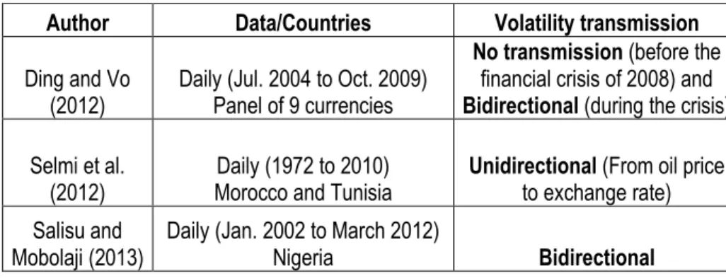
I. 2. Oil prices and exchange rates

We present here three empirical studies that focus on the oil price and the exchange rate. The three studies find different results.

Table 2 Summary of the three studies reported on the volatility transmission between oil prices and exchange rates

Author Data/Countries Volatility transmission Ding and Vo

(2012) Daily (Jul. 2004 to Oct. 2009) Panel of 9 currencies

No transmission (before the financial crisis of 2008) and Bidirectional (during the crisis) Selmi et al.

(2012) Morocco and Tunisia Daily (1972 to 2010) Unidirectional (From oil price to exchange rate) Salisu and

Mobolaji (2013) Daily (Jan. 2002 to March 2012) Nigeria Bidirectional

5_{Oskooe (2011)}

(23)

9

Ding and Vo (2012) perform their study for exchange rates on a panel of 9 currencies, including eight evaluated against the American dollar. The exchange rate used for the American dollar is the US dollar trade weighted index (USX). The eight other currencies are the Canadian dollar (CAD), the Norwegian krone (NOK), the euro (EUR), the Indian rupee (INR), the Japanese yen (JPY), the Singaporean dollar (SGD), the Brazilian real (BZR), the Mexican peso (MXP).

The choice for these currencies is justified as follow:

- The Canadian dollar, The Norwegian krone and The Mexican peso represent exchange rates

of oil exporting countries,

- The euro and the Japanese yen represent developed oil importers,

- The Indian rupee and the Brazilian real represent developing oil consumers,

- The Singapore dollar is used as a neutral currency that is neither a major oil importer nor an exporter.

With daily data from 2004 to 2009 and using a multivariate model, they find results that vary over time. Results show that when the markets are relatively calm (before the 2008 crisis), both oil and foreign exchange markets respond to shocks simultaneously and no interaction is detected. But during turbulent times, there is bidirectional volatility interaction between the two variables.

According to the authors, this bidirectional volatility transmission is consistent with what is seen in the literature, which is that there is a bidirectional causality between the two variables in levels, thus explaining the bidirectional transmission of their volatilities.

The authors attribute the insignificant interaction before the financial crisis to the finding of Chan et al. (2011), whose results indicate that when the markets are relatively calm, both oil and foreign exchange markets respond to information shocks simultaneously, thus failing to exhibit lead-lag behavior in either direction.

Selmi et al. (2012) focus on a small oil importing economy (Morocco) and a small oil exporting country (Tunisia). The particularity of their study is that they consider a given direction of transmission. In fact, the goal of their study is not to determine the direction of the volatility transmission, but rather to determine the impact of the variability of oil price on the real exchange rate, and to compare this impact depending on the nature of the country (oil importing or exporting and exchange rate regime).

(24)

10

Their results reveal that whether for importing or exporting-oil economy, the real price of oil is negatively and significantly related to the variability of real exchange rate. They find also that the effect of bad news is more intense than the good news, i.e. the relationship between oil prices and the exchange rate reacts more to good news than bad news for Morocco, while for Tunisia this effect is contrary. Salisu and Mobolaji (2013) perform their study using Nigerian daily data from 2002 to 2012 and a VAR-GARCH model, they find a bidirectional transmission of volatility between the two variables.

Thus, we see that each of these three studies lead to different results. Here also, there is no specific direction determined by the characteristics of the country or a given category of countries.

I. 3. Exchange rates and stock market indices

Here again, studies find heterogeneous results according to countries.

Table 3 Summary of the six studies reported on the volatility transmission between oil prices and exchange rates

Author Data/Countries Volatility transmission

Kanas (2000)

Daily (Jan. 1986 to Feb. 1998) USA, Royaume Uni, Japon,

Allemagne et Canada

Unidirectional (from stock market index to exchange rate

in USA, UK, Japan and Canada) and No transmission

(in Germany)

Yang and

Doong (2004) Weekly (May 1979 to Jan. 99) G7 countries

Unidirectional (From stock market index to exchange rate,

in France, Italy, Japan and USA) and No transmission (in

Germany, Canada and UK) Mishra et al.

(2007)

Daily (jan.93 to Déc. 2003) India

Bidirectional and Unidirectional (From stock market index to exchange rate) Zhao (2010) Monthly (Jan. 91 to June 2009) China Bidirectional

Chkili et al.

(2012) Daily (Jan. 99 to Dec. 2009) Germany, France and UK Bidirectional Caporale et

al. (2013)

Weekly (Aout 2003 to Dec. 2011) USA, UK, Canada, Japan, Euro

(25)

11

As presented in Table 3, the results of six empirical studies that we consider are distributed as follow: - two find a bidirectional transmission,

- Two others find a unidirectional transmission and a lack of transmission, - The last two find a bidirectional and unidirectional transmissions.

I.3.1 Bidirectional transmission

The two empirical studies that find a bidirectional transmission are those by Zhao (2010) and Chkili et al. (2012).

Zhao (2010) performs his study for China. Using monthly data and a multivariate GARCH model, he finds a bidirectional transmission of volatility between these two variables. According to him, the transmission from the exchange rate to the stock market index can be explained by the fact that the changes of exchange rate influence indirectly the market power of firms’ products in international markets. Since the Chinese economy is export oriented, changes in the exchange rate will influence the quantities of exports. The decrease in the quantities reduces profits of listed firms, therefore the volatility of exchange rate can influence the volatility of the stock price.

For the reverse direction, he explains that the emerging stock market in China attracts foreign investors, so foreign capital may flow into and out of China’s stock markets through underground channels. Chkili et al. (2012) consider three European countries: Germany, France and The United Kingdom. Their results also show that there is a positive bidirectional transmission between the two variables. However, they note that the transmission is more important in Germany and France than in the United Kingdom.

I.3.2 unidirectional transmission and lack of transmission

Kanas (2000) performs his study for the USA, the UK, Japan, Germany and Canada with daily data from 1986 to 1998. He finds a unidirectional transmission in all countries except Germany. This unidirectional transmission is positive and symmetric.

According to the author, the presence of volatility spillovers from stock returns to the exchange rate movements may be interpreted as evidence that the US, UK, Japanese, French and Canadian financial markets are highly integrated. Moreover, he considers that the failure to find a statistically significant

(26)

12

spillover coefficient for Germany may be due to Bundesbank interventions in currency markets during the lifetime of the Exchange Rate Mechanism, which may have affected both the level and the volatility of German exchange rate changes.

Yang and Doong (2004) focus their study on G7 countries. With weekly data from 1979 to 1999, they estimate a multivariate EGARCH and find a unidirectional transmission (from stock market indices to exchange rates) in France, Italy, Japan and USA. In Germany, Canada and the UK, they find no volatility transmission.

Note that the results of this study are consistent with those by Kanas (2000) for Germany and USA, while for UK and Canada, results are not the same. Kanas (2000) finds a unidirectional transmission for these two countries.

I.3.3 Bidirectional and unidirectional transmissions

Mishra et al. (2007) perform their study for India. Using daily data and four stock market indices, they find a bidirectional transmission for two indices and a unidirectional for two other indices.

Caporale et al. (2013) consider a large panel of countries (USA, UK, Canada, Japan, Euro Zone and Switzerland). They use weekly data from 2003 to 2011, which they divide in two sub-periods: a tranquil or pre-crisis period from August 6, 2003 to August 8, 2007, and a crisis period from August 15, 2007 to December 28, 2011.

Their results suggest the existence of causality-in-variance that operates as an information flow, from exchange rate changes to stock returns in the UK, Japan, and Canada in the pre-crisis period. In the crisis period, there is evidence of causality-in-variance from stock returns to exchange rate changes in Japan, in the opposite direction in the euro area and Switzerland, and of bidirectional feedback in the US and Canada.

Thus, we see that the results of studies on volatility transmission between the exchange rate and the stock market index are as heterogeneous as those presented earlier.

We even note that for some countries, the results differ from one study to another. In Canada for example, three different studies (Kanas 2000, Yang and Doong 2004, Caporale et al. 2013) find quite different results. This can be partly explained by the fact that the study period and frequency of data

(27)

13

are not always the same (even though these periods may overlap). So, studies on this subject lead to very heterogeneous results. Note however that in case of unidirectional transmission of volatility, the direction is most often from the stock market index to the exchange rate.

I.4. Oil prices, exchange rates and stock market indices

To the best of our knowledge, the paper of Liu et al. (2013) is the only one that makes a link between volatilities of the oil price, the exchange rate and a stock market index. There are studies that analyze interactions between the three variables (or more) in levels6_{or that make a multivariate GARCH}

modeling, but without checking the volatility transmission among variables.7

Liu et al. (2013) consider gold as well as the three other variables. However, the study has the particularity that volatilities considered for variables are indices OVX (Oil volatility index), VIX (stock market volatility index), EVZ (euro/dollar exchange rate volatility index) and GVZ (Gold price volatility index). These indices represent implied volatilities which are often referred to the market’s perception of future volatility over the remaining life of the option.8_{They are influenced by the price and the maturity}

of the option and the level of the risk-free interest rate. These indices are calculated by CBOE (Chicago Board of Exchange) and are used to predict future market movements. They are described as the «fear indices» because their high levels reflects a high degree of instability to come in the markets.

Using daily data from 2008 to 2012 and a VAR model, Liu et al. (2013) find that there is transmission of volatility between the markets considered. This transmission is positive and unidirectional, going from the financial market, exchange rate and gold price to the oil price.

Among these variables, the one which has the smallest impact on the oil price is the exchange rate. According to the authors, this is mainly because the exchange rate market tends to be more stable than other markets over the whole sample period and the influence of uncertainty shocks in the exchange rate market on commodity markets are relatively weaker compared to the stock market. To investigate the robustness of the results, the authors divide the whole sample period into two sub periods: 2008/6/3 to 2009/6/30 as the crisis outbreak period and 2009/7/1 to 2012/7/20 as the

6_{Basher et al. (2012), Wang and Chueh (2013), Jain and Ghosh (2013), Śmiech and Papież (2013)} 7_{Cifarelli and Paladino (2010)}

8_{Eugenie M.J.H Hol, Empirical studies on volatility in international stock markets, Boston, Kluwer Academic,}

(28)

14

crisis recovery period. The new results indicate that there is no significant «lead-lag» relationship between OVX and the other volatility indices according to the Granger test results in the crisis outbreak period. The post-crisis results are consistent with their main findings, which show that changes in volatility expectation in the crude oil market are significantly caused by others.

The authors explain the change of relationship between the first and the second sub-period by: - The fall of VIX that was mainly due to the quantitative easing (QE) policy and the creation of

extra liquidity by the Federal Reserve. In addition, some «free» money also went into commodities such as oil, which to some extent caused a new boom in these markets. - Shale oil production brought by the shale gas revolution in North America has increased quickly

and has imposed a large downside pressure on crude oil price in North America since the second half of 2010.

This is why the authors consider that these changes in the economic condition and energy markets have brought new challenges to understanding volatility transmission between the oil and other markets. Therefore, they suggest that general conclusions on the relationships among these volatility indices need to be revisited using a longer sample in the future.

So we can learn from this literature review, on the one hand, that the results are heterogeneous, in so far as there is no particular direction emerged in the characteristics of the countries. On the other hand, in case of volatility transmission, there is possibility that this direction varies over time.

(29)

15

II. Methodology

The methodology used to carry out this study is the multivariate GARCH (MGARCH) model. In this section, we present first an introduction to the univariate volatility modeling (ARCH and GARCH models). Next, we present a multivariate version and specify the different variants of that model. Finally, we present and justify the variant of MGARCH model chosen to perform our study.

II. 1. Univariate modeling

Engle’s paper (1982) is considered as the pioneer in volatility modeling. He introduces the ARCH (Autoregressive Conditional Heteroskedasticity) model, a way to model the dynamics of the conditional variance. Bollerslev (1986) introduces a generalization of the ARCH model with the GARCH model (Generalized Autoregressive Conditional Heteroskedasticity), which allows the conditional variance to be an ARMA process and to have a much more flexible lag structure.

The ARCH (q) model proposed by Engle is presented below: 𝑟𝑡 = 𝜇 + 𝜀𝑡

𝜀𝑡 = √ℎ𝑡 𝑍𝑡 𝑍_𝑡

~

𝑁(0,1)

ℎ_𝑡 =𝑤 + ∑𝑞𝑗=1𝑗 𝜀𝑡−𝑗2 

In order to ensure a strictly positive variance, conditions 𝑤 ˃ 0 and _𝑗 ≥ 0 must be respected. If

∑𝑞𝑗=1𝑗 ˂ 1, the ARCH process is weakly stationary with constant unconditional variance :

𝜎2₌ 𝑤 1 − ∑𝑞_𝑗=1𝑗 

The extension of the ARCH (q) model by Bollerslev (1986) to GARCH (p,q), modified the equation of ℎ_𝑡 as follows :

ℎ𝑡 = 𝑤 +∑𝑝𝑖=1𝛽_𝑖ℎ𝑡−𝑖+∑ 𝑗

𝑞

𝑗=1 𝜀𝑡−𝑗2 

The strictly positivity of the variance is ensured here by the conditions 𝑤 ˃ 0, 𝛽_𝑖≥ 0 and _𝑗 ≥ 0, and the stationarity of the process by ∑𝑝_𝑖=1𝛽_𝑖+ ∑𝑞_𝑗=1_𝑗 ˂ 1 .

(30)

16

𝐿_𝑡() = −1₂𝑙𝑜𝑔 ℎ_𝑡− 1₂_𝑡2_ℎ 𝑡 −1

II. 2. Multivariate modeling

Multivariate GARCH (MGARCH) models generalize the univariate GARCH et allow for volatility spillovers in that volatility shocks to one variable might affect the volatility of other related variables.9

Studies with MGARCH allow us to answer questions such as : «Is the volatility of a market leading the volatility of other markets? Is the volatility of an asset transmitted to another asset directly (through its conditional variance) or indirectly (through its conditional covariances)? Does a shock on a market increase the volatility on another market, and by how much? Is the impact the same for negative and positive shocks of the same amplitude?» 10

The general MGARCH model can be written as : 𝑌_𝑡= 𝐶𝑋_𝑡+ 𝜀_𝑡

𝜀𝑡= 𝐻𝑡1/2𝜈𝑡

Where 𝑌𝑡 : is a vector of k dependent variables

𝐶 : is a matrix of parameters

𝑋𝑡 : is a vector of independent variables

𝐻_𝑡1/2 : is the Cholesky root of the time varying conditional covariance matrix H_t (which must be positive definite)

𝜈𝑡 : is a vector of zero mean, unit variance and iid innovations

The various MGARCH models proposed in the literature differ in how they trade off flexibility and parsimony in their specifications for 𝐻𝑡.

Bauwens et al. (2006) distinguish three non mutually exclusive approaches for constructing multivariate GARCH models:

- Direct generalizations of the univariate GARCH model of Bollerslev (1986): There are especially Vector (VEC), Baba Engel Kroner Kraft (BEKK) and factor models.

9_{Walter ENDERS, Applied Econometric time series, New Jersey, Wiley, 2010, p.165.}

10_{Luc Bauwens et al., « Multivariate GARCH models: A survey », Journal of applied econometrics, n}0 ₂₁

(31)

17

- Linear combinations of univariate GARCH models: in this category, there are (generalized) orthogonal models and latent factor models.

- Nonlinear combinations of univariate GARCH models : This last category contains constant and dynamic conditional correlation models (CCC and DCC), the general dynamic covariance model and copula-GARCH models

We’ll present here the following models: Constant Conditional Correlation (CCC), Dynamic conditional correlation (DCC), Vector (VEC) and Baba Engel Kroner Kraft (BEKK). MGARCH CCC and DCC are part of the conditional correlation (CC) models of MGARCH.

II. 2.1. Conditional correlation MGARCH

In conditional correlation (CC) MGARCH models, conditional variances are modeled as univariate GARCH and conditional covariances as nonlinear functions of the conditional variances. In each of the conditional correlation models, the conditional covariance matrix is positive definite by construction and has a simple structure, which facilitates parameter estimation.

In CC models, 𝐻_𝑡 is decomposed into a matrix of conditional correlations 𝑅_𝑡 and a diagonal matrix of conditional variances 𝐷𝑡: 𝐻𝑡 = 𝐷𝑡𝑅𝑡𝐷𝑡 Where : - 𝐷𝑡 = 𝑑𝑖𝑎𝑔(ℎ_11𝑡 1 2 _{. . . ℎ} 𝑁𝑁𝑡 1 2 ₎

- each conditional variance (ℎ𝑖𝑖𝑡) follows a univariate GARCH process

- the parameterization of 𝑅_𝑡 varies across models

II. 2.1.1. Constant Conditional Correlation (CCC) MGARCH

The CCC MGARCH model proposed by Bollerslev (1990) restricts the conditional correlations matrix 𝑅_𝑡 to be constant.

The CCC model is defined as:

𝐻_𝑡 = 𝐷_𝑡𝑅𝐷_𝑡 = (𝜌_𝑖𝑗√ℎ𝑖𝑖𝑡ℎ𝑗𝑗𝑡)

(32)

18

The CCC model in the case of N=3 is:

ℎ_11𝑡 = 𝑎₁₁+ 𝑏₁₁𝜀_1𝑡−12 _{+ 𝑐} 11ℎ11𝑡−12 ℎ22𝑡 = 𝑎22+ 𝑏22𝜀2𝑡−12 + 𝑐11ℎ22𝑡−12 ℎ33𝑡 = 𝑎33+ 𝑏33𝜀3𝑡−12 + 𝑐33ℎ33𝑡−12 ℎ12𝑡 = 𝜌12√ℎ11𝑡ℎ22𝑡 ℎ_13𝑡 = 𝜌₁₃√ℎ11𝑡ℎ33𝑡 ℎ_23𝑡 = 𝜌₂₃√ℎ_22𝑡ℎ_33𝑡

Note that 𝜌_𝑖𝑗 is a time-invariant weight interpreted as a conditional correlation.

II. 2.1.2. Dynamic conditional correlation (DCC) MGARCH

Engel (2002) introduces a DCC MGARCH model, which is an extension of CCC MGARCH, because it allows the conditional correlation (the R matrix) to vary over time.

The model is defined by:

𝐻𝑡 = 𝐷𝑡𝑅𝑡𝐷𝑡 = (𝜌𝑖𝑗𝑡√ℎ𝑖𝑖𝑡ℎ𝑗𝑗𝑡)

𝑅_𝑡 = 𝑑𝑖𝑎𝑔(𝑄_𝑡)−1/2_𝑄

𝑡𝑑𝑖𝑎𝑔(𝑄𝑡)−1/2

𝑄𝑡 = (1 −1−2)𝑄̃ +1𝜀̃𝑡−1𝜀̃𝑡−1′ +2 𝑄𝑡−1

Where: 𝑄𝑡 is a sequence of covariance matrices

𝑄̃ is the N x N unconditional variance matrix of 𝜀̃_𝑡

1 and 2 are non-negative scalar parameters satisfying 1+2 < 1

Considering the non matricial form, we have: 𝜌_𝑖𝑗𝑡 = 𝑞𝑖𝑗𝑡

√𝑞𝑖𝑖𝑡𝑞𝑗𝑗𝑡

𝑞_𝑖𝑗𝑡 = 𝜌̃_𝑖𝑗 +₁(𝜀̃_𝑖𝑡−1𝜀̃_𝑗𝑡−1− 𝜌̃_𝑖𝑗) +₂(𝑞_{𝑖𝑗𝑡−1}− 𝜌̃_𝑖𝑗) Where 𝜌̃_𝑖𝑗 is the unconditional correlation between 𝜀̃_𝑖𝑡 and 𝜀̃_𝑗𝑡.

In the case of N=3, the equations ℎ11𝑡, ℎ22𝑡 and ℎ33𝑡 are the same with those of the CCC model. For

the conditional covariances ℎ12𝑡, ℎ13𝑡 and ℎ23𝑡 the difference with the CCC model is that the

(33)

19 𝜌12𝑡 = 𝑞_12𝑡 √𝑞11𝑡𝑞22𝑡 𝜌_13𝑡 = 𝑞13𝑡 √𝑞11𝑡𝑞33𝑡 𝜌_23𝑡 = 𝑞23𝑡 √𝑞22𝑡𝑞33𝑡 𝑞12𝑡 = 𝜌̃12+1(𝜀̃1𝑡−1𝜀̃2𝑡−1− 𝜌̃12) +2(𝑞12𝑡−1− 𝜌̃12) 𝑞_13𝑡 = 𝜌̃₁₃+1(𝜀̃1𝑡−1𝜀̃3𝑡−1− 𝜌̃13) +2(𝑞13𝑡−1− 𝜌̃13) 𝑞_23𝑡 = 𝜌̃₂₃+₁(𝜀̃_2𝑡−1𝜀̃_3𝑡−1− 𝜌̃₂₃) +₂(𝑞_23𝑡−1− 𝜌̃₂₃)

II. 2.2. Vector (VEC) model

The VEC model was proposed by Bollerslev et al. (1988). In this model, every conditional variance and covariance is a function of all lagged conditional variances and covariances, as well as lagged squared errors and cross products of errors.

For a VEC model (p,q), the model is defined as :

𝑉𝑒𝑐ℎ(𝐻_𝑡) = + ∑𝑞 𝐵_𝑖𝑉𝑒𝑐ℎ(𝜀_𝑡−𝑖𝜀_𝑡−𝑖′ ₎

𝑖=1 + ∑𝑝𝑗=1𝐶𝑗 𝑉𝑒𝑐ℎ(𝐻𝑡−𝑗)

Where :

- 𝑉𝑒𝑐ℎ(. ) is an operator that stacks the columns of the lower triangular part of its argument square matrix

-  is a (𝑁 𝑥 𝑁+1₂ ) 𝑥 1 vector,

- 𝐵_𝑖 and C_iare (𝑁 𝑥 𝑁+1₂ ) 𝑥 (𝑁 𝑥 𝑁+1₂ ) parameter matrices.

In the trivariate case of a VEC model (1,1), 𝐵_𝑖 and 𝐶_𝑖 are all (6 𝑥 6) matrices and equations of the model will be defined as follows :

(34)

20 ( ℎ_11𝑡 ℎ_12𝑡 ℎ_13𝑡 ℎ_22𝑡 ℎ23𝑡 ℎ33𝑡) = ( 𝑎11 𝑎12 𝑎₁₃ 𝑎₂₂ 𝑎₂₃ 𝑎₃₃) + ( 𝑏₁₁ 𝑏₁₂ 𝑏₁₃ 𝑏₂₁ 𝑏₂₂ 𝑏₂₃ 𝑏₃₁ 𝑏₃₂ 𝑏₃₃ 𝑏₁₄ 𝑏₁₅ 𝑏₁₆ 𝑏₂₄ 𝑏₂₅ 𝑏₂₆ 𝑏₃₄ 𝑏₃₅ 𝑏₃₆ 𝑏₄₁ 𝑏₄₂ 𝑏₄₃ 𝑏51 𝑏52 𝑏53 𝑏61 𝑏62 𝑏63 𝑏₄₄ 𝑏₄₅ 𝑏₄₆ 𝑏54 𝑏55 𝑏56 𝑏64 𝑏65 𝑏66)( 𝜀_1𝑡−12 𝜀_1𝑡−1𝜀_2𝑡−1 𝜀1𝑡−1𝜀3𝑡−1 𝜀_2𝑡−12 𝜀_2𝑡−1𝜀_3𝑡−1 𝜀3𝑡−12 ) + ( 𝑐₁₁ 𝑐₁₂ 𝑐₁₃ 𝑐₂₁ 𝑐₂₂ 𝑐₂₃ 𝑐31 𝑐32 𝑐33 𝑐₁₄ 𝑐₁₅ 𝑐₁₆ 𝑐₂₄ 𝑐₂₅ 𝑐₂₆ 𝑐34 𝑐35 𝑐36 𝑐41 𝑐42 𝑐43 𝑐51 𝑐52 𝑐53 𝑐61 𝑐62 𝑐63 𝑐44 𝑐45 𝑐46 𝑐54 𝑐55 𝑐56 𝑐64 𝑐65 𝑐66)₍ ℎ_11𝑡−1 ℎ12𝑡−1 ℎ13𝑡−1 ℎ22𝑡−1 ℎ23𝑡−1 ℎ_33𝑡−1)

According to Silvenoinnen and Terasvirta (2008), the VEC model has an advantage in the sense that it is very flexible, but it also brings disadvantages. One is that there exist only sufficient, rather restrictive, conditions for𝐻_𝑡to be positive definite for all t.

Otherwise, in this model, the number of parameters is(𝑁 𝑥 𝑁+1₂ ) 𝑥 (𝑁 𝑥 𝑁+1₂ ). For N=2, it is equal to 28, and for N=3 it is 78. This implies that in practice this model is used only in the bivariate case. To overcome this problem Bollerslev et al. (1988) suggest the diagonal VEC (DVEC) model in which the 𝐵𝑖 and 𝐶𝑖 matrices are assumed to be diagonal, each element ℎ𝑖𝑗𝑡 depending only on its own lag and

on the previous value of 𝜀_𝑖𝑡𝜀_𝑗𝑡. This restriction reduces the number of parameters to (𝑁 𝑥 𝑁+5₂ ). But those parameters seems too restrictive since no interaction is allowed between the different conditional variances and covariances 11_{. Also, even under this diagonality assumption, a positive-definite}

covariance matrix is not guaranteed.

II. 2.3. Baba Engel Kroner Kraft (BEKK) model

This model was introduced by Baba et al. (1991) and it allows the conditional covariance matrices to be positive definite by construction.

The model is defined as follows:

𝐻𝑡= 𝐴′𝐴 + 𝐵′𝜀𝑡−1𝜀𝑡−1′ 𝐵 + 𝐶′𝐻𝑡−1𝐶

11_{Ibid., p.104.}

(35)

21

Where 𝐴, 𝐵 and 𝐶 are N x N matrices but 𝐴 is upper triangular.

The decomposition of the constant term into a product of two triangular matrices is to ensure the positive definiteness of 𝐻𝑡.

The general BEKK model in the case of N=3 is:

( ℎ11𝑡 ℎ12𝑡 ℎ13𝑡 ℎ21𝑡 ℎ22𝑡 ℎ23𝑡 ℎ31𝑡 ℎ32𝑡 ℎ33𝑡 ) = ( 𝑎11 𝑎12 𝑎13 0 𝑎₂₂ 𝑎₂₃ 0 0 𝑎₃₃) ′ ( 𝑎11 𝑎12 𝑎13 0 𝑎₂₂ 𝑎₂₃ 0 0 𝑎₃₃) + ( 𝑏₁₁ 𝑏₁₂ 𝑏₁₃ 𝑏₂₁ 𝑏₂₂ 𝑏₂₃ 𝑏₃₁ 𝑏₃₂ 𝑏₃₃) ′ ( _1𝑡−1 _2𝑡−1 _3𝑡−1) ( _1𝑡−1 _2𝑡−1 _3𝑡−1) ′ ( 𝑏₁₁ 𝑏₁₂ 𝑏₁₃ 𝑏₂₁ 𝑏₂₂ 𝑏₂₃ 𝑏₃₁ 𝑏₃₂ 𝑏₃₃) + ( 𝑐11 𝑐12 𝑐13 𝑐₂₁ 𝑐₂₂ 𝑐₂₃ 𝑐₃₁ 𝑐₃₂ 𝑐₃₃) ′ ( ℎ_11𝑡−1 ℎ_12𝑡−1 ℎ_13𝑡−1 ℎ_21𝑡−1 ℎ_22𝑡−1 ℎ_23𝑡−1 ℎ_31𝑡−1 ℎ_32𝑡−1 ℎ_33𝑡−1) ( 𝑐11 𝑐12 𝑐13 𝑐₂₁ 𝑐₂₂ 𝑐₂₃ 𝑐₃₁ 𝑐₃₂ 𝑐₃₃)

The equations are :

ℎ11𝑡 = 𝑎112 + (𝑏112 𝜀1𝑡−12 + 2𝑏11𝑏211𝑡−1 2𝑡−1+ 𝑏212 𝜀2𝑡−12 + 2𝑏11𝑏311𝑡−1 3𝑡−1 + 2𝑏₂₁𝑏₃₁_2𝑡−1 _3𝑡−1+ 𝑏₃₁2 _𝜀 3𝑡−12 ) + (𝑐112 ℎ11𝑡−1+ 𝑐11𝑐21ℎ12𝑡−1 + 𝑐₁₁𝑐₃₁ℎ_13𝑡−1+ 𝑐₁₁𝑐₂₁ℎ_21𝑡−1+ 𝑐₂₁2 _ℎ 22𝑡−1+ 𝑐21𝑐31ℎ23𝑡−1 + 𝑐₁₁𝑐₃₁ℎ_31𝑡−1+ 𝑐₂₁𝑐₃₁ℎ_32𝑡−1+ 𝑐₃₁2 _ℎ 33𝑡−1) ℎ_12𝑡 = 𝑎₁₁𝑎₁₂+ (𝑏₁₁𝑏₁₂𝜀_1𝑡−12 _{+ 𝑏} 12𝑏211𝑡−1 2𝑡−1+ 𝑏11𝑏221𝑡−1 2𝑡−1+ 𝑏21𝑏22𝜀2𝑡−12 + 𝑏₁₂𝑏₃₁_1𝑡−1 _3𝑡−1+ 𝑏₁₁𝑏₃₂_1𝑡−1 _3𝑡−1+ 𝑏₂₂𝑏₃₁_2𝑡−1 _3𝑡−1 + 𝑏₂₁𝑏₃₂_2𝑡−1 _3𝑡−1+ 𝑏₃₁𝑏₃₂𝜀_3𝑡−12 _{) + (𝑐} 11𝑐12ℎ11𝑡−1+ 𝑐11𝑐22ℎ12𝑡−1 + 𝑐11𝑐32ℎ13𝑡−1+ 𝑐12𝑐21ℎ21𝑡−1+ 𝑐21𝑐22ℎ22𝑡−1+ 𝑐21𝑐32ℎ23𝑡−1 + 𝑐₁₂𝑐₃₁ℎ_31𝑡−1+ 𝑐₂₂𝑐₃₁ℎ_32𝑡−1+ 𝑐₃₁𝑐₃₂ℎ_33𝑡−1)

(36)

22 ℎ13𝑡 = 𝑎11𝑎13+ (𝑏11𝑏13𝜀1𝑡−12 + 𝑏13𝑏211𝑡−1 2𝑡−1+ 𝑏11𝑏231𝑡−1 2𝑡−1+ 𝑏21𝑏23𝜀2𝑡−12 + 𝑏₁₃𝑏₃₁_1𝑡−1 _3𝑡−1+ 𝑏₁₁𝑏₃₃_1𝑡−1 _3𝑡−1+ 𝑏₂₃𝑏₃₁_2𝑡−1 _3𝑡−1 + 𝑏₂₁𝑏₃₃_2𝑡−1 _3𝑡−1+ 𝑏₃₁𝑏₃₃𝜀_3𝑡−12 _{) + (𝑐} 11𝑐13ℎ11𝑡−1+ 𝑐11𝑐23ℎ12𝑡−1 + 𝑐₁₁𝑐₃₃ℎ_13𝑡−1+ 𝑐₁₃𝑐₂₁ℎ_21𝑡−1+ 𝑐₂₁𝑐₂₃ℎ_22𝑡−1+ 𝑐₂₁𝑐₃₃ℎ_23𝑡−1 + 𝑐₁₃𝑐₃₁ℎ_31𝑡−1+ 𝑐₂₃𝑐₃₁ℎ_32𝑡−1+ 𝑐₃₁𝑐₃₃ℎ_33𝑡−1) ℎ22𝑡 = 𝑎122 + 𝑎222 + (𝑏₁₂2 _𝜀 1𝑡−12 + 2𝑏12𝑏221𝑡−1 2𝑡−1+ 𝑏222 𝜀2𝑡−12 + 2𝑏12𝑏321𝑡−1 3𝑡−1 + 2𝑏22𝑏322𝑡−1 3𝑡−1+ 𝑏322 𝜀3𝑡−12 ) + (𝑐122 ℎ11𝑡−1+ 𝑐12𝑐22ℎ12𝑡−1 + 𝑐₁₂𝑐₃₂ℎ_13𝑡−1+ 𝑐₁₂𝑐₂₂ℎ_21𝑡−1+ 𝑐₂₂2 _ℎ 22𝑡−1+ 𝑐22𝑐32ℎ23𝑡−1 + 𝑐12𝑐32ℎ31𝑡−1+ 𝑐22𝑐32ℎ32𝑡−1+ 𝑐322 ℎ33𝑡−1) ℎ23𝑡 = 𝑎12𝑎13+ 𝑎22𝑎23 + (𝑏12𝑏13𝜀1𝑡−12 + 𝑏13𝑏221𝑡−1 2𝑡−1+ 𝑏12𝑏231𝑡−1 2𝑡−1+ 𝑏22𝑏23𝜀2𝑡−12 + 𝑏₁₃𝑏₃₂_1𝑡−1 _3𝑡−1+ 𝑏₁₂𝑏₃₃_1𝑡−1 _3𝑡−1+ 𝑏₂₃𝑏₃₂_2𝑡−1 _3𝑡−1 + 𝑏₂₂𝑏₃₃_2𝑡−1 _3𝑡−1+ 𝑏₃₂𝑏₃₃𝜀_3𝑡−12 _{) + (𝑐} 12𝑐13ℎ11𝑡−1+ 𝑐12𝑐23ℎ12𝑡−1 + 𝑐₁₂𝑐₃₃ℎ_13𝑡−1+ 𝑐₁₃𝑐₂₂ℎ_21𝑡−1+ 𝑐₂₂𝑐₂₃ℎ_22𝑡−1+ 𝑐₂₂𝑐₃₃ℎ_23𝑡−1 + 𝑐13𝑐32ℎ31𝑡−1+ 𝑐23𝑐32ℎ32𝑡−1+ 𝑐32𝑐33ℎ33𝑡−1) ℎ33𝑡 = 𝑎332 + (𝑏132 𝜀1𝑡−12 + 2𝑏13𝑏231𝑡−1 2𝑡−1+ 𝑏232 𝜀2𝑡−12 + 2𝑏13𝑏331𝑡−1 3𝑡−1 + 2𝑏23𝑏332𝑡−1 3𝑡−1+ 𝑏332 𝜀3𝑡−12 ) + (𝑐132 ℎ11𝑡−1+ 𝑐13𝑐23ℎ12𝑡−1 + 𝑐13𝑐33ℎ13𝑡−1+ 𝑐13𝑐23ℎ21𝑡−1+ 𝑐232 ℎ22𝑡−1+ 𝑐23𝑐33ℎ23𝑡−1 + 𝑐13𝑐33ℎ31𝑡−1+ 𝑐23𝑐33ℎ32𝑡−1+ 𝑐332 ℎ33𝑡−1)

The equations ℎ_11𝑡, ℎ_22𝑡 and ℎ_33𝑡 reveal how shocks and volatility are transmitted over time and across the three series.

In our study, we’ll use the BEKK MGARCH model to analyse the volatility transmission between oil price, exchange rate and stock market index for the following reasons:

- it allows us to identify volatility transmissions between series; in contrast to CCC and DCC MGARCH, where conditional variances are univariate GARCH. Which means that there is no way for them to show volatility transmission.

(37)

23

- the positive-definiteness of the covariance matrix is guaranteed (while in the VEC model it is not).

So, according to the equations ℎ_11𝑡, ℎ_22𝑡 and ℎ_33𝑡, CCC and DCC models can be considered as restrictions of the BEKK model, which is a special case of the VEC model (Bauwens et al. 2006). The method used for the estimation is the maximum likelihood. The function to be maximized for all the MGARCH is:

𝐿(𝜃) = −𝑇𝑁₂ 𝑙𝑜𝑔2𝜋 −1₂∑𝑇 (

𝑡=1 𝑙𝑜𝑔 |𝐻𝑡| + 𝜀𝑡′𝐻𝑡−1𝜀𝑡)

(38)

(39)

25

III. Data and preliminary analysis

We use daily data from Canada and the USA, from January 1999 to March 2014 (3779 observations). The oil price that we consider is the West Texas International (WTI) and its data are from the US Energy Information Administration database. Exchange rates (Canadian against US dollar and US dollar against Euro) come from the Federal Reserve Bank of St. Louis website. Canadian TSX and US SP500 stock market index data are from the Globe Investor Gold database.

For all of the series, we made the transform 𝑙𝑜𝑔𝑌_𝑡− 𝑙𝑜𝑔𝑌_𝑡−1.12

III.1 Descriptive statistics

As reported in Table 4, all of these series have a kurtosis statistic larger than 3. This means that they are all leptokurtic and have thick tails. Except for the exchange rate of the USA, all of these series have negative skewness. This is to say that most values are concentrated on the right of the mean, with extreme values to the left.

We can also see that for the two countries, oil prices series are the most volatile and exchange rates are the least volatile. The results of Jarque Bera test indicate that there are no series with a standard normal distribution. Portmanteau statistics show that, except the exchange rate of the USA, there is autocorrelation in all series.

12_{For the USA data, we use the natural logarithm in the estimation step (because with the log basis 10, SAS}

(40)

26

Table 4 Descriptive statistics

CANADA USA

Oil price _{($ CAD)} Exchange rate ($ US/CAD) Stock market index (TSX) Oil price ($ US) Exchange rate (Euro/$ US) Stock market index (SP500) Mean 0,000204 -0,0000357 0,00009 0,0002397 0,0000177 0,0000481 Maximum 0,067701 0,016533 0,040694 0,0712838 0,0200679 0,0495517 Minimum -0,07481 -0,0220256 -0,0425086 -0,0742286 -0,0130423 -0,0411255 Std. dev. 0,0102927 0,0025291 0,005131 0,0107078 0,0027969 0,0057559 Skewness -0,23618 -0,0633 -0,72688 -0,26028 0,13728 -0,26189 Kurtosis 8,1338 9,0757 12,099 7,6747 5,1718 10,901 J.B. 4181,840 _(0,0000) 5810,360 _(0,0000) _(0,0000)13000 3480,781 _(0,0000) _(0,0000)753,989 9863,924 _(0,0000) Portmanteau _(0,0000)91,1046 _(0,0000)89,4289 177,8810 _(0,0000) _(0,0000)99,2099 _(0,8253)31,6196 150,0341 _(0,0000) Prob. ARCH (q13₎ 0,0000 0,0000 0,0000 0,0000 0,0000 0,0000

III.2 Graphics and ARCH effects

Graphics below confirm that for all series tails are fat. As these series have leptokurtic distribution, this suggests that their mean equations should be tested for the existence of ARCH effects. The results of Engle’s Lagrange multiplier test confirm the presence of ARCH effects.

(41)

27

Figure 1 Oil price, Exchange rate $US/$CAD and Stock market index TSX

Figure 2 Oil price, Exchange rate Euro/$US and Stock market index SP500

-.1 -.0 5 0 .0 5 D lo gw tic ad

01jan2000 01jan2005 01jan2010 01jan2015 time Oil price -.0 2 -.0 1 0 .0 1 .0 2 D lo gu sd ca d

01jan2000 01jan2005 01jan2010 01jan2015 time Exchange rate -.0 4 -.0 2 0 .0 2 .0 4 D lo gt sx ca d

01jan2000 01jan2005 01jan2010 01jan2015 time TSX -.1 -.0 5 0 .0 5 D lo gw tiu sd

01jan2000 01jan2005 01jan2010 01jan2015 time Oil price -.0 1 0 .0 1 .0 2 D lo ge ur ou sd

01jan2000 01jan2005 01jan2010 01jan2015 time Exchange rate -.0 4 -.0 2 0 .0 2 .0 4 .0 6 D lo gs p5 00

01jan2000 01jan2005 01jan2010 01jan2015 time

(42)

28

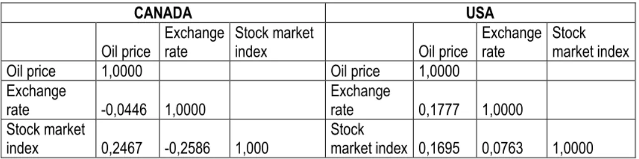
III.3 Correlation matrix

Table 5 presents the correlation matrix for series of the two countries. We can see that except correlation coefficients of Canada between the oil price and the exchange rate on one side, and the stock market index and the exchange rate on the other side, all coefficients are positive.

Table 5 Correlation matrix

CANADA USA

Oil price Exchange rate Stock market index Oil price Exchange rate Stock market index

Oil price 1,0000 Oil price 1,0000

Exchange

rate -0,0446 1,0000 Exchange rate 0,1777 1,0000 Stock market

(43)

29

IV. Empirical results

In order to see if there is a transmission of volatility and detect its direction if so, we estimate a multivariate BEKK GARCH. We focus on the equations h11t, h22t and h33t, which respectively describe

conditional variances of the oil price, the exchange rate and the stock market index: ℎ11𝑡 = 𝑎112 + (𝑏112 𝜀1𝑡−12 + 2𝑏11𝑏211𝑡−1 2𝑡−1+ 𝑏212 𝜀2𝑡−12 + 2𝑏11𝑏311𝑡−1 3𝑡−1 + 2𝑏21𝑏312𝑡−1 3𝑡−1+ 𝑏312 𝜀3𝑡−12 ) + (𝑐112 ℎ11𝑡−1+ 𝑐11𝑐21ℎ12𝑡−1 + 𝑐₁₁𝑐₃₁ℎ_13𝑡−1+ 𝑐₁₁𝑐₂₁ℎ_21𝑡−1+ 𝑐₂₁2 _ℎ 22𝑡−1+ 𝑐21𝑐31ℎ23𝑡−1 + 𝑐11𝑐31ℎ31𝑡−1+ 𝑐21𝑐31ℎ32𝑡−1+ 𝑐312 ℎ33𝑡−1) ℎ_22𝑡 = 𝑎₁₂2 _{+ 𝑎} 222 + (𝑏₁₂2 _𝜀 1𝑡−12 + 2𝑏12𝑏221𝑡−1 2𝑡−1+ 𝑏222 𝜀2𝑡−12 + 2𝑏12𝑏321𝑡−1 3𝑡−1 + 2𝑏₂₂𝑏₃₂_2𝑡−1 _3𝑡−1+ 𝑏₃₂2 _𝜀 3𝑡−12 ) + (𝑐122 ℎ11𝑡−1+ 𝑐12𝑐22ℎ12𝑡−1 + 𝑐₁₂𝑐₃₂ℎ_13𝑡−1+ 𝑐₁₂𝑐₂₂ℎ_21𝑡−1+ 𝑐₂₂2 _ℎ 22𝑡−1+ 𝑐22𝑐32ℎ23𝑡−1 + 𝑐₁₂𝑐₃₂ℎ_31𝑡−1+ 𝑐₂₂𝑐₃₂ℎ_32𝑡−1+ 𝑐₃₂2 _ℎ 33𝑡−1) ℎ_33𝑡 = 𝑎₃₃2 _{+ (𝑏} 132 𝜀1𝑡−12 + 2𝑏13𝑏231𝑡−1 2𝑡−1+ 𝑏232 𝜀2𝑡−12 + 2𝑏13𝑏331𝑡−1 3𝑡−1 + 2𝑏₂₃𝑏₃₃_2𝑡−1 _3𝑡−1+ 𝑏₃₃2 _𝜀 3𝑡−12 ) + (𝑐132 ℎ11𝑡−1+ 𝑐13𝑐23ℎ12𝑡−1 + 𝑐₁₃𝑐₃₃ℎ_13𝑡−1+ 𝑐₁₃𝑐₂₃ℎ_21𝑡−1+ 𝑐₂₃2 _ℎ 22𝑡−1+ 𝑐23𝑐33ℎ23𝑡−1 + 𝑐₁₃𝑐₃₃ℎ_31𝑡−1+ 𝑐₂₃𝑐₃₃ℎ_32𝑡−1+ 𝑐₃₃2 _ℎ 33𝑡−1)

Where 𝜀1,𝑡−12 , 𝜀2,𝑡−12 and 𝜀3,𝑡−12 in each equation represent the effect of news, i.e. an unexpected

change or shock coming from respectively the oil price, the exchange rate and the stock market index in period time t-1.

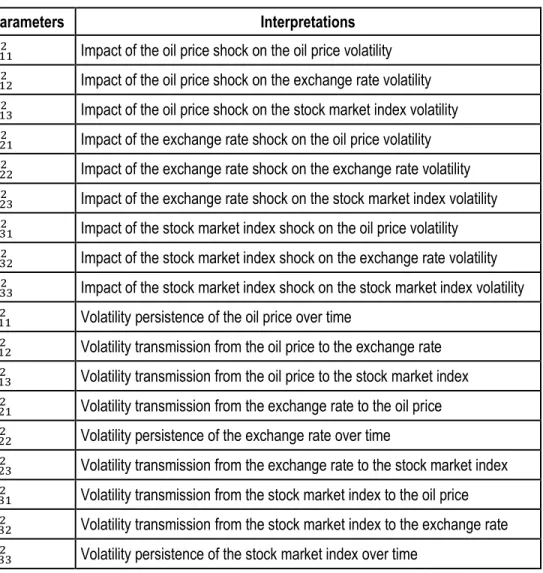
Parameters to interpret in order to see how shocks and volatility are transmitted over time and across the three series are presented as follows:

(44)

30

Table 6 Parameters with their respective interpretations

Parameters Interpretations

𝑏₁₁2 _{Impact of the oil price shock on the oil price volatility}

𝑏₁₂2 _{Impact of the oil price shock on the exchange rate volatility}

𝑏₁₃2 _{Impact of the oil price shock on the stock market index volatility}

𝑏₂₁2 _{Impact of the exchange rate shock on the oil price volatility}

𝑏₂₂2 _{Impact of the exchange rate shock on the exchange rate volatility}

𝑏232 Impact of the exchange rate shock on the stock market index volatility

𝑏₃₁2 _{Impact of the stock market index shock on the oil price volatility}

𝑏₃₂2 _{Impact of the stock market index shock on the exchange rate volatility}

𝑏₃₃2 _{Impact of the stock market index shock on the stock market index volatility}

𝑐₁₁2 _{Volatility persistence of the oil price over time}

𝑐₁₂2 _{Volatility transmission from the oil price to the exchange rate}

𝑐₁₃2 _{Volatility transmission from the oil price to the stock market index}

𝑐₂₁2 _{Volatility transmission from the exchange rate to the oil price}

𝑐222 Volatility persistence of the exchange rate over time

𝑐₂₃2 _{Volatility transmission from the exchange rate to the stock market index}

𝑐₃₁2 _{Volatility transmission from the stock market index to the oil price}

𝑐₃₂2 _{Volatility transmission from the stock market index to the exchange rate}

𝑐₃₃2 _{Volatility persistence of the stock market index over time}

For all of these parameters, the reaction of the other variable is at time t, while the change or the shock in the first variable is at time t-1.

(45)

31

IV. 1. Results for the entire sample

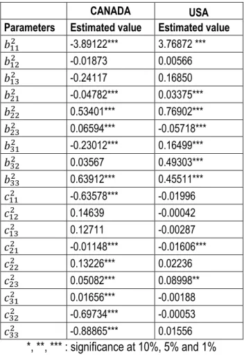
Table 7 presents the results of the model estimated for the two countries:

Table 7 Results of BEKK MGARCH estimations for Canada and USA

CANADA _USA

Parameters Estimated value Estimated value 𝑏₁₁2 _-3.89122*** _{3.76872 ***} 𝑏₁₂2 _-0.01873 _0.00566 𝑏₁₃2 _-0.24117 _0.16850 𝑏₂₁2 _-0.04782*** _0.03375*** 𝑏222 0.53401*** 0.76902*** 𝑏₂₃2 _0.06594*** _-0.05718*** 𝑏₃₁2 _-0.23012*** _0.16499*** 𝑏322 0.03567 0.49303*** 𝑏₃₃2 _0.63912*** _0.45511*** 𝑐112 -0.63578*** -0.01996 𝑐₁₂2 _0.14639 _-0.00042 𝑐₁₃2 _0.12711 _-0.00287 𝑐₂₁2 _-0.01148*** _-0.01606*** 𝑐₂₂2 _0.13226*** _0.02236 𝑐₂₃2 _0.05082*** _0.08998** 𝑐₃₁2 _0.01656*** _-0.00188 𝑐₃₂2 _-0.69734*** _-0.00053 𝑐332 -0.88865*** 0.01556 *, **, *** : significance at 10%, 5% and 1%

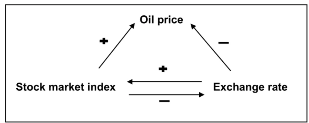
Results of Table 4 show that there is volatility transmission between these variables.

For Canada, we see that an increase of 1% in the volatility of the exchange rate leads to a significant increase of the stock market index volatility for 0.05% (𝑐₂₃2 _{) and a significant decrease of the oil price}

volatility for 0.01% (𝑐₂₁2 _{). We remark also that an increase of 1% in the volatility of the stock market}

index leads to a significant increase of the oil price volatility for 0.02% (𝑐₃₁2 _{) and a significant decrease}

of the exchange rate volatility for 0.7% (𝑐₃₂2 _).

(46)

32

- a bidirectional transmission of volatility between the exchange rate and the stock market index (the transmission from the exchange rate to the stock market index is positive, while it is negative in the opposite direction);

- a unidirectional and positive transmission of volatility from the stock market index to the oil price;

- a unidirectional and negative transmission of volatility from the exchange rate to the oil price. Figure 3 Volatility transmission in Canada

Oil price

Stock market index Exchange rate

This result is consistent with some of the studies presented in the literature review. The unidirectional and positive transmission of volatility from the stock market index to the oil price is consistent with the results of Liu et al. (2013), Aloui et al. 2008 (for Canada) and Malik and Ewing 2009 (for the financial, industrial and consumption sectors). The bidirectional transmission of volatility between the exchange rate and the stock market index is consistent with the study of Zhao (2010). Note that results of Chkili et al. (2012) and Caporale et al. 2013 (Canada and the USA results for the crisis period) also show a bidirectional transmission, but the sign is positive in the two directions, while for our study this is not the case.

These results can be explained as follows:

- For the bidirectional transmission of volatility between the exchange rate and the stock market index, we begin first by explaining the negative sign of the transmission from the stock market index to the exchange rate. This may be justified by the negative correlation between these two variables, highlighting the «safe haven» property of exchange rate investments against stocks. So, the extreme fluctuations of the stock market index during our period lead to an increase of investments on exchange rate. Hence, when the value of the Canadian dollar

(47)

33

increases (i.e. the exchange rate has decreased), this leads to a lower volatility of the exchange rate.

In the opposite direction, the sign of the transmission is positive. This may be explained by the fact that uncertainty in the exchange rate influence the market power of Canadian firms’ products in international markets and hence quantities of exports. Uncertainty in these quantities leads to uncertainty in profits of firms; therefore the volatility of the stock price is affected.

- The transmission of volatility from the stock market index to the oil price may be positive because the period of the financial crisis seems to coincide with the oil shock. So, investors in the oil market become more sensitive to uncertainty information coming from financial market. - The unidirectional and negative transmission of volatility from the exchange rate to the oil price

may be justified by the low volatility of the Canadian exchange rate during our analysis period, while there was an oil shock. That’s why investors become more sensitive to a decrease of volatility in the exchange rate.

Otherwise, coefficients of error terms indicate that the stock market index volatility is affected significantly and positively by a positive shock coming from the exchange rate (𝑏₂₃2 _{). The oil price}

volatility is significantly and negatively affected by a positive shock in the exchange rate and the stock market index (𝑏₂₁2 _and_𝑏

312 ).

Coefficients 𝑐₁₁2 _,_𝑐

222 and 𝑐332 show that there is a significant persistence of volatility over time for the

three variables. For the oil price and the stock market index, this persistence is negative, while for the exchange it is positive.

For the USA, results of the estimation show that the conditions for covariance stationarity are not satisfied, as the sum of all parameters is not less than 1. This suggests that a tendency for volatility do not decay over time. Because of that, we can’t use results of this estimation to make conclusions about volatility transmission.

IV. 2. Sub sample results

In order to check the stability of these results, we divide the analysis period in three sub periods. This division is made based on the two major crises during the decade 2000-2010. The first is the stock market crash of 2001-2002 and the second is the financial crisis of 2008.