HAL Id: hal-00366617
https://hal.archives-ouvertes.fr/hal-00366617
Submitted on 9 Mar 2009HAL is a multi-disciplinary open access
archive for the deposit and dissemination of sci-entific research documents, whether they are pub-lished or not. The documents may come from
L’archive ouverte pluridisciplinaire HAL, est destinée au dépôt et à la diffusion de documents scientifiques de niveau recherche, publiés ou non, émanant des établissements d’enseignement et de
An eXtended Stochastic Finite Element Method for
solving stochastic partial differential equations on
random domains
Anthony Nouy, Alexandre Clement, Franck Schoefs, N. Moes
To cite this version:
Anthony Nouy, Alexandre Clement, Franck Schoefs, N. Moes. An eXtended Stochastic Finite Element Method for solving stochastic partial differential equations on random domains. Com-puter Methods in Applied Mechanics and Engineering, Elsevier, 2008, 197 (51-52), pp.4663-4682. �10.1016/j.cma.2008.06.010�. �hal-00366617�
An eXtended Stochastic Finite Element
Method for solving stochastic partial
differential equations on random domains
A. Nouy ∗ , A. Cl´ement, F. Schoefs, N. Mo¨es
Research Institute in Civil Engineering and Mechanics (GeM), Nantes Atlantic University, Ecole Centrale Nantes, UMR CNRS 6183, 2 rue de la Houssini`ere,
B.P. 92208, 44322 Nantes Cedex 3, FRANCE
Abstract
Recently, a new strategy was proposed to solve stochastic partial differential equa-tions on random domains. It is based on the extension to the stochastic framework of the eXtended Finite Element Method (X-FEM). This method leads by a “direct” calculus to an explicit solution in terms of the variables describing the random-ness on the geometry. It relies on two major points: the implicit representation of complex geometries using random level-set functions and the use of a Galerkin ap-proximation at both stochastic and deterministic levels. In this article, we detail the basis of this technique, from theoretical and technical points of view. Several numerical examples illustrate the efficiency of this method and compare it to other approaches.
Key words: Computational Stochastic Mechanics, Stochastic Partial Differential Equations, Random domain, eXtended Finite Element Method, Stochastic Finite Element, Polynomial Chaos
1 Introduction
Computer simulations of mechanical models, supported by the availability of enhanced computational resources, take today a very significant place in decision-makings which can have major consequences in economic or human terms. In a structural analysis, the incorporation of uncertainties inherent in
∗ Corresponding author. Tel.: +33(0)2-51-12-55-20; Fax: +33(0)2-51-12-52-52 Email address: anthony.nouy@univ-nantes.fr (A. Nouy).
the model, related to material properties, loadings or geometry, seems today essential if one seeks to obtain “reliable” numerical predictions, usable in a design process or a decision-making. This necessity led to a rapid development of many ad hoc numerical methods, such as stochastic finite elements methods [1–3]. These methods provide high quality predictions which are explicit in terms of the random variables describing the uncertainties. The increase in their performances, due to the development of ad hoc resolution techniques [4,6–8], allows expecting their use in many domains of applications such as structural design, reliability analysis, etc. The incorporation of uncertainties on material properties or loadings is quite well mastered within the framework of these techniques. However, there is still no available efficient strategy to deal with uncertainties on the geometry although it could have a great interest in various applications.
A natural way to solve a stochastic problem defined on a random domain con-sists in using a classical stochastic finite element method with remeshings, such as Monte-Carlo simulations [9,10], response surface method, projection [11] or regression [12] methods. These techniques only require the use of a simple deterministic finite element calculation code. However, they require numerous deterministic computations, each of which requiring the construction of a new conforming mesh, which leads to prohibitive computational costs.
In order to avoid remeshings and to obtain an “explicit” description of the stochastic solution, a possible alternative technique consists in building a clas-sical finite element approximation on a reference deterministic domain, and to introduce a random mapping between this domain and the random domain. This technique can also be seen as a classical finite element technique on a random mesh. Such a strategy has been used in [13,14] and also in [5] for the case of random interfaces in layered media. The main difficulty lies in the construction of a suitable random mapping in the case of complex geometries.
Recently, a new stochastic finite element method was proposed for solving partial differential equations on random domains [15]. This technique, called eXtended Stochastic Finite Element method (X-SFEM), is based on an ex-tension to the stochastic framework of the X-FEM method [16,17]. It relies on two major points. The first one consists in representing the geometry in an implicit way by using the level-set technique [18]. The random domain is then characterized by the negative set of a random level-set function, which is defined on a fictitious deterministic domain containing all outcomes of the physical domain. The second point consists in using a Galerkin approxima-tion technique at both deterministic and stochastic levels. A tensor product approximation is made possible by considering prolongation of functions on the fictitious domain. The resulting technique does not require any remeshing and allows the handling of complex geometries. Another advantage is that it leads to a solution which is explicit in terms of the basic random variables
de-scribing the geometry, thus allowing an easy post-processing of the stochastic solution at a very low cost.
In this paper, we introduce the basis of the X-SFEM method from a theo-retical point of view and also focus on technical aspects. The method will be presented in the context of linear elasticity. However, the mathematical results and the proposed methodology could be applied to more general linear ellip-tic stochasellip-tic partial differential equations defined on random domains. Here, we only deal with random shapes. This is a degenerated case of the X-FEM method [19,20] where only a classical finite element approximation can be used at the space level, without enrichment of the approximation space by the partition of unity method [21]. Let us mention that fictitious domain methods [22–25], recently extended to the stochastic framework [26], start with similar reformulation of the problem and definition of approximation spaces. How-ever, the methodology proposed in this article differs by the representation of the geometry and the underlying computational aspects (construction and resolution of the discretized problem).
The outline of the paper is as follows. In section 2, we introduce the strong and weak formulations of a linear elasticity problem defined on a random domain. In section 3, we briefly recall the basis of stochastic finite element methods in the case of a deterministic domain. It allows us to point out why their extension in the case of a random domain is not straightforward and also to introduce some useful notations. In section 4, we present possible finite element strategies to deal with random domains and point out some of their drawbacks. Section 5 is devoted to the presentation of the X-SFEM method from a theoretical point of view. In particular, we focus on the mathemati-cal interpretation of the approximation based on a Galerkin projection and compare it to other projection methods. Section 6 details the computational aspects of the X-SFEM method: construction and resolution of the discretized problem. In particular, we illustrate that the construction of the discretized problem requires the development of a specific numerical integration technique at the stochastic level. For that purpose, a general numerical procedure is pro-posed, which consists in building suitable partitions of the stochastic domain and using a Gaussian quadrature on each subdomain. Finally, in section 7, three numerical examples illustrate several aspects of the X-SFEM method: quality of the Galerkin approximation, influence of the proposed stochastic integration procedure and efficiency of the resolution strategy. The method is systematically compared to other approaches. In particular, it is compared to a stochastic L2 projection method based on X-FEM.
2 Formulation of the problem
2.1 The deterministic problem
In this article, we will focus on the analysis of the deformation of a structure under small perturbations assumption. We consider that the structure occu-pies a domain Ω ⊂ Rd (see figure 1). It is submitted to body loads f (x) on Ω and surface loads F (x) on a part Γ2 of the boundary ∂Ω. The structure is fixed on a part Γ1 of the boundary ∂Ω such that Γ1∩ Γ2 = ∅. The complemen-tary part of Γ1∪ Γ2 in ∂Ω, denoted by Γ0, is considered as a free boundary. We denote by u(x) the displacement field, ε(u) the symmetric part of the displacement gradient (i.e. the strain tensor) and by σ the stress tensor. In this article, we will consider the case of a linear elastic material and denote by C the Hooke fourth-order tensor. The strong formulation of the problem writes: find (u, σ) such that
div σ+ f = 0 on Ω, σ = C : ε(u) on Ω, σ· n = F on Γ2, σ· n = 0 on Γ0, u= 0 on Γ1. (1)
where n is the unit outward normal to the boundary.
Ω F
f
Γ2
Γ1
Fig. 1. Model problem
2.2 The stochastic problem
Now, we consider that the structure occupies a random domain. For the sake of generality, we also consider that material properties and loads can be random. Let us suppose that the probability space (Θ, B, P ) allows the representation
of the probabilistic content of the problem. Θ is the set of elementary events, B a σ-algebra on Θ and P a probability measure. An element θ ∈ Θ is an elementary event. The random domain can be characterized by the random variable Ω : θ ∈ Θ 7→ Ω(θ) ⊂ Rd. Ω(θ) represents an outcome of the domain. Figure 2 illustrates two outcomes of the random domain and of the associated parts of its boundary.
Γ (θ ) 1 1 Γ (θ ) 1 2 Ω(θ ) 1 Ω(θ ) 2 Γ (θ ) 2 2 Γ (θ ) 2 1
Fig. 2. Two outcomes of the random domain Ω(θ) and associated parts of boundary Γ1(θ) and Γ2(θ).
Then, the strong formulation of the stochastic problem writes: find random fields u and σ which verify P -almost surely the set of equations (1). We recall that a property is P -almost sure if the probability of the event “the property is false” is zero.
2.3 Weak formulation of the stochastic problem
Let us first introduce a classical weak formulation at the space level: find u such that ∀θ ∈ Θ, u(·, θ) ∈ U(θ) = {v ∈ (H1(Ω(θ)))d; v = 0 on Γ1(θ)}, and such that we have P -almost surely
a(u(·, θ), v; θ) = b(v; θ) ∀v ∈ U(θ), (2)
where a(·, ·; θ) is a continuous symmetric coercive bilinear form on U(θ) and b(·; θ) is a continuous linear form on U(θ), defined by
a(u, v; θ) = Z Ω(θ) ε(v) : C : ε(u) dx, (3) b(v; θ) = Z Ω(θ)f · v dx + Z Γ2(θ) F · v ds. (4)
Then, a weak formulation at both space and stochastic levels can be intro-duced. We consider that the problem can be formulated in the following
func-tion space: V= {u : θ ∈ Θ 7→ u(·, θ) ∈ U(θ); Z Θkuk 2 U(θ)dP(θ) < ∞} := L2(Θ, dP ; U). (5)
The weak formulation then writes : find u ∈ V such that
A(u, v) = L(v) ∀v ∈ V, (6) where A(u, v) = Z Θa(u, v; θ) dP (θ) := E(a(u, v; θ)), (7) L(v) = Z Θb(v; θ) dP (θ) := E(b(v; θ)). (8) E(·) denotes the mathematical expectation. We will consider that bilinear form A is continuous and coercive on V and that linear form L is continuous on V, such that problem (6) is well posed. In the case of a deterministic domain, the reader can refer to [2,27] for a detailed and comprehensive study of the regularity requirements on the data (C, f and F ) leading to the desired properties. To the knowledge of the authors, stochastic problem (6) has not been deeply studied from a mathematical point of view in the case of random domains. In particular, regularity requirements on the random domain should be further analyzed. These mathematical aspects are beyond the scope of this article. Some mathematical results on the effects of uncertainties in the domain can be found in [28,29].
Remark 1 Coercivity and continuity properties of A and L are inherited from those of a and b: ∀u, v ∈ U(θ), |a(u, v; θ)| 6 CakukU(θ)kvkU(θ), a(v, v; θ) > αakvk2U(θ), and |b(v; θ)| 6 CbkvkU(θ), where Ca, Cb < ∞ and αa > 0. These three constants depends on material properties, loads and also on the geom-etry. If there exists such constants Ca, Cb and αa independent of the event θ, coercivity and continuity properties of A and L follows with the same con-stants.
2.4 Stochastic modeling and discretization
In practice, we generally consider that the probabilistic content of the stochas-tic problem can be represented by a finite set of random variables ξ : Θ → Rm. This is the case when material properties, loads and geometry depend on a finite set of parameters which are random variables. When these parameters are stochastic fields, a preliminary step is usually performed in order to dis-cretize these parameters (e.g. by Karhunen-Loeve decomposition [30,31,1]) and represent them in terms of a finite set of random variables.
Let us now consider that the data of stochastic problem (6) can be written in terms of ξ, so that bilinear form a and linear form b can also be written in terms of ξ: a(·, ·; θ) ≡ a(·, ·; ξ(θ)), b(·; θ) ≡ b(·; ξ(θ)). Then, by the Doob-Dynkin’s lemma [32], we have that the solution of problem (6) can be written in terms of ξ, i.e. u(·, θ) ≡ u(·, ξ(θ)). The stochastic problem can then be reformulated in the m-dimensional image probability space (Θ, B, Pξ), where Θ ⊂ Rm is the range of ξ and Pξ the probability measure associated with ξ (see e.g. [2] for details). Function space (6) is now replaced by
V= {u : ξ ∈ Θ 7→ u(·, ξ) ∈ U(ξ); E(ku(·, ξ)k2U
(ξ)) < ∞}. (9)
In the definition of function space V and of bilinear form A and linear form L, the mathematical expectation must be interpreted as E(f (ξ)) =RΘf(y)dPξ(y).
In what follows, we will mainly use the initial probability space (Θ, B, P ). The reader must keep in mind that at each moment, the elementary event θ ∈ Θ can be replaced by ξ ∈ Θ in the expression of any random function.
3 Stochastic finite element methods in the case of a deterministic domain
Before introducing some classical techniques to deal with random domains, we briefly recall the basis of stochastic finite element methods in the case of a deterministic domain (see e.g. [1–3,33]). It will allow us to introduce some useful notations and to point out why their extension in the case of a random domain is not straightforward.
Here, we suppose that the domain Ω and the associated parts of its boundary Γi are deterministic. In this case, function space U does not depend on the elementary event θ. Then, function space V has a tensor product structure:
V= L2(Θ, dP ; U) ∼= L2(Θ, dP ) ⊗ U := S ⊗ U, (10)
where S = L2(Θ, dP ) is the space of second order real-valued random variables. Classical stochastic finite elements methods then introduce a tensor product approximation as follows.
3.1 Approximation at the space level
At the space level, we introduce a finite element approximation space Uh defined by Uh = {v(x) = N X i=1 ϕi(x)vi = ϕ(x)v, v ∈ RN}, (11)
where the ϕi(x) ∈ U are the finite element basis functions associated with a mesh Th of domain Ω. A semi-discretized approximation space Vh ⊂ V can then be defined as follows:
Vh = S ⊗ Uh = {v(x, θ) = N X i=1 ϕi(x)vi(θ) = ϕ(x)v(θ), v ∈ S ⊗ RN}. (12)
The semi-discretized approximate solution uh ∈ Vh of problem (6) is defined by:
A(uh, vh) = L(vh) ∀vh ∈ Vh. (13) Problem (13) can be written under the following matrix strong form: find u : θ 7→ u(θ) ∈ RN such that we have P -almost surely
A(θ)u(θ) = b(θ), (14) where random matrix A and random vector b are defined by:
(A(θ))ij = a(ϕj, ϕi; θ), (15) (b(θ))i = b(ϕi; θ). (16)
3.2 Approximation at the stochastic level
Several choices have been proposed for the construction of a basis of the space of second order random variables S = L2(Θ, dP ): polynomial chaos [1,34], gen-eralized polynomial chaos [35,36], h-p finite elements [37] or wavelets [38,39]. Let {Hα}α∈Ibe such a basis, where I denotes a countable set of indices. Then, we can naturally introduce a finite dimensional approximation space SP ⊂ S, defined by
SP = {v(θ) = X α∈IP
vαHα(θ), vα ∈ R}, (17)
where IP is a subset of P indices in I. In the following, we will suppose that the Hα are orthonormal, i.e. E(HαHβ) = δαβ.
Let us illustrate the construction of the generalized polynomial chaos approx-imation [35,36], which will be used in numerical examples. We consider, as in section 2.4, that the probabilistic content of the problem is represented by m random variables (ξ1, . . . , ξm) := ξ. For the construction of chaos basis associ-ated with an arbitrary probability measure, the reader can refer to [36]. Here, we will consider that random variables are statistically independent (property possibly obtained by a suitable mapping). Let (Θ, B, Pξ) be the associated im-age probability space. The space L2(Θ, dPξ) of second order random variables on Θ has a tensor product structure: L2(Θ; dPξ) = ⊗m
j=1L2(Θ(j), dPξj), where
Θ(j) ⊂ R is the range of random variable ξ
j and Pξj the associated marginal
probability measure. Basis functions Hα are then taken as multi-dimensional orthonormal polynomials. A simple way to define the Hα is to use a tensor product basis. Let us denote by I = {α = (α1, . . . , αm) ∈ Nm} the set of m-dimensional multi-indices. Then, denoting by {h(j)k }k>0 the set of orthonor-mal polynomials in L2(Θ(j), dP
ξj), where index k denotes the degree of the
polynomials, the Hα are simply defined as follows: Hα(ξ) =Qmj=1h(j)
αj(ξj). The
approximation space SP can then be defined by selecting the multi-dimensional polynomials with total degree less than p. It consists in taking the following subset of indices IP = {α ∈ I;Pmi=1αi 6p}. In this case, the number of basis functions is P = (m+p)!m!p! .
Finally, a tensor product approximation space Vh,P ⊂ V is classically defined as follows: Vh,P = SP ⊗ Uh (18) = {v(x, θ) = N X i=1 X α∈IP ϕi(x)Hα(θ)vi,α, vi,α ∈ R} = {v(x, θ) = ϕ(x)v(θ), v(θ) ∈ SP ⊗ RN}.
3.3 Definition of the approximation
Many choices are possible for the definition of an approximation in Vh,P. Be-low, we present the more commonly used definitions, namely the stochastic Galerkin method and the classical projection method.
3.3.1 Stochastic Galerkin method
A classical way to define the approximate solution uh,P ∈ Vh,P consists in injecting the approximation space Vh,P in the weak formulation (6). It leads
to the so-called Galerkin approximation which solves
A(uh,P, vh,P) = L(vh,P) ∀vh,P ∈ Vh,P, (19)
which is equivalent to the following system of N × P equations:
X
α∈IP
E(HβAHα)uα = E(bHβ) ∀β ∈ IP. (20)
3.3.2 Projection method
The projection method consists in defining the approximate solution as the projection on Vh,P of the semi-discretized solution with respect to a suitable inner product. A classical choice consists in using the natural L2 inner product on V, defined by ≪ u, v ≫L2= Z Θ Z Ω u· v dx dP (θ). (21)
Denoting by uh(x, θ) = ϕ(x)u(θ) ∈ Vh the semi-discretized solution, which solves (13), the approximation uh,P ∈ Vh,P is then defined by:
≪ uh,P, vh,P ≫L2=≪ uh, vh,P ≫L2 ∀vh,P ∈ Vh,P. (22)
Equation (22) is equivalent to the following definition of the coefficients of the approximation:
uα =
Z
ΘHα(θ)u(θ)dP (θ) = E(Hαu). (23) We emphasize on the fact that this equivalence comes from the tensor product structure of the approximation and of the particular choice of inner product. The expectation can then be computed by a suitable numerical integration at the stochastic level (quadrature, Monte-Carlo, etc.), which writes
uα ≈X k
ωkHα(θk)u(θk), (24)
where the θk are the integration points (particular elementary events) and the ωk the associated integration weights. For each integration point, comput-ing u(θk) = A−1(θk)b(θk) requires solving a classical deterministic problem. In this case, the projection method is said to be non-intrusive since it only requires the use of a simple deterministic code for each integration point. How-ever, computational costs are generally prohibitive since this technique often necessitates a large number of integration points in order to obtain a good ac-curacy on the coefficients. Let us mention that sparse quadrature techniques have been proposed in order to reduce the number of integration points [3].
4 Classical stochastic finite elements to deal with random domains
The question is now: how to define an approximation of problem (6) in the case of a random domain ? The extension of classical stochastic finite element methods presented in section 3 is not straightforward since V, defined in (5), has no more a tensor product structure. In the following, we recall two possible strategies to construct stochastic finite element approximations in the case of a random domain.
4.1 Classical finite element techniques with remeshings
A natural way to solve a stochastic problem defined on a random domain consists in using a classical stochastic finite element method with remeshings, such as Monte-Carlo simulation [9,10], response surface method, projection [11] or regression [12] methods. These techniques require solving problem (2) for given elementary events θk ∈ Θ. The meaning of these points depends on the method which is used: random samplings for Monte-Carlo, stochas-tic integration points for projection method, etc. These techniques have the great advantage that they only require the use of a simple deterministic finite element calculation code.
For a given elementary event θk ∈ Θ, we introduce a new finite element mesh Th(θk) of the domain Ω(θk) and an associated finite element approximation space Uh(θk) ⊂ U(θk) defined by Uh(θk) = {vh(x) = PN (θk)
i=1 ϕi(x, θk)vi, vi ∈ R}. The mesh, and then the basis functions ϕi(x, θk) ∈ Uh(θk), clearly depend on the elementary event θk.
The first drawback of these techniques is that they require numerous deter-ministic computations, each of which requiring the following classical steps: remeshing of the domain, assembling and solving a finite element problem of type (14). Another main drawback is that outcomes of the solution uh(·, θk) ∈ Uh(θk) are defined on different meshes and that corresponding finite ele-ment problems (14) have a different algebraic structure. Information on non-computed outcomes is then unreachable. Moreover, an a posteriori proba-bilistic characterization of the solution is generally prohibitive since it would require storing the meshes and finite element solutions for all computed ele-mentary events.
Of course, it is possible to focus on a mesh and geometry independent quan-tity of interest. Let us denote by J(uh(·, θ)) this quanquan-tity of interest and by J(uh(·, θk)) its computed outcomes. In the context of Monte-Carlo simula-tions, these outcomes allow evaluating statistics of J. In the case of projection methods (see section 3.3.2), outcomes correspond to stochastic integration
points which are used to compute the decomposition of J on a stochastic basis: J =Pα∈IJαHα(θ), with
Jα = E(HαJ(uh)) ≈
X
k
ωkHα(θk)J(uh(·, θk)). (25)
The problem is that these quantities of interest are not necessarily known a priori, before having an idea of the solution.
4.2 Finite element approximation on a random mesh
In order to avoid remeshings and to obtain an “explicit” description of the stochastic solution, an alternative technique consists in building a classical finite element approximation on a reference deterministic domain, and to in-troduce a random mapping between this domain and the random domain Ω(θ). Such a strategy has been used in [13,14]. Let us briefly describe this methodology in our context to point out its advantages and drawbacks.
4.2.1 Description of the random geometry by a random mapping
We first introduce a reference deterministic domain Ω0 ⊂ Rdand suppose that there exists a continuous one to one mapping T (·, θ) between Ω0 and the out-come Ω(θ) of the random domain: T (·, θ) : x0 ∈ Ω0 7→ x = T (x0, θ) ∈ Ω(θ). We denote by T∗(·, θ) the inverse mapping. Reference domain Ω0 and mapping T allow the description of the random domain Ω. We suppose that the parts Γi(θ) of boundary ∂Ω(θ) are the images by mapping T (·, θ) of complementary parts Γ0i of ∂Ω0. We denote by T|i the restriction of T on Γ0i.
4.2.2 Construction of an approximation space
We introduce a fixed finite element mesh T0
h of reference domain Ω0, leading to the definition of the following finite element approximation space: U0
h = {v0(x0) =PN
i=1ϕ0i(x0)vi, vi ∈ R}, where the ϕ0i ∈ U0 = {v ∈ (H1(Ω0))d; v = 0 on Γ0
1} are the finite element basis functions associated with the mesh T0h. Approximation space U0
h being independent of the event, a tensor product approximation space can be introduced: V0
h,P ∼= SP ⊗ U0h. An approximation subspace Vh,P of V is then simply defined by a suitable mapping of functions in V0 h,P: Vh,P = {v(x, θ) = v0(T∗(x, θ), θ), v0 ∈ V0 h,P} (26) = {v(x, θ) = N X i=1 ϕi(x, θ)vi(θ), vi(θ) ∈ SP},
where ϕi(x, θ) = ϕ0i(T∗(x, θ)). The image of T0h by mapping T (·, θ) is a mesh of Ω(θ), denoted by Th(θ), which can be considered as a random mesh.
4.2.3 Definition and construction of the approximation
At this point, different definitions of the approximation can still be used, as introduced in section 3.3. The approximation uh,P ∈ Vh,P can be written uh,P = ϕ(x, θ)u(θ), with u(θ) = Pα∈IP uαHα(θ). The standard Galerkin
ap-proximation is still defined by problem (19). Although the apap-proximation has not a tensor product structure, coefficients uα ∈ RN are still defined by the system of equations (20), where components of random matrix A and random vector b can be written as integral on the reference domain. For every func-tion f (x, θ), with x ∈ Ω(θ), let f0(x0, θ) = f (T (x0, θ), θ) be the corresponding function defined on Ω0× Θ. Then, components of A and b write:
(A(θ))ij = a(ϕj, ϕi; θ) = Z Ω0ε(ϕ 0 i) : C0 : ε(ϕ0j) J0dx0, (27) (b(θ))i = b(ϕi; θ) = Z Ω0ϕ 0 i · f0 J0dx0+ Z Γ0 2 ϕ0i · F0 J20ds0, (28) where J0 and J0
2 are the jacobians of mappings T and T|2 respectively. In equation (27), the strain term can be written as follows: ε(ϕ0
j) = 12( ∂ϕ0 j ∂x + ∂ϕ0 j ∂x T ), with ∂ϕ0j ∂x = ∂ϕ0 j ∂x0 · ³ ∂T ∂x0 ´−1
. The randomness on the geometry is then only contained in mappings T and T|2and their jacobians. However, the integration of the left and right-hand sides of system (20) is not so trivial and necessitates a particular attention. An a priori explicit stochastic representation of the mappings can facilitate this integration.
Another definition of the approximation, based on a projection method, can also be used. It still consists in defining the random vector u ∈ RN ⊗ SP by equations (23) and (24). However, in this case, the approximation uh,P appears to be the projection of the semi-discretized solution with respect to the following inner product on V:
≪ u, v ≫ = Z Θ Z Ω(θ)u· v(J 0)−1dx dP(θ) = Z Θ Z Ω0u 0· v0dx dP(θ). (29) 4.2.4 Remarks
Compared to classical finite element techniques with remeshings, this method has the advantage to do not require any remeshing. It also leads to a complete description of the stochastic solution. However, some drawbacks can be pointed
out. First, the construction of mapping T is not so trivial and necessitates the elaboration of ad-hoc numerical techniques [40,13]. Regularity requirements on the random mapping avoid dealing with general random domains, and in particular with topology changes. Moreover, since the approximation space has not a tensor product structure, a simple post-processing of random vector u does not give meaningful information on the solution. For example, the expectation E(u) leads to the expectation of u0(x0, θ) but not the expectation of the physical displacement field u(x, θ) at a given point x.
5 The eXtended Stochastic Finite Element Method (X-SFEM)
In this section, we present the basic principles of the eXtended Stochastic Finite Element Method (X-SFEM), which is the extension of the X-FEM method in the stochastic framework. In this article, we only deal with random shapes. This is a degenerated case of the X-FEM method [19,20] where only a classical finite element approximation can be used, without enrichment of the approximation space by the partition of unity method. In this section, the method is introduced from a theoretical point of view. Computational aspects related to the construction of the approximation will be detailed in the following section.
5.1 Reformulation of the problem on a deterministic domain
We introduce a deterministic spatial domain B which contains all outcomes of the random domain, i.e. Sθ∈ΘΩ(θ) ⊂ B (figure 3).
B
Ω(θ)
Fig. 3. Deterministic domain B including all outcomes of the random domain Ω(θ)
The problem is then reformulated by considering prolongation of functions of Von B ×Θ. The aim of working in this deterministic domain is to facilitate the construction of approximation spaces, independently of the random geometry. We first introduce the function space
Then, the prolongation of the stochastic solution u will be searched in the following function space
V= {v : θ ∈ Θ → v(·, θ) ∈ U(θ); Z Θkvk 2 U(θ)dP(θ) < ∞} := L2(Θ, dP ; U) (31)
The stochastic problem (6) can now be equivalently reformulated as follows: find u ∈ V such that
A(u, v) = L(v) ∀v ∈ V (32)
where bilinear form A and linear form L are defined as in the initial formulation (6). Bilinear form A is clearly only semi-coercive on V, such that there exists infinitely many solutions of problem (32). However, we can show that the “physical part” of these solutions is unique and coincides with the solution of the initial problem (6) (see [15]). The physical part of a solution u ∈ V is the restriction u|P of u on the physical domain P of B × Θ, defined by
P= {(x, θ) ∈ B × Θ; x ∈ Ω(θ)}. (33)
In other words, all solutions of problem (32) differs by functions whose support is included in the complementary subset of P, which can be called the “non-physical domain”. In the following, we will denote by IP(x, θ) the indicator function of P, defined on B × Θ, which writes
IP(x, θ) = 1 if (x, θ) ∈ P 0 otherwise := IΩ(θ)(x), (34)
where IΩ(θ)(x) is the classical indicator function of spatial domain Ω(θ). Bi-linear form A and Bi-linear form L can be equivalently rewritten as follows:
A(u, v) = Z Θ Z Bε(v) : C : ε(u) IPdx dP(θ), (35) L(v) = Z Θ Z Bv· f IPdx dP(θ) + Z Θ Z Γ2(θ) v· F ds dP (θ). (36)
5.2 Representation of the geometry using random level-sets
5.2.1 Random level-sets
Here, we represent the random geometry in an implicit manner using the level-set technique [18]. The level-level-set technique consists in representing an hyper-surface Γ in Rdby the iso-zero of a function φ called a level-set function. Then,
to represent a random hyper-surface Γ(θ), it is natural to introduce a random level-set function φ(x, θ) such that
Γ(θ) = {x ∈ Rd; φ(x, θ) = 0}. (37) The level-set is generally taken as the signed distance function to the hyper-surface: φ(x, θ) = ±dist(x, Γ(θ)). The distance function have some interesting properties. For example, on the hyper-surface, the gradient of φ with respect to x is the unitary normal to the hyper-surface. Let us note that the dirac measure on Γ(θ), characterized by a level-set φ, can be written δΓ(θ)(x) = δ(φ(x, θ)), where δ is the classical dirac delta function.
Fig. 4. Random level-set φ(x, θ) whose iso-zero represents the boundary of random domain Ω(θ)
Here, the hyper-surface to be represented can be the complete boundary ∂Ω(θ) of domain Ω (figure 4) or a part of this boundary. By convention, we consider that φ(·, θ) takes negative values on random domain Ω(θ) and positive val-ues on the complementary domain in B. The random domain Ω(θ) and its boundary can then be characterized by
Ω(θ) = {x ∈ B; φ(x, θ) < 0}, (38) ∂Ω(θ) = {x ∈ B; φ(x, θ) = 0} ∪ {x ∈ ∂B; φ(x, θ) < 0}. (39)
The indicator function of the physical domain, defined by (34), can then be simply written in terms of the level-set:
IP(x, θ) = IΩ(θ)(x) = H(−φ(x, θ)) (40)
where H : R → {0, 1} is the heaviside function defined by H(y) =
1 if y > 0 0 if y 6 0. In order to define boundary conditions, we also need to describe random parts of the boundary ∂Ω. This description is also greatly simplified by using the level-set technique. Let us see for example how to describe Γ2(θ), where sur-face loads are applied, and how to define integrals on Γ2. Two first cases can be encountered:
• Γ2 = {x ∈ B; φ = 0} : Z Γ2(θ) f ds= Z B f δ(φ) dx (41) • Γ2 = {x ∈ ∂2B; φ < 0} : Z Γ2(θ) f ds= Z ∂2B f H(−φ) ds (42)
In (41), Γ2 is the iso-zero of the level-set φ. In (42), Γ2 = ∂2B∩ Ω, where ∂2B is a deterministic part of the boundary of B. Of course, these cases do not span all the possibilities. For example, a specific treatment is required if Γ2 is only included in the hyper-surfaces described in (41) and (42). A possibility consists in introducing an auxiliary level-set φe whose iso-zero characterizes the boundary of the hyper-surface. If we consider by convention that φe takes negative values on Γ2, that leads to the following two other cases:
• Γ2 = {x ∈ B; φ = 0;φ <e 0} : Z Γ2(θ) f ds= Z B f H(−φ)δ(φ) dxe (43) • Γ2 = {x ∈ ∂2B; φ < 0;φ <e 0} : Z Γ2(θ) f ds= Z ∂2B f H(−φ)H(−φ) dse (44)
The case of equation (43) is illustrated on figure 5.
Γ
2Fig. 5. Level-set eφ(·, θ) whose iso zero on ∂Ω(θ) represents the boundary of hyper– surface Γ2(θ)
5.2.2 On the construction of levels-sets
For some particular shapes (circles, hyper-planes, ellipses, polygones, etc), an explicit expression of level-sets can be used [20]. Then, considering the parameters of these level-sets as random variables (e.g. center coordinates and radius of the circle, etc), we easily define the associated random level-sets.
In the context of the level-set technique, a simple way to obtain more complex geometries consists in using classical boolean operations on basic domains. Let us suppose that Ω1 and Ω2are two random domains, respectively characterized by random level-sets φ1 and φ2. Then, we want to define a random domain Ω, characterized by a random level-set φ, by doing boolean operations on Ω1 and Ω2. Below, we present classical boolean operations and the associated manipulations on level-sets: • union : Ω = Ω1∪ Ω2, φ(x, θ) = min{φ1(x, θ), φ2(x, θ)} (45) • intersection: Ω = Ω1∩ Ω2, φ(x, θ) = max{φ1(x, θ), φ2(x, θ)} (46) • complement: Ω = Ωc 1, φ(x, θ) = −φ1(x, θ) (47)
In this article, we will consider that level-sets are obtained by the above tech-niques and that the probabilistic characterization of these level-sets is given. The question of the probabilistic identification of random level-sets, as well as the representation of more general random shapes by level-sets, will be introduced in a subsequent paper.
5.2.3 Discretization of level-sets
In practice, a level-set is approximated at the space level by introducing a fi-nite element mesh of domain B. This mesh can be different from the one which is used for the approximate solution. However, the use of the same finite el-ement mesh greatly simplifies the computational aspects within the context of X-SFEM. We denote by {ϕi(x)}i∈I the set of finite element interpolation functions associated with the nodes {xi}i∈I of the mesh. A level-set, approx-imated at the space level, writes φ(x, θ) = Pi∈Iϕi(x)φi(θ), where the φi(θ) are the nodal values of the random level-set, which are random variables. In this article, we will consider a linear interpolation for the level-set. The iso-zero of the approximate level-sets is then continuous and piecewise linear, thus approximating the geometry piecewise linearly.
The randomness on the geometry is completely contained in the random level-sets. Level-sets, after the stochastic modeling step (see section 2.4), can be expressed in terms of basic random variables ξ. In some cases, a simple and explicit representation of the level-set in terms of ξ could be available. How-ever, in practice, an approximation of the level-set at the stochastic level can
be convenient from a computational point of view. It consists in decompos-ing the level-set on a suitable stochastic basis (in practice the same as for the approximate solution): φ(x, ξ(θ)) = Pi∈IPαϕi(x)Hα(ξ(θ))φi,α. Giving the coefficients φi,αthen allow a complete characterization of the approximate random geometry and a quick evaluation of outcomes of the random level-set.
5.3 Discussion on boundary conditions
In the case where only Neumann boundary conditions are applied (Γ1 = ∅), V= L2(Θ, dP ; (H1(B))d) has a tensor product structure, i.e. V ∼= L2(Θ, dP )⊗ (H1(B))d. A classical tensor product approximation can then be easily con-structed.
In the case where Dirichlet boundary conditions are applied on the random boundary’s part Γ1, V has no more a tensor product structure. A reformulation of the problem must then be introduced if we want to work in a tensor product function space for the displacement field and then facilitates the construction of approximation spaces. A possible way to achieve this is to introduce a Lagrange multiplier p in order to impose the Dirichlet boundary conditions in a weak sense. The problem can be reformulated as follows: find u ∈ S ⊗ (H1(B))d and p ∈ Q such that ∀v ∈ S ⊗ (H1(B))d and ∀q ∈ Q,
A(u, v) + Z Θ Z Γ1(θ) p· v ds dP (θ) = L(v), (48) Z Θ Z Γ1(θ) q· u ds dP (θ) = 0. (49)
A natural choice consists in introducing a boundary supported Lagrange mul-tiplier, whose function space is defined by
Q= {p : θ 7→ p(·, θ) ∈ H−1/2(Γ1(θ));
Z
Θkp(·, θ)k 2
H−1/2(Γ1(θ))dP(θ) < ∞}. (50)
Although the construction of an approximation space for the displacement field is then greatly simplified, a particular care must still be taken for the choice of the approximation space of Q in order to satisfy the discrete inf-sup condition [41]. In the case where Γ1 is deterministic, Q ∼= S ⊗ H−1/2(Γ1) has a tensor product structure. The construction of approximation spaces can then be made independently at space and stochastic levels. It allows taking part of previous works in the deterministic context for a suitable construction of approximation subspaces of (H1(B))d and H−1/2(Γ1). For example, the methodology proposed in [42,43] can be used.
Of course, when Γ1 is random, Q has no more a tensor product structure. An alternative could consist in introducing a distributed Lagrange multiplier, with
Q⊂ L2(B)⊗S, while keeping the same weak formulation. This allows to obtain a formulation with tensor product function spaces for both displacement field and Lagrange multiplier. Finally, to avoid the use of Lagrange multiplier, other alternatives could also be used to impose Dirichlet boundary conditions, such as penalty method [44] or Nitsche’s method [45]. Those different strategies will be investigated in a subsequent article.
5.4 Definition of approximation spaces
From now on, we will consider that Γ1 is deterministic and is contained in the boundary ∂B of the deterministic domain (figure 6). The first condition makes that V recovers a tensor product structure
V= L2(Θ, dP ; U) ∼= L2(Θ, dP ) ⊗ U. (51)
The second condition makes classical the construction of a finite element sub-space in U, which satisfies the Dirichlet boundary conditions.
B
Ω(θ)
Γ1
Fig. 6. Case of a deterministic boundary part Γ1 ⊂ ∂B Let Th be a finite element mesh of domain B and {ϕi}N
i=1 be a finite element approximation basis in U. The approximation space at the space level can then be written: Uh = {v(x) = N X i=1 ϕi(x)vi = ϕ(x)v, v ∈ RN}. (52)
A semi-discretized approximation space Vh ⊂ V is defined as follows:
Vh = S ⊗ Uh = {v(x, θ) = ϕ(x)v(θ), v ∈ S ⊗ RN}. (53)
At the stochastic level, we introduce the approximation space SP ⊂ S, defined in (17). Finally, as in equation (18), we introduce the following approximation space in V:
5.5 Galerkin approximation
The Galerkin approximation uh,P ∈ Vh,P is defined by
A(uh,P, vh,P) = L(vh,P) ∀vh,P ∈ Vh,P, (55) which is equivalent to the following system of equations:
X
α∈IP
E(HβAHα)uα = E(bHβ) ∀β ∈ IP. (56)
Computational aspects related to the resolution of problem (56) will be de-tailed in the following section. Below, we show that the Galerkin approxima-tion can be said optimal in a certain sense with respect to the exact soluapproxima-tion. Since A is symmetric, continuous and coercive on V, it defines an inner product on V, defined ∀u, v ∈ V by
≪ u, v ≫A= A(u, v). (57) We denote by k · kA the associated norm. By prolongation, ≪ , ≫A (resp. k · kA) defines a semi-inner product (resp. semi-norm) on V. Let us denote by u ∈ V a solution of problem (32). Then, the Galerkin approximation uh,P is the optimal approximation of u in Vh,P with respect to the semi-norm k · kA:
kuh,P − ukA = min vh,P∈Vh,P
kvh,P − ukA. (58)
Equation (58) can also be interpreted as follows: uh,P is the projection of u on Vh,P with respect to the inner-product ≪ , ≫A. The semi-inner product giving no weight to the non-physical part of the solution, it can also be interpreted as follows: the physical part of the approximate solution uh,P |P is the projection of the exact physical solution u|P with respect to the inner product ≪ , ≫A on V. We will see in examples that the Galerkin approximation leads to a very good approximation of the exact physical solution.
Remark 2 (Non-uniqueness of the approximation) System (56) may be only semi-definite, which means that the Galerkin approximation may not be unique. It is the case if a basis function ϕi(x)Hα(θ) is in the left kernel of bilinear form A, which is only semi-coercive on V. This occurs if the measure of the intersection between the support of the basis function and the physical domain P is zero, i.e.
µ(supp(ϕi(x)Hα(θ)) ∩ P) = 0, (59) where µ = λ⊗P is the product measure on B ×Θ, with λ the Lebesgue measure on B. The support of the basis function is defined by
The associated degree of freedom is undetermined but since it only contributes to the non-physical part of the solution, it can be arbitrarily chosen. In practise, they can be easily detected in the resolution procedure since they correspond to zero diagonal terms of the system of equation (56), i.e. E((A)iiHαHα) = 0. Of course, one can also use any linear solver allowing the obtention of a par-ticular solution of a singular linear system of equations.
In the particular case where supp(Hα) = Θ, which is the case when we use clas-sical polynomial chaos basis, condition (59) is equivalent to P ({λ(supp(ϕi) ∩ Ω) = 0}) = 1 and occurs if the set of elements in Th composing supp(ϕi) is almost surely outside the domain Ω. Elements surely outside the domain being automatically detected by the resolution procedure proposed in the following section, the detection of undetermined degrees of freedom is straightforward. In the contrary, if all elements in Th have a non-zero probability to intersect the domain Ω, the Galerkin approximation is unique.
5.6 About projection methods
5.6.1 A L2 projection method based on X-FEM (P-X-FEM)
Here, we present another definition of the approximation which can be ob-tained by simply applying a classical L2 projection method (see section 3.3.2), where the deterministic code is based on the deterministic X-FEM method. Let uh ∈ Vh be a solution of the semi-discretized problem:
A(uh, vh) = L(vh) ∀vh ∈ Vh. (61)
Denoting by uh = ϕ(x)u(θ), the random vector u(θ) verifies P -almost surely
A(θ)u(θ) = b(θ). (62)
Equation (62) corresponds to the classical system of equations which could be obtained by the X-FEM method, when considering the deterministic problem associated with elementary event θ. A(θ) may be only semi-definite positive. A natural definition of a pseudo-inverse A(θ)+ of A(θ) consists in setting to zero the undetermined degrees of freedom. They correspond to basis functions ϕi whose support is such that λ(supp(ϕi) ∩ Ω(θ)) = 0, where λ is the classical Lebesgue measure, or equivalently to basis functions ϕi such that all finite elements composing supp(ϕi) are outside the domain Ω(θ).
A classical projection method, as introduced in section 3.3.2, would then con-sist in projecting u on SP ⊗ RN with respect to the natural inner-product in L2(Θ, dP ; RN). The coefficients uα, α ∈ IP, of the approximate solution
uh,P ∈ Vh,P are then approximated by a suitable stochastic integration
uα = E(Hαu) ≈X k
ωkHα(θk)A+(θk)b(θk). (63)
At the continuous level, this is equivalent to define uh,P as the projection of uh ∈ Vh on Vh,P in the following sense:
kuh,P − uhkL2(B×Θ,dµ) = min
vh,P∈Vh,P
kvh,P − uhkL2(B×Θ,dµ), (64)
where µ = λ ⊗ P is the product measure on B × Θ, and
kvk2L2(B×Θ,dµ)=
Z
Θ
Z
Bv(x, θ) · v(x, θ)dx dP (θ). (65)
As we will see in examples, this strategy leads to a relatively bad approxi-mation, compared to the Galerkin approximation. In fact, significant errors are made on finite elements K ∈ Th which have a non-zero probability to be outside the domain but also a non-zero probability to intersect the domain, i.e. 0 < P ({λ(K ∩ Ω(θ)) = 0}) < 1.
5.6.2 What should be a good projection method based on X-FEM ?
The problem with the above classical projection method is that it gives a weight to the non-physical part of the solution, obtained by an artificial pro-longation to zero of the solution. In fact, a good projection technique should be based on a physical norm of the solution, as for the Galerkin approach. For example, we could define the approximate solution by
kuh,P − uhkL2(P,dµ) = min
vh,P∈Vh,P
kvh,P − uhkL2(P,dµ), (66)
where uh(x, θ) = ϕ(x)u(θ) is the semi-discretized solution and where the norm k · kL2(P,dµ) is a classical L2-norm on the restriction of functions on the
physical domain P. That leads to solve the following stochastic problem:
Z Θ Z Ω(θ) vh,P · uh,Pdx dP(θ) = Z Θ Z Ω(θ) vh,P · uhdx dP(θ). (67)
Problem (67) is equivalent to the following system of equations:
X
α∈IP
where M : Θ 7→ RN ×N is the random geometrical mass matrix, whose coeffi-cients are defined by
(M(θ))ij = Z Ω(θ) ϕi(x) · ϕj(x) dx = Z B ϕi(x) · ϕj(x) IP(x, θ) dx. (69)
A good projection method, based on a projection of the physical part of the solution, then leads to the resolution of a problem similar to (56), which is obtained by the Galerkin method. This “good” projection method based on X-FEM would lead to the same computational aspects as X-SFEM.
6 Computational aspects of X-SFEM
In this section, we focus on the computational aspects of the X-SFEM method, i.e. the construction and resolution of the discretized problem (55), leading to the Galerkin approximation. We will first present the general resolution procedure, which is quite classical in the context of stochastic finite element methods. Then, we will come back on numerical aspects which are specific to the X-SFEM method. From now on, we consider that the probabilistic content of the problem is represented by a finite set of random variables ξ. We denote by (Θ, B, Pξ) the associate finite-dimensional probability space. All random quantities will then be expressed in terms of ξ instead of θ (see section 2.4).
6.1 The general resolution procedure
The coefficients of the Galerkin approximation uh,P ∈ Vh,P are solution of the following system of equations:
X
α∈IP
E(HβAHα)uα = E(bHβ) ∀β ∈ IP, (70)
where A and b are respectively the random finite element matrix and vec-tor. A first step generally consists in decomposing these quantities on the orthonormal basis {Hα}α∈I of S = L2(Θ, dPξ):
A = X γ∈IA
AγHγ with Aγ = E(AHγ), (71)
b = X γ∈Ib
bγHγ with bγ = E(bHγ). (72)
From orthonormality of the basis functions, the coefficients of the decompo-sition of b lead directly to the right-hand side terms of system (70). Then,
these coefficients must be computed only for indices Ib = IP. The left hand side terms of system (70) can be written
E(AHαHβ) = X γ∈IA
AγE(HγHαHβ). (73)
When using polynomial (eventually piecewise polynomial) basis functions {Hα}, if IP corresponds to polynomial up to degree p, the coefficients Aγmust only be computed for the set of indices IAcorresponding to polynomial functions up to degree 2p. Indeed, E(HγHβHα) = 0 for γ ∈ (I\IA). Computing E(HγHαHβ) is classical within the context of Galerkin stochastic finite element methods. These quantities only depend on the chosen stochastic basis and are gener-ally pre-computed. In the case where we use classical polynomial chaos or generalized polynomial chaos, an analytical expression of these quantities is sometimes available.
Finally, system (70), which is a huge system of size P × N , is classically solved by iterative solvers as preconditioned conjugate gradient [46,6,7]. These solvers take part of the sparsity of the system, coming both from the sparse structure of random matrix A and from orthogonality properties of basis functions in SP. Some alternative resolution techniques can be used at this step for saving computational times and memory requirements [3,8].
6.2 Computing the stochastic decomposition of random matrix and vector
In the general resolution procedure presented above, the only step which re-quires further details concerns the stochastic decomposition of random matrix and vector. To simplify the presentation, we consider that material properties (represented by tensor C) and loadings (F and f ) are deterministic. Also to simplify the presentation, we consider that surface loads are applied on a ran-dom part of the boundary Γ2 which can be characterized by the level-set φ as follows: Γ2(ξ) = {x ∈ B; φ(x, ξ) = 0} ∪ {x ∈ ∂2B; φ(x, ξ) < 0}, where ∂2B is a part of the boundary ∂B. This is a combination of the two cases introduced in (41) and (42).
6.2.1 Decomposition of elementary matrices and vectors
Finite element matrix and vector are obtained by assembling element contri-butions: A(ξ) = X K∈Th AK(ξ), b(ξ) = X K∈Th bK(ξ), (74)
where components of elementary matrices and vectors are defined by (AK)ij = Z K ε(ϕj) : C : ε(ϕi) H(−φ) dx, (75) (bK)i = Z K ϕi· f H(−φ) dx+ Z ∂K∩∂2B ϕi· F H(−φ) ds + Z K ϕi· F δ(φ) dx. (76)
The stochastic decompositions (71) and (72) can be performed element by element. Then, we need to compute coefficients {AK,γ}γ∈IA and {bK,γ}γ∈Ib, defined by
AK,γ = E(AK(ξ)Hγ(ξ)) =
Z
ΘAK(y)Hγ(y) dPξ(y), (77) bK,γ = E(bK(ξ)Hγ(ξ)) =
Z
ΘbK(y)Hγ(y) dPξ(y). (78)
Coefficients of the decomposition can be obtained be a suitable integration on Θ with respect to probability measure dPξ. Let us denote by QK = {(ξ, ω)} a quadature rule, where ξ and ω denote respectively integration points and integration weights, such that
E(f (ξ)) = Z Θf(y)dPξ(y) ≈ X (ξ,ω)∈QK ωf(ξ). (79)
Computing coefficients of the decomposition then requires computing element quantities AK(ξ) and bK(ξ) for some given elementary events ξ, correspond-ing to given outcomes φ(·, ξ) of the random level-set. These computations are classical within the context of the deterministic X-FEM method [20]. If the element is cut by the iso-zero of the level set φ(·, ξ), a suitable subdivision of the element and of its edges, illustrated on figure 7, allows defining a spatial numerical integration on K ∩ Ω(ξ), ∂K ∩ Γ2(ξ) and K ∩ Γ2(ξ).
The question is then: how to define a suitable quadrature rule QK on Θ ? Of course, it depends on the regularity of AK(ξ) and bK(ξ) with respect to ξ. For example, if components of AK(ξ) were polynomial of degree up to j with respect to ξ, and if we were using polynomial basis functions Hα up to degree p, the integration of (AKHα) on Θ would require the integration of polynomial functions of degre p + j. We could then construct a classical Gaussian quadrature rule associated with measure dPξ, leading to an exact computation of coefficients AK,γ.
φ(.,ξ)=0 Ω(ξ) K U Γ (ξ) 2 K U K Γ (ξ) 2 K U
Fig. 7. For a given outcome φ(·, ξ) of the level-set, subdivision of a 3-nodes triangle K and of its edges for the numerical integration on K ∩ Ω(ξ), ∂K ∩ Γ2(ξ) and
K∩ Γ2(ξ).
6.2.2 Stochastic regularity of element matrices and vectors
Let us take a simple example to analyze the regularity of element matrices and vectors with respect to random variables ξ. We consider that the spatial mesh This composed by 3-nodes triangles. We also consider that the material is homogeneous and deterministic. Basis functions ϕi being linear on an element K ∈ Th, element matrix AK(ξ) writes
AK(ξ) = A0K Z K H(−φ(x, ξ)) dx = A0 Kλ(K ∩ Ω(ξ)), (80) where (A0
K)ij = ε(ϕi) : C : ε(ϕj) is a constant matrix. In this case, the stochastic regularity of AK only depends on the regularity of the function λ(K ∩ Ω(ξ)), which is the measure of the intersection between K and the physical domain. Let us consider that the iso-zero of the level-set is an hyper-plane with a fixed unitary normal a and a position which depends on a unique random variable ξ. The level-set can be written φ(x, ξ) = x · a − ξ. Figure 8 illustrates the dependence on ξ of the function λ(K ∩ Ω(ξ)). The stochastic domain, included in R, can be split into four intervals. On ] − ∞, ξ1[, λ(K ∩ Ω(ξ)) is equal to zero, on ]ξ3,∞[, it is constant and equal to λ(K). On the two other intervals ]ξ1, ξ2[ and ]ξ2, ξ3[, λ(K ∩ Ω(ξ)) is polynomial of degree 2 with respect to ξ. These last two intervals correspond to the case where the iso-zero of the level-set is cutting two edges of the element, each interval being associated with a different pair of edges.
In the same way, if surface loads F and body loads f are polynomial functions of x, we can easily show that the surface loads and body loads contributions in bK are piecewise polynomial with respect to ξ. Then, it is clear that such functions of ξ can’t be integrated by a classical quadrature constructed on the whole stochastic domain. The idea is then to build a suitable partition of the stochastic domain, on which finite element quantities are piecewise regular, in order to define a suitable quadrature rule.
φ(.,ξ)=0 φ(.,ξ )=0 2 φ(.,ξ )=0 1 φ(.,ξ )=03 λ( )K Ω(ξ)U ξ 2 ξ 1 ξ ξ3 a
Fig. 8. Function λ(K ∩ Ω(ξ)) as a function of ξ. Level-set φ(x, ξ) = x · a − ξ
In fact, the above partition of Θ can be completely characterized by the values of the random level-set. Indeed, we can observe that each stochastic subdomain corresponds to a constant state of the element K, defined by the sign of the level-set at the nodes of the element. For our example, the four states of the element, corresponding to each subdomain of Θ, are illustrated on figure 9.
− − − + + + − − − + + + − 8 ξ ] , [ξ1 ξ1 ξ ] , [ξ2 ξ ] , [ξ2ξ3 ξ ] , [ξ3+ 8
Fig. 9. Sign of the level-set φ(·, ξ) at nodes of element K for each stochastic subdo-main.
6.2.3 Partitioning the stochastic domain for integration
Following the above observations, we here introduce a general procedure to create a partition of the stochastic domain which is adapted to a finite element K. This will allow us to define a suitable quadrature rule on Θ for integrating element matrix and vector. This procedure only requires the use of the set
of values of the level-set at the nodes IK of the finite element, denoted by (φi(ξ))i∈IK.
We suppose that random variables ξ = (ξ1, . . . , ξm) are statistically indepen-dent and that each ξj is a uniform random variable with values in [aj, bj]. This can be obtained by a suitable iso-probabilistic mapping of the basic random variables. Then, the stochastic domain is the hyper-rectangle Θ =
Qm
j=1[aj, bj] ⊂ Rm.
For a given elementary event ξ, we define the state of an element by SK(ξ) = (sign(φi(ξ)))i∈IK, where sign(φi(ξ)) ∈ {−1, 0, 1}. The aim is to create a parti-tion CKof Θ such that on each subdomain C ∈ CK, SK(ξ) takes the same value for all ξ ∈ C. The proposed procedure consists in building a m-dimensional cartesian mesh CK by a “tree type” recursive procedure. An element C ∈ CK, called a cell, is an hyper-rectangle C =Qmj=1[ξj(1), ξj(2)]. It has 2m vertices, de-noted by vertices(C). We denote by split(C) the boolean function indicating whether a cell should be split or not. The boolean value split(C) is false if SK(ξ) = SK(ξ′) for all ξ, ξ′ ∈ vertices(C), and true otherwise. We denote by order(C, j) the order of the cell along dimension j, defined as the number of splittings along dimension j which has led to C, starting from Θ. Then, we define the order of a cell by order(C) = maxj(order(C, j)) and the order of a partition by order(CK) = maxC∈CK(order(C)). Let us denote by k the
maximum order of the partition, which will be directly related to the precision of the associated quadrature rule.
When splitting a cell C, there are different ways of defining the children cells. The basic way consists in performing an isotropic splitting, leading to 2m chil-dren. We denote by children(C; k) the set of children cells of C with order less than k, which means that children(C; k) is empty if order(C) = k. However, in order to reduce the number of cells in the partition and then to reduce the size of the quadrature rule on Θ, it can be interesting to use an anisotropic splitting criterium, defined as follows. A cell C has 2m faces, grouped by pairs (Fj, Fj′) of opposite faces orthogonal to dimension j. A parent cell will then be split along dimension j only if order(C, j) < k and if state(Fj) 6= state(F′
j), where the state of a face F is defined by state(F) = {SK(ξ)}ξ∈vertices(F). Ver-tices of two opposite faces F and F′ are ordered in the same way. Then, they have the same state if each pair (ξ, ξ′) of opposite vertices have the same state, i.e. SK(ξ) = SK(ξ′). We denote by children(C; k) the obtained set of children of order less than k. Let us denote that for a given cell, the anisotropic criterium can lead to different non-empty sets of children for different k values.
The meshing algorithm then only consists in applying function recursive split, described in algorithm 1, to the initial domain Θ or to cells of a pre-defined partition of Θ.
Algorithm 1 Recursive construction of a m-dimensional cartesian mesh CK of order k
function resursive split(C)
1: if split(C) and children(C; k) not empty then
2: for all C′ ∈ children(C; k) do
3: recursive split(C′)
4: end for
5: else
6: add C to mesh CK
7: end if
Figures 10 and 11 illustrate the isotropic and anisotropic splitting respectively for a 2D and 3D cells.
Anisotropic Isotropic
Fig. 10. Comparison between isotropic and anisotropic split of a 2D cell. ¤ and △ denote two different states of the vertices.
Anisotropic Isotropic
Fig. 11. Comparison between isotropic and anisotropic split of a 3D cell. ¤ and △ denote two different states of the vertices.
Finally, a quadrature rule QK on Θ can be defined by using the resulting carte-sian mesh CKof Θ. For that, we proceed as follows. For each cell C ∈ CK, let fC be the linear mapping which transforms the reference hyper-cube Ce = [0, 1]m into C = Qmj=1[ξj(1), ξ
(2)
j ] and let Qe be a classical Gauss-Legendre quadra-ture rule on C. Let us denote by (e eξ,ω) ∈e Qe the corresponding integration points and weights. A quadrature rule QC,K on C is then defined as follows: QC,K = {(ξ, ω) = (fC(eξ),ωPξ(C)), (e eξ,ω) ∈e Q)}, where Pξ(C) =e Qm j=1(ξ (2) j −ξ (1) j ) Qm j=1(bj−aj)
is the probability of C. Finally, QK is defined by QK = ∪C∈CKQC,K.
6.2.4 Summary
The stochastic decomposition of element matrices AK and element vectors bK then requires the following steps:
• Creation of the partition CK of Θ with given maximum order k • Definition of a quadrature rule QK associated with CK
• Computation of AK(ξ) and bK(ξ) for each integration point ξ in QK (spa-tial integration defined in equations (75) and (76))
• Computation of coefficients AK,γ and bK,γ (defined by equations (77) and (78)).
All these steps, which require the main computational effort of X-SFEM, must be performed for each finite element K ∈ Th. However, these calculations are independent of one another so that the stochastic integration can be com-pletely parallelized at the finite element level.
Remark 3 The quadrature rule on each subdomain of stochastic partitions will be chosen in accordance with the expected theoretical regularity of AK and bK, in order to well integrate AK(ξ)Hα(ξ) and bK(ξ)Hα(ξ). This regularity should be estimated a priori. The regularity of AK and bK depends on the type of finite elements and of the regularity of the level-set with respect to ξ. For example, for the case of a 3-nodes triangle illustrated in section 6.2.2, it was found that AK(ξ) was piecewise polynomial of degree 2. In this case, the order of the quadrature can then be chosen in order to exactly integrate polynomials of degree (2 + j), where j is the maximum degree of polynomials Hα(ξ).
7 Numerical examples
In this section, three numerical examples will illustrate the efficiency of the X-SFEM method. In example 1, we consider a random plate in tension where a probabilistic modeling with two independent random variables is chosen. As this problem has an analytical solution, true error indicators will be in-troduced in order to estimate the precision of the X-SFEM method. In this first problem, the approximation space contains the exact solution, so that X-SFEM leads to the exact numerical solution. This will allow us to focus on the precision of the integration at the stochastic level. Then, we will compare the X-SFEM method with a L2 projection method based on a deterministic X-FEM code (P-X-FEM). In example 2, we consider a plate with a random circular hole, randomness being modeled with three independent random vari-ables. The X-SFEM method will be compared with Monte-Carlo method and P-X-FEM. In example 3, a simplified 2D modeling of a random welded joint will be considered. This last example presents a more complex random geom-etry whose representation by the level-set technique is obtained by suitable boolean operations on basic random domains. X-SFEM will be compared to a classical FEM approach and P-X-FEM.
7.1 Example 1 : random plate in tension
7.1.1 Problem definition and approximation
F a(θ) F
Ω(θ)
Fig. 12. Example 1. Random plate in tension
We consider the problem of a plate submitted to uniform tension, represented on figure 12. The plate lies in the random domain Ω(θ) =]0, 1[×] −a(θ)2 ,a(θ)2 [⊂ B =]0, 1[×] − 12,12[, where a(θ) is a random variable writing: a(θ) = ξ1(θ) + ξ2(θ), where ξ1 ∈ U (0.75, 0.95) and ξ2 ∈ U (0, 0.05) are two statistically inde-pendent uniform random variables1. We will then work in the 2-dimensional stochastic domain Θ = [0.75, 0.95] × [0, 0.05]. We work under plane stress as-sumption and consider a homogeneous isotropic elastic material with Young modulus equal to 1 and Poisson coefficient equal to 0.3. The random domain is characterized by the following random level-set: for x = (x, y) ∈ B,
φ(x, θ) = max{y − a(θ) 2 ,−
a(θ)
2 − y}. (81) The plate is submitted to a uniform and unitary tension load F = (±1, 0) on Γ2(θ) = {x ∈ ∂B; φ(x, θ) < 0}. The exact solution u to this problem writes: for x = (x, y) ∈ Ω(θ), u(x, θ) = (x, −0.3y). Let us notice that u does not depend on the elementary event θ.
With the X-SFEM method, we work on a unique mesh Th of B, represented on figure 13, where elements can be split into two groups: the first group (ei) gathers all the elements surely in the domain and the second group (ec) gathers all the elements possibly cut by the boundary. For the approximation at the stochastic level, we use a generalized polynomial chaos with degree p = 1, which should be sufficient regarding the exact solution.
In order to estimate the quality of the X-SFEM solution, we introduce the following global error indicator on the stress field:
ε= kσh,P − σkL2(P,dµ) kσkL2(P,dµ)
, (82)
e i e
c
element K
Fig. 13. Example 1. X-SFEM mesh with 2 element groups: surely in the domain (ei)
and possibly cut by the boundary (ec)
where σ and σh,P respectively denote the exact and approximate stress field and where the L2-norm is defined by
kσk2L2(P,dµ) = Z Θ Z Ω(θ) σ(x, θ) : σ(x, θ) dx dP (θ). (83)
We also introduce the error indicator εK, which is the local contribution of a finite element K ∈ Th to the global error:
εK = kσh,P − σkL2(PK,dµ)
kσkL2(PK,dµ)
, (84)
where PK = {(x, θ) ∈ B × Θ; x ∈ K ∩ Ω(θ)} denotes the physical part of K× Θ.
7.1.2 Efficiency of the integration at stochastic level
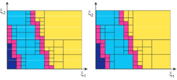
First, we study the quality of the proposed integration technique at the stochas-tic level. In parstochas-ticular, we compare the two proposed recursive procedures for partitioning the stochastic domain Θ (see section 6.2.3). Let K ∈ Th be a given finite element and let CK denote the associated cartesian mesh of Θ, obtained by the isotropic or the anisotropic splitting procedure. We denote by k the maximum order of the partition, which is directly related to the integra-tion precision. Figure 14 presents stochastic domain partiintegra-tions of order k = 4 which are associated with a particular finite element (shown on figure 12). This finite element belongs to the set of possibly cut elements (ec). We ob-serve that the number of stochastic subdomains is lower with the anisotropic splitting (69 versus 88). On this figure, the recursive splitting procedure has stopped for cells C which are not colored in purple. We recall that the recur-sive split stops if all vertices ξ ∈ vertices(C) correspond to the same state SK(ξ) = (sign(φi(ξ)))i∈IK of the finite element K. If we increase the
Let us here recall that ξ1 and ξ2 have not the same range. Axis in Figure 14 have been rescaled for clarity.
ξ2
ξ1 ξ1
ξ2
Fig. 14. Example 1. Stochastic partitions CK of order k = 4 for a particular finite
element K: isotropic splitting (left) and anisotropic splitting (right).
Let NK be the number of subdomains in partition CK. Table 1 shows the mean value of NK over all K ∈ (ec), denoted by µN, for both partition procedures and for different orders of partitions. We note that this number is lower with the anisotropic splitting. We denote by TKthe computational time for creating partition CK and integrating elementary quantities AK and bK. Table 1 also shows the mean time µT over all elements K ∈ (ec). We note that this time is reduced with the anisotropic procedure, especially for high k values. In fact, the computational time of X-SFEM mainly comes from the integration of element quantities for elements in (ec). The computational time TK for K ∈ (ei) and solving the Galerkin system of equations (56) is negligible for this problem (less than 1 second).
partition order k= 0 k = 1 k = 2 k = 3 k = 4 k = 5 µN isotropic 1 4 14 32 69 143 anisotropic 1 4 11 26 54 106 µT isotropic 0.04s 0.11s 0.24s 0.5s 1.1s 2.6s anisotropic 0.04s 0.12s 0.22s 0.46s 1.0s 2.0s Table 1
Example 1. Comparison between the isotropic and anisotropic partitioning proce-dures for different orders k of stochastic partitions: µN is the average number of
stochastic subdomains for elements belonging to (ec) and µT is the corresponding
average CPU times (for creating the stochastic partition and integrating element quantities).
Here, the approximation space contains the exact solution. Then, since X-SFEM is based on a Galerkin projection of the exact physical solution, it leads to the exact solution. However, the obtained approximate solution clearly de-pends on the partition order k (related to the integration precision). Let us denote by σkh,P the associate approximate stress field and by εkthe correspond-ing value of the global error indicator. On figure 15, we show the convergence