Non-linear control of a Narrow Tilting Vehicle

HAL Id: hal-01105300

https://hal.archives-ouvertes.fr/hal-01105300

Submitted on 20 Jan 2015

HAL is a multi-disciplinary open access

archive for the deposit and dissemination of

sci-entific research documents, whether they are

pub-lished or not. The documents may come from

teaching and research institutions in France or

abroad, or from public or private research centers.

L’archive ouverte pluridisciplinaire HAL, est

destinée au dépôt et à la diffusion de documents

scientifiques de niveau recherche, publiés ou non,

émanant des établissements d’enseignement et de

recherche français ou étrangers, des laboratoires

publics ou privés.

Non-linear control of a Narrow Tilting Vehicle

Fabien Claveau, Philippe Chevrel, Lama Mourad

To cite this version:

Fabien Claveau, Philippe Chevrel, Lama Mourad. Non-linear control of a Narrow Tilting Vehicle.

IEEE International Conference on Systems, Man, and Cybernetics (SMC), Oct 2014, San Diego,

United States. pp.2488 - 2494, �10.1109/SMC.2014.6974300�. �hal-01105300�

Non-Linear Control of a Narrow Tilting Vehicle

F. Claveau, Ph. Chevrel, and L. Mourad

IRCCyN, IMT - Ecole des Mines de Nantes La Chantrerie, 4 Rue Alfred Kastler, BP 20722

44307 NANTES, FRANCE fabien.claveau@mines-nantes.fr, philippe.chevrel@mines-nantes.fr

Abstract— Narrow Tilting Vehicles (NTVs) are the

convergence of a car and a motorcycle. They are expected to be the new generation of city cars considering their practical

dimensions and lower energy consumption. But considering their

height to breadth ratio, in order to maintain lateral stability, NTVs should tilt when cornering. Unlike the motorcycle’s case, where the driver tilts the vehicle himself, the tilting of an NTV should be automatic. Two tilting systems are available; Direct and Steering Tilt Control, the combined action of these two systems being certainly the key to improve considerably NTVs dynamic performances. Focusing on the lateral dynamic of NTVs, multivariable control strategies based on linear robust control theory, were already proposed in the literature, assuming decoupling with the longitudinal dynamic. In this paper a 4 DoF model of the main longitudinal and lateral dynamics is considered, and its differential flatness is demonstrated. The three flat outputs have furthermore a particular physical meaning, making possible the design of a simple external control loop complying with the driver demands.

Keywords—Narrow Tilting Vehicle (NTV), Vehicle Dynamics, Flat Systems, Non-Linear State Feedback

I. INTRODUCTION

new generation of cars is currently being studied which will be more practical and efficient in relation to traffic congestion and parking problems in urban areas. These cars are small narrow commuter vehicles, hence saving energy, and are approximately half as wide as a conventional car (less than 1 m). Considering their geometry (approximately 2.5 m long, 1 m wide and 1.5 m high), these cars are characterized by a high centre of gravity, which makes roll stability an issue. To reduce this risk, they may have to lean into corners like two-wheeled vehicles. Some three- and four-wheels NTV projects have already been proposed by several companies. The Ford Gyron is one of the earliest prototypes while General Motors developed the Lean Machine, with a manual lean system controlled by the driver. More recently, Brink Dynamics developed the Carver, a three-wheeled car with a rotating body but a non-tilting rear engine, while the manufacturer Lumeneo proposed the Smera. Two mechanical systems are available to tilt the vehicle [1]-[4]: Direct Tilt Control (DTC) and Steering Tilt Control (STC), see Fig. 1:

- the DTC system is based on a dedicated actuator mounted on the longitudinal axis of the NTV, providing a torque

(Mt) to tilt the vehicle.

- the STC actuator requires a Steer-by-Wire system: the steering angle (δdriv) applied by the driver is modulated by

the STC system (δc) to control the tilt angle using

counter-steering. The tilting strategy is therefore directly inspired by the action of a bicycle or motorcycle rider.

driv δ STC c driv δ δ δ= + Actuator t M Controller DTC ( )R ( )L

Fig. 1. Tilting actuators: DTC (left) and STC (right) systems

STC systems are not well suited for low longitudinal speeds (e.g. less than 8 m.s-1 _{[4]), demanding a large counter-steering}

to tilt the vehicle, which deviates it significantly from its trajectory. In contrast, the STC system may be more efficient than the DTC one at high speed, as a large torque is required by the DTC when entering a bend if the tilting torque occurs a little late. To benefit from the complementary advantages of both systems, several projects have involved the STC and DTC systems working together [4]-[12].

Considering only the DTC actuator, the STC one, or both, several control strategies can be found in the literature; most of them are based on SISO control strategies such as PD / PID controllers as in [3]-[6],[10],[13], tuned potentially thanks to a LQ criterion [3], but assuming a natural decoupling between the roll dynamic of the NTV and the other ones (yaw, longitudinal velocity…). Recent results proposed by Mourad et al. [8], [9] provide multivariable controllers to control the lateral dynamics of SDTC (STC+DTC) vehicles, design thanks to the H2 control theory. A gain-scheduling strategy is

also implemented to make the control law robust to longitudinal velocity variations. In fact, few papers take into consideration the coupling between the longitudinal and the lateral dynamics of these vehicles, and more generally the intrinsic non-linear behavior of NTVs. Considering only the roll dynamic of a DTC vehicle, Piyabongkaran et al. in [3] provide a first non-linear controller (feedback linearization),

and most recent results provided by Roquiero et al. (see e.g. [12]) lead to an interesting non-linear control strategy based on sliding mode, dealing both with the roll and the longitudinal dynamic of a STC narrow vehicle.

Motivated by the fact that non-linear control strategies can potentially reach better solution than the linear ones, it is demonstrated in this paper that a 4 Degrees of Freedom, DoF, non-linear model of a SDTC narrow vehicle has flatness properties, and more precisely it can be linearized thanks to a static state feedback [14]-[16]. Such non-linear systems are quite interesting, as once linearized, one can implement linear control strategy on the new input / output mapping. Furthermore, flat outputs can be found, with interesting physical meanings (Huygens oscillation center [16],[17]), making easier the design of the external tracking loop. This work can be seen as a generalization of results proposed by Fuchshumer et al. [18] demonstrating that the non-linear longitudinal – lateral so-called bicycle model is flat.

The paper is organized as follows: Section 2 presents the SDTC NTV 4 DoF model and the associated assumptions. Section 3 makes some reminders on the definition and the properties of flat systems, used in Section 4 to demonstrate the flatness property of the NTV model. The linearizing state feedback is defined in Section 5, as well as the external loop based on a simple trajectory generator and PI/PD controllers. Results obtained in simulation are shown in Section 6. The conclusion and perspectives are presented in Section 7.

II. 4DOF NON-LINEAR NTV MODEL A. 4 DoF Model of the Longitudinal-Lateral Dynamics

Several NTV models were proposed in the literature; see e.g. [4],[10]-[13],[19] or [8],[9] for a short survey of the different models. The University of Minnesota has proposed several non-linear and linear models [1],[3],[5],[6], in particular a 3 DoF non-linear model to study the lateral dynamics of NTVs. lr F sr F r α f α β δ lf F sf F y r v ψ x X Y G v x v y θ h 2 θ h g θ G z ' z ' y t M motion direction y

Fig. 2. Four DoF of the tilting vehicle: top view (left) and rear view (right) In this paper a 4 DoF model is proposed, based on the non-linear 3 DoF model of the lateral dynamics of a NTV [1], considering the longitudinal speed of the vehicle as a parameter of the model, and the so-called 3 DoF “bicycle” model modeling the lateral and longitudinal dynamics of the vehicle. As depicted in Fig. 2, the 4 DoF are the longitudinal and lateral position (x,y) of the vehicle, the tilt angle θ, and the yaw angle

ψ. In the absolute reference (XYZ), the reference (xyz) is attached to the centre of gravity G of the vehicle, with (xy) the horizontal plane, (x) being parallel with the longitudinal axis of the vehicle. The reference (x’y’z’) is also attached to the centre of gravity, but leans with the chassis, i.e. (x) and (x’) are the same. The reference (xvyvzv) is also linked to G, but the axis (xv)

is collinear to the longitudinal speed of the vehicle v, and (zv) is

collinear to (Z).

The 4 DoF model was build under the following assumptions: 1- the vehicle is considered a mass point at its centre of gravity; 2- vertical reaction forces on the right and left wheels are considered identical; 3- gyroscopic effects due to the rotation of the wheels and road bank angle are neglected; 4- many mechanical parts that would have an impact on the vehicle’s dynamics are not represented (e.g. dampers). Nevertheless, this simplified model can still be used for control, as long as the control law has some robustness. All this leads to the non-linear model x₌ f x u

( )

, , with the state vector x_{= ⎣}⎡v β ψ θ θ⎤_⎦T, and the control input signals

[

]

T

l t

u_{= δ} F M

2

2

1_{( sin( ) cos( ) sin( ) cos( ))}

( cos sin )sin 1 _{( cos( ) sin( ) cos( ) sin( ))}

1_{( cos sin ) cos}

( cos sin ) sf lf sr lr sf lf sr lr f _r sf lf s v F F F F m h h r F F F F mv h h v l l r F F F J J β δ β − δ β β θ θ θ θ β β β δ β δ β β θ θ θ θ β ψ δ δ − = − + + + − − = − + − − − + − − − = = + 2 2 2 2

( cos sin ( cos sin ) cos sin ) ( sin ) r sf lf sr s t x mh F F F h hF M I mh θ = θ θ θ θ δ δ θ θ θ θ ⎧ ⎪ ⎪ ⎪ ⎪ ⎪ ⎪ ⎪ ⎪ ⎪ ⎨ ⎪ ⎪ ⎪ ⎪ ⎪ ⎪ ⎪ _{− − + + + +} ⎪ = ⎪ ₊ ⎩ (1)

All the signals and parameters are defined in Table 1.

lr l

F =γF, F_lf = −

(

1 γ

)

F_l, γ∈

[ ]

0,1 meaning that the motor or braking force can be supplied to the front and the rear wheel with a given transmission ratio (all-wheel driven vehicle). γ is assumed to be a constant value in this paper, to fit with the reality of NTVs (most being characterized by the ratio γ = 1). The other control inputs are the steering angle of the front wheel δ and the tilting torque Mt, i.e. the NTV is equipped of

both a DTC and STC system.

B. Rear and Front Lateral Tire Forces

Several models of the lateral tire forces Fsf and Fsr can be

found in the literature, see e.g. [20]. One common assumption is that these lateral tire forces can be expressed as functions of the side-slip angles αf and αr of the wheels:

1 sin 1 sin tan , tan cos cos f _r f r v l v l v v β ψ β ψ α δ α β β − ⎛ + ⎞ − ⎛ − ⎞ = − ⎜ ⎟ = − ⎜ ⎟ ⎝ ⎠ ⎝ ⎠ (2)

and also of the tilt angle _θ of the vehicle through the camber stiffness of the tires. Considering the small angle approximation tan φ≈φ, the lateral tire forces models are,

(

)

(

)

sin , , , 2 2 , cos sin , , 2 2 . cos f sf f f r sr r r v l F v r C v v l F v r C v β ψ δ β δ λ θ β β ψ β _β λ θ ⎧ ⎛ + ⎞ = − + ⎪ ⎜ ⎟ ⎪ ⎝ ⎠ ⎨ − ⎛ ⎞ ⎪ _{= +} ⎜ ⎟ ⎪ _{⎝ ⎠} ⎩ (3)

Notice however that, as suggested in [18], in the flatness analysis of the non-linear model (1)-(3), the detailed expression of the lateral tire forces Fsf(δ,v,β,r) and Fsr(v,β,r)

are not necessary. Assuming them as smooth functions is a sufficient technical condition to make easier the mathematical manipulations.

Table 1. Parameters of The 3 DoF Model: See [1],[8] For Numerical Values

v longitudinal speed of the _vehicle g gravitational constant β side-slip deviation angle m total mass

, r

ψ =ψ _{yaw angle and speed h} position of the center of gravity G on the z’ axis ,

θ θ tilt angle and speed Iz vehicle yaw moment of _inertia

Mt tilting torque provided by the _{DTC actuator} Ix vehicle roll moment of _inertia

δ steering angle of the front _wheels lf distance from center of _{gravity to front axle}

Fl global longitudinal force lr distance from center of _{gravity to rear axle}

αf, αr front and rear tire side-slip _angle Cf, Cr front and rear cornering _stiffness

Flf, Flr front and rear longitudinal _force λf, λr front and rear camber _stiffness

Fsf, Fsr front and rear lateral force

C. Control Objectives in Terms of Lateral Stability of NTVs As said in the introduction, the objective is to ensure the lateral stability of the NTV faced with lateral acceleration when cornering, by tilting its chassis thanks to the DTC and STC systems. In particular, the lateral acceleration at the center of gravity G is of importance.

Definition 1: Perceived acceleration aper

aper denotes the resultant acceleration at the center of gravity G, along the axis (y’) (cf. Fig. 2), i.e. perpendicular to the chassis of the vehicle. It is linked to other variables by:

(

)

cos sin cos sin

per lat

a =a θ+hθ−g θ= y V+ ψ θ+hθ−g θ(4)

The terminology "perceived" (or measured) acceleration was introduced in [1]. This would be the acceleration measured by an accelerometer positioned at the center of gravity whose lateral axis is in the lateral vehicle direction,

and also the lateral acceleration perceived by the driver in the cabin of the vehicle, impacting the comfort. Fundamentally, the lateral stability of the NTV is ensured if aper = 0. To reach

this objective, the literature classically reformulates the lateral control problem as an angular position tracking problem, regulating the tilting angle θ around the reference angle θref,

estimated on line by inverting equation (4) (with more or fewer approximations) [3]-[7],[11]-[13]. There are pros and cons for such control strategy as discussed in [9], compared to the direct regulation of aper as proposed by the authors e.g. in

[8],[9]. As it will be detailed in Section 5, the tilt angle control strategy will be applied in this paper, to be consistent with the physical meaning of the chosen flat outputs. Concretely, our fundamental control objective is defined by the following equation 1 cos tan 0 ref rv _g β θ θ_{− = −}θ − ⎛_⎜ ⎞_⎟= ⎝ ⎠ . (5)

The other control objectives will be to ensure the trajectory planning and regulation to satisfy the driver’s desires, express through the throttle/brake pedal, traduced as a desired longitudinal traction force Fl-driv, and the steering wheel angle δdriv. A first simple solution is also provided in Section 5.

D. Available Measurements

Practically, tilting cars generally include a tilt angle sensor and an Inertial Measurement Unit (IMU), which provide the state values v, θ, θ , ψ and aper. Lastly, the steering angle

δ and its derivative are assumed to be can be measured, and the side-slip angle β available through an estimator (e.g. [21]).

III. FLATNESS PROPERTY AND STATIC STATE FEEDBACK LINEARIZATION

A. Flatness property

The main objective in this paper is to demonstrate, in the same spirit as in [18], that the longitudinal / lateral 4 DoF model of a NTV equipped with a SDTC system can be linearized by a static non-linear state feedback. To prove such a result, 3 flat outputs associated to the 3 control inputs, will be first exhibited. To begin with, some reminders about the flatness property are proposed hereafter.

Definition 1: Flat system [15]

Consider a non-linear system x= f x u

( )

, , _x∈ n_{, u∈} m_.

Such system is said to be a “flat system”, if and only if one can find: - an output vector _y∈ m_, - r∈ and functions o 1 : n ( m r) m R R + R Π × → , with rank m, o _Ω: (_Rm r) _→Rn_{, with rank n,}

o _{Ξ: (R}m r₎+1_→Rm_{, with rank m,}

such as one can write:

( ) 1 2 ( 1) ( ) ( , ,..., ) ( , , ,..., ), ( , ,..., ), ( , ,..., ). r m r r y y y y x u u u x y y y − u y y y ⎧ = = Π ⎪ ⎨ = Ω = Ξ ⎪⎩ (6)

In fact, a system verifying the flatness property is such that all its state and input signals can be expressed as functions of some specific output signals hence named flat outputs. In other words, these outputs “sum up” all the dynamic characteristics of the system.

Definition 2: Relative degree

Consider a non-linear system

( )

( )

1 1

( )

( )

( )

, , , , m m x f x u x f x u y h x y h x y h x ⎧ = ⎧ = ⎪ ⎪ ⇔ ⎨ ⎨ = = = ⎪ ⎪ ⎩ ⎩ … (7)

with _x∈ n_{, u∈} m_{, and m scalar outputs y}

i. The smallest integer r_i∈ such as yi( )ri 0

u

∂ _≠

∂ is the relative degree of

the output yi.

Property 1: Flat outputs

Consider the non-linear system (7). If one can find a change of coordinates z= Φ

( )

x such that:

- Φ is a diffeomorphism, and the new state

( )

. _z∈ n _is

composed of the m outputs yi and their derivatives until the (ri - 1) degree, i.e.

(1 1) ( 1) 1 1 1 m T r r m m m z_{= ⎣}⎡y y y − y y y − ⎤_{⎦ , (8)}

- the decoupling matrix M is full rank, rank(M) = m,

( ) 1 , 1 j r j i i m j m y M _u ≤ ≤ ≤ ≤ ⎡_∂ ⎤ ⎢ ⎥ = _∂ ⎢ ⎥ ⎣ ⎦ (9)

then ouputs yi are flat outputs of the system.

B. Input / State Feedback Linearization Property 2: Exact static state feedback

If a non-linear system as (7) is flat, with furthermore the relative degrees of the several flat outputs yi such as

1 m i i r n = =

∑

,

then system (7) is exact input / state linearizable via static state feedback, i.e. one can find a static non-linear state

feedback with the new inputs _ω∈ m_{, defined as the solution}

of ( )

_{( )}

( )

_{( )}

( )

_{( )}

1 2 1 1 2 2 , , , m r r r m m y x u y x u y x u ω ω ω ⎧ ₌ ⎪ = ⎪ ⎨ ⎪ ⎪ = ⎩ (10)

such that the closed-loop is equivalent to the linear time invariant system (11) based on m chains of integrators

1 2 1 1 1 2 2 1 1 2 1 1 1 1 1 1 2 2 1 1 1 1 1 1 2 1 1 0 0 0 0 0 0 0 0 0 0 0 0 m m m m z r r r r z r r r z r r z m m r z r r z z r r r z m _m r z A B B A z z B A C y C z y C ω × × × × × × × × × × × × ⎧ ⎡ ⎤ ⎡ ⎤ ⎪ ⎢ ⎥ ⎢ ⎥ ⎪ ₌⎢ ⎥ ₊⎢ ⎥ ⎪ ⎢ ⎥ ⎢ ⎥ ⎪ ⎢ ⎥ ⎢ ⎥ ⎪ ⎢ ⎥ ⎢ ⎥ ⎪ ⎣ ⎦ ⎣ ⎦ ⎨ ⎡ ⎤ ⎪ ⎢ ⎥ ⎡ ⎤ ⎪ ⎢ ⎥ ⎢ ⎥ ⎪ _{= ⎢} ⎥ ⎢ ⎥ ⎪ ⎢ ⎥ ⎢ ⎥ ⎪⎣ ⎦ ⎢ ⎥ ⎪ _{⎣ ⎦} ⎩ (11) with matrices i z A , i z B , i z C of dimensions r r_i× , _i r_i× , 11 × , ri

( )

( )

0 1 0 0 1 0 0 i z A ⎡ ⎤ ⎢ ⎥ ⎢ ⎥ = ⎢ ⎥ ⎢ ⎥ ⎢ ⎥ ⎣ ⎦ , 0 0 1 i z B ⎡ ⎤ ⎢ ⎥ ⎢ ⎥ = ⎢ ⎥ ⎢ ⎥ ⎣ ⎦ , i

[

1 0 0

]

z C = .

IV. FLATNESS PROPERTY OF THE NTV MODEL Considering the previous definitions and properties, some flat outputs are proposed in this section, demonstrating that the 4 DoF model of NTVs in (1) can be linearized, under few assumptions, thanks to a static state feedback.

A. Main Results Proposition 1

Let’s consider that the lateral tire forces Fsf(δ,v,β,r) and Fsr(v,β,r) are arbitrary smooth functions. Let’s define the

smooth function

(

)

(

)

(

)

2 ( , , ) ( , , , , cos , , sin ) cos f r r sr sr f f v sr f l l J T v r v F v r F v r ml ml J v F v r v ml β β β β β β β β + = ∂ + ∂ + ∂ − (12)

with the notation ∂_ωF=∂F_∂ω. Then under the conditions T(v,β,r) ≠ 0, v ≠ 0, the non-linear system (1) is differentially flat. Furthermore, this system is exact input / state linearizable via a static feedback. In particular, the 3 outputs (13) are available flat outputs with relative degrees (1,2,2).

( )

( )

( )

1 1 2 2 3 3 cos sin cos f y h x v J y y h x v h ml y h x β β θ θ θ ⎧ _{= =} ⎪ ⎪ = = − + ⎨ ⎪ ⎪ _{= =} ⎩ (13)

Proof: see [8]-chap.6 for the detailed proof. At first, the relative degree of the 3 outputs y1, y2, y3 can be easily verified

by computing derivatives

₍

y y y₁, ₂, ₃

₎

. Let’s then consider the coordinates transformation

( )

1 1 2 2 3 2 4 ₃ 3 5 cos sin cos cos f f r sr f v z _y J v r h ml z y l l y z x z z _{F vr} ml y z y z β β θ θ β θ θ ⎡ ⎤ ⎢ ⎥ ⎡ ⎤ ⎡ ⎤ ⎢ ⎥ ⎢ ⎥ _{⎢ ⎥ ⎢} − + _⎥ ⎢ ⎥ ⎢ ⎥ ⎢ ⎥ ⎢ ⎥ + ⎢ ⎥ ⎢ ⎥ = Φ ⇔ =⎢ ⎥= = ₋ ⎢ ⎥ ⎢ ⎥ ⎢ ⎥ ⎢ ⎥ ⎢ ⎥ ⎢ ⎥ ⎢ ⎥ ⎢ ⎥ ⎢ ⎥ ⎣ ⎦ ⎢ ⎥ ⎢ ⎥ ⎣ ⎦ _{⎢ ⎥} ⎣ ⎦ . (14)

( )

x

Φ is a diffeomorphism as long as det(J) ≠ 0,

1 , 1

( )

_i i n j j n

x

J

_x

≤ ≤ ≤ ≤

⎡

_∂Φ

⎤

= ⎢

_⎣

_∂

⎥

_⎦

. This is equivalent to the condition

T(v,_β,r) ≠ 0. Moreover, the decoupling matrix

1 1 1 2 2 2 3 3 3 l t l t l t F F F y y y M y y y y y y δ Μ δ Μ δ Μ ⎛_{∂ ∂ ∂} ⎞ ⎜ ⎟ = ∂⎜ ∂ ∂ ⎟ ⎜ ⎟ ⎜_{∂ ∂ ∂} ⎟ ⎝ ⎠ (15)

remains of full rank for T(v,β,r) ≠ 0 and v ≠ 0. This proves the flatness of y (13) (see Property 1). … B. Physical Meaning of the Proposed Flat Outputs

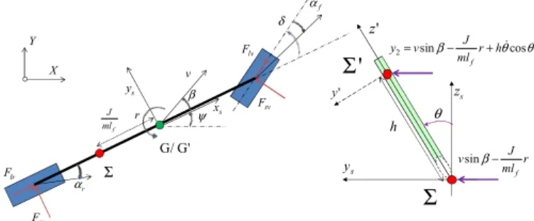
The chosen flat outputs in (13) have some physical meaning of interest to build the external tracking loop. Defining the point G’, projection on the vehicle’s longitudinal axis of the center of gravity G along the axis (z’), we define in Fig. 3 the new reference (xsyszs) linked to G’: it is the translation of reference

(xyz) in Fig. 2 from G to G’. Let’s define the specific points

(

J lm/ _f,0,0

)

Σ − and ∑'

(

−J ml h/ _f, sin , cos_θ h _θ

)

in this

reference (xsyszs). Considering this new reference and the two specific points Σ and Σ’, one can observe that: y1 is the

longitudinal speed of any point located on the vehicle’s longitudinal axis (xs), y2 is the lateral speed of Σ’ in (xsyszs), y3

is the tilting angle of the vehicle. Remark: Huyghens center of oscillation

As in [18], the specific point Σ’ can be linked to the

Huyghens center of oscillation, define in a general manner for Lagrangian systems underactuated by one control, such as the PVTOL position control in [17].

lr F sr F r α f α β δ lv F sv F s y r v ψ xs X Y G/ G' Σ f J ml θ 2 sin cos f J y v r h ml β − θ θ = + s z ' z ' y s y

Σ

sin f J v r ml β− h

'

Σ

Fig. 3. Top view (left) and Front view (right) of the vehicle: definition of the point Σ’

(

−J ml h/ _f, sin , cosθ h θ

)

in reference (xsyszs)

V. CONTROL DESIGN A. Design of the static state linearizing feedback

According to Property 2, the 4 DoF NTV model controlled

by the ad hoc non-linear feedback depicted in Fig. 4 is

equivalent to the linear one defined by equations (10),(11), under restriction (12). The analytic expression not presented here by lack of place, is available however in [8]-prop. 6.3.

state feedback t M δ l F x ⇔ 1 y 3 y 2 y ( , ) x=f x u 1 ω 2 ω 3 ω 1 y 3 y 2 y ∫ ∫ ∫ ∫ ∫ 1 ω 2 ω 3 ω

Fig. 4. Equivalent closed-loop system

B. Design of the tracking controller and trajectory generation

Finally, we have to regulate y (see equation (13)) around

some trajectories that 1/ ensure the lateral stability of the vehicle, 2/ interpret and satisfy the driver’s desires. His demand is made through the steering wheel angle and the throttle / break pedal. This is still partly an open research topic. δdriv the steering wheel angle reference, and Fl-driv the required longitudinal force are considered here as the new input left at the disposal of the driver. Fig. 5 depicts the solution proposed at this first stage, involving the three reference signals: 1 0 0 2 0 0 1 3 cos cos sin sin cos tan t d l driv

x driv driv driv

t

d l driv

y driv driv driv

d ref F y v v v m F y v v v m rv y g δ δ δ δ β θ − − − − − ⎧ ⎛ ⎞ ⎪ _{= = =}⎜ ₊ ⎟ ⎜ ⎟ ⎪ _{⎝ ⎠} ⎪ ⎪ _{⎛ ⎞} ⎪ _{⎜ ⎟} = = = + ⎨ _{⎜ ⎟} ⎪ _{⎝ ⎠} ⎪ ⎛ ⎞ ⎪ _{= =} ⎜ ⎟ ⎪ _{⎝ ⎠} ⎪⎩

∫

∫

(16)

The two first reference signals make possible the control of the lateral and longitudinal speeds. The third is the tilting

reference θref, classically computed as proposed in the

3 d y 2 d y 1 d y Génération de la trajectoire 1 y ( , )x y 2 y 3 y l cond F₋ 1/ m _∫ cos sin w1 Système _{y 3} 1 PD PD2 cond δ 3 PD PIδ ( ) ref f x θ = 1 y 2 y δ + + + + + − − − + − 1 ω 2 ω 3 ω Linearized system Trajectory generation Fl-driv δdriv

Fig. 5. Trajectory generation tracking applied to each decoupled wi→yi. Three PD controllers are implemented to drive the error signals e_i = −y_i y_id, i = 1,2,3. A PI is also used to generate the control signal ω2, to control the error signal eδ = δ - δdriv. Finally, it leads to,

(

)

(

)

2 2 2 , 1,3 P D i i i i I P D P i K K s e i K K K s e K e s δ δ δ ω ω ⎧ _{= + =} ⎪⎪ ⎨ ⎛ ⎞ = + + + ⎪ ⎜_⎜ ⎟_⎟ ⎪ ⎝ ⎠ ⎩ (17) VI. RESULTS

The performances of the proposed control strategy are now evaluated by simulating the non-linear model (1). The scenario is defined as follows: the driver requires a constant acceleration (Fl-driv assumed to be constant), and the steering wheel angle δdriv (see Fig. 6) entails a first bend followed by a circular trajectory (medium sized roundabout). This trajectory is quite difficult compared to the ones proposed e.g. in [3] or [7]. The PDs and PI controllers considered were tuned to:

- PD1: K1P =2, 0.2KiD= , PD3: K3P =0.6, K3D=1.3,

- PD2: K2P =3.5, K2D=5, PIδ : 40KδP = , 0.2KδI = .

The simulation results are compared with the ones obtained with the LPV controller proposed in [9], designed by solving

a H2 control problem based on the linearized model of the

lateral dynamic of the NTV, considering as controlled output

the lateral acceleration aper, and made robust to the

longitudinal velocity variation thanks to a gain-scheduling solution. Fig. 6 firstly shows that the gap between the desired

steering angle _δdriv and the one applied by the non-linear

controller _{δ through} the STC system is not intrusive.

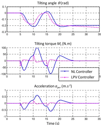
Considering the traction force, Fl is identical to the desired one Fl-driv in a straight trajectory, but is reduced in bend, so as to ensure a better trajectory tracking. Even if it can be seen as a driving assistance, such behavior can be disturbing for the driver and should be studied in more depth in the future. However, results in Fig. 7 and Fig. 8 show that the proposed non-linear control strategy associated to the rudimentary trajectory generation system (16) ensures the lateral stability of the vehicle: in particular, the perceived acceleration aper

reaches acceptable values (max. 0.6 m/s²), compared to most

of the results in the literature. The LPV controller still reaches

better performances, with a tilting torque Mt divided by a

factor 2 and a lateral acceleration aper 3 times smaller.

However we are convinced that a more sophisticated external loop should improve the performances.

5 10 15 20 25 30 35 0 5 10 Temps (sec) F_l-véhicule F_l-cond 0 5 10 15 20 25 30 35 6 6.5 7 7.5 Vitesse longitudinale temps (s) Contrôleur NL Contrôleur LPV Longitudinal velocity v (m.s-1₎ NL Controller LPV Controller 5 10 15 20 25 30 35 -0.1 -0.05 0 δ δ_roues δ_cond Time (s) Traction force Fl (N)

Steering angle δ(rad)

δdriv

Fl Fl-driv

Fig. 6. Longitudinal velocity of the NTV (Non-Linear and LPV solution), steering, desired steering angle _δdriv and traction force Fl-driv, and the ones

calculated by the complete non-linear controller, _{δ , F}l.

0 5 10 15 20 25 30 35 -0.3 -0.2 -0.1 0 0.1

Angle d′ inclinaison θ (rad)

0 5 10 15 20 25 30 35 -100 -50 0 50 100 Signal de Commande M_t 0 5 10 15 20 25 30 35 -1 -0.5 0 0.5 1

Accélération perçue a_per

temps (s)

Contrôleur NL Contrôleur LPV

NL Controller LPV Controller Tilting angle θ(rad)

Tilting torque Mt(N.m)

Acceleration a_per(m.s-2₎

Time (s)

Fig. 7. Tilting angle, tilting torque of the DTC system, and lateral perceived acceleration obtained by the non-linear (NL) and the LPV controller.

0 10 20 30 40 50 60 70 -80 -70 -60 -50 -40 -30 -20 -10 0 10 j x y Contrôleur NL Contrôleur LPV NL Controller LPV Controller

Fig. 8. NTV Trajectory considering the non-linear (NL) controller and the LPV one.

VII. CONCLUSION AND PERSPECTIVES

Based on a 4 DoF model of a Narrow Tilting Vehicle equipped both of a DTC and STC system, inspired from the well-known bicycle model and the 3 DoF model of the lateral dynamic of NTVs [1], we showed that NTVs verify the differential flatness property. Furthermore, they present some interesting characteristics. First, based on few assumptions on the tire forces model, the longitudinal-lateral dynamics of NTV can be linearized thanks to a static state feedback. Secondly, three flat outputs with a concrete physical meaning associated to the Huyghens oscillation center, can be defined. To validate the proposed linearizing feedback, a first control strategy based on a rudimentary trajectory generation system and PD/PI control loops was also proposed. It has been demonstrated that such simple external loops already reach quite satisfactory performance.

These first results call for some motivating perspectives: a classic state feedback was design here, leading to three decoupled integrator chains. Such strategy has the weakness to “erase” the original dynamics of the system. We believe that methods inspired by [22] will bring more robustness; a linearizing feedback leading to a closed-loop system sharing structural properties with the tangent linear models of the original system. On this basis, we then plan to make use of the optimal control strategy proposed in [9] for the external loop synthesis, thus bypassing the gain-scheduling design step while getting an improved performance.

ACKNOWLEDGMENT

The authors wish to thank C. H. Moog for the fruitful discussions we had together.

REFERENCES

[1] R. Rajamani, J. Gohl, L. Alexander, and P. Starr, “Dynamics of narrow tilting vehicles”. Math. and Comp. Model. of Dyn. Sys., vol. 9, n°2, 2003, pp. 209-231.

[2] R. Rajamani, Vehicle Dynamics and Control. Springer, US, 2006, Chapter 2.

[3] D. Piyabongkarn, T. Keviczky, and R. Rajamani; ‘‘Active Direct Tilt Control for stability enhancement of a narrow commuter vehicle,’’

Intern. Journ. of Auto. Tech., vol. 5, n°2, 2004, pp. 77-88.

[4] S.G. So and D. Karnopp, ‘‘Active dual mode tilt control for narrow

ground vehicles,’’ Veh. Syst. Dyn., vol. 27, 1997, pp. 19-36.

[5] S. Kidane, L. Alexander, R. Rajamani, P. Starr, and M. Donath, “Road bank angle considerations in modeling and tilt stability controller design for narrow commuter vehicles,” in Proc. IEEE Amer.. Contr. Conf., Minneapolis, USA, 2006.

[6] S. Kidane, L. Alexander, R. Rajamani, P. Starr, and M. Donath “A fundamental investigation of tilt control systems for narrow commuter vehicles,” Veh. Syst. Dyn., vol. 46, 2008, pp. 295-322.

[7] R. Hibbard and D. Karnopp, “Twenty first century transportation system solutions- A new type of small, relatively tall and narrow active tilting commuter vehicle,” Veh. Syst. Dyn., vol. 25, 1996, pp. 321-347. [8] L. Mourad, “Active lateral acceleration control of a narrow tilting

vehicle,” Ph.D. Dissertation, Ecole des Mines de Nantes, Nantes, 2012 (in French). http://hal.archives-ouvertes.fr/tel-00787310/

[9] L. Mourad, F. Claveau, Ph. Chevrel, “Direct and steering tilt robust control of narrow vehicles,” IEEE Trans. Intel. Transp., Sys., accepted, in press, T-ITS-13-05-0237, DOI : 10.1109/TITS.2013.2295684

[10] J. Roberston, J. Darling, and A. Plummer, “Path following performance of narrow tilting vehicles equipped with active steering,” in Proc. 11th

Conf. on Eng. Sys. Design and Ana., Nantes, France, 2012.

[11] J.H. Berote, “Dynamics and control of a tilting three wheeled vehicle,” Ph.D. Dissertation, University of Bath, UK, 2010.

[12] N. Roquiero, G. d.F. Marcelo, and F.C. Enric, “Sliding mode controller and flatness based set-point generator for a three wheeled narrow vehicle,” in Proc. 18th IFAC World Congress, Milano, Italy, 2011. [13] J.C. Chiou and C.L. Chen, “Modeling and verification of a diamond

shape narrow tilting vehicle,” IEEE/ASME Trans. on Mech., vol. 13, n°6, pp. 678-691, 2008.

[14] G. Conte, C. H. Moog, and A.M. Perdon, Algebraic methods for

nonlinear control system. 2nd _{ed., London: Springer, 2007.}

[15] M. Fliess, J. Lévine, and P. Rouchon, “Flatness and defect of nonlinear systems: introductory theory and examples,” Intern. Journ. of Contr.,

vol. 61, n°6, pp. 1327-1361, 1995.

[16] P. Martin, R.M. Murray, qnd P. Rouchon, Flat systems, equivalence and trajectory generation, CDS Technical Report, CDS 2003-008, 2003. [17] P. Martin, S. Devasia, and B. Paden, “A different look at output

tracking: control of a VTOL aircraft,” Automatica, vol. 32, n°1, pp.

101-107, 1996.

[18] S. Fuchshumer, K. Schlacher, and T. Rittenschober, “Nonlinear vehicle dynamics control – a flatness based approach,” in Proc. IEEE Conf. on

Decis. and Contr., Sevilla, Spain, 2005.

[19] S. Maakaroun, Ph. Chevrel, M. Gautier, and W. Khalil, “Modeling and Simulation of a Two wheeled vehicle with suspensions by using Robotic Formalism,” in Proc. 18th IFAC World Congress, Milano, Italy, 2011. [20] E. Bakker, H. Pacejka, and L. Lidner, “A new tire model with an

application in vehicle dynamics studies,” SAE Paper N°890087, pp.

101-113, 1989.

[21] J. Stephant, A. Charara and D. Meizel, “Virtual sensor, application to vehicle sideslip angle and transversal forces”, IEEE Trans. Industrial

Electronics, vol. 51, no. 2, pp. 278-289, 2004.

[22] A. L.D. Franco, H. Bourlès, and E. R.D. Pieri, “Robust feedback linearization without full state information,” in Proc. IFAC Symp. Sys.