HAL Id: tel-00659362
https://tel.archives-ouvertes.fr/tel-00659362
Submitted on 12 Jan 2012HAL is a multi-disciplinary open access archive for the deposit and dissemination of sci-entific research documents, whether they are pub-lished or not. The documents may come from teaching and research institutions in France or abroad, or from public or private research centers.
L’archive ouverte pluridisciplinaire HAL, est destinée au dépôt et à la diffusion de documents scientifiques de niveau recherche, publiés ou non, émanant des établissements d’enseignement et de recherche français ou étrangers, des laboratoires publics ou privés.
Vehicles
Mathieu Balesdent
To cite this version:
Mathieu Balesdent. Multidisciplinary Design Optimization of Launch Vehicles. Optimization and Control [math.OC]. Ecole Centrale de Nantes (ECN), 2011. English. �tel-00659362�
ARCHITECTURE
École Centrale de Nantes
Année 2011
Thèse de Doctorat
Spécialité : Génie Mécanique
présentée et soutenue publiquement parMathieu BALESDENT
le 3 novembre 2011
à
l’Office National d’Etudes et de Recherches Aérospatiales
OPTIMISATION MULTIDISCIPLINAIRE DE
LANCEURS
(Multidisciplinary Design Optimization of Launch Vehicles)
JURY
Président :
Jean-Antoine Désidéri Directeur de Recherche, INRIA Rapporteurs :
David Bassir Docteur, HDR, Université de Technologie de Belfort-Montbéliard
Attaché pour la Science et la Technologie, Ministère des Affaires Etrangères Patrick Siarry Professeur, Université Paris-Est Créteil Val-de-Marne
Examinateurs :
Philippe Dépincé Professeur, Ecole Centrale de Nantes Michèle Lavagna Associate Professor, Politecnico di Milano
Rodolphe Le Riche Docteur, HDR, CNRS - Ecole des Mines de Saint-Etienne Invités :
Nicolas Bérend Ingénieur, Onera Julien Laurent-Varin Docteur, CNES
Directeur de thèse : Philippe DÉPINCÉ Encadrant Onera : Nicolas BÉREND
Laboratoires : Office National d’Etudes et de Recherches Aérospatiales
Institut de Recherche en Communications et Cybernétique de Nantes
This work has been realized in the Onera’s System Design and Performance Evaluation Department, in collaboration with the CNES Launchers Directorate and the team Systems
Engineering Products, Performance and Perceptions of IRCCyN. I would like to thank the
director of DCPS, Dr. Donath, for giving me the opportunity to achieve this thesis at Onera. I would like to thank Dr. Désidéri, who did me the honour of chairing my PhD commit-tee. I express my gratitude to Dr. Bassir and Prof. Siarry for reviewing this PhD thesis. I also thank Dr. Laurent-Varin, Prof. Lavagna and Dr. Le Riche for accepting to be part of my PhD committee.
I would like to acknowledge Prof. Dépincé for agreeing to be my advisor during these three years. I would like to express my thankfulness to my Onera supervisor, M. Bérend for his comments, suggestions, edits, and advices during the thesis.
I would like to thank my CNES supervisor, M. Oswald. I thank also M. Amouroux for his help in the elaboration of the launch vehicle disciplinary models.
I owe a great amount of thanks to the people whom I’ve been working with every day at the Onera’s DCPS. Especially, I thank Dr. Piet-Lahanier for her numerous advices all along the thesis.
I would also like to thank the Onera PhD students (Dalal, Ariane, Rata, Walid, Julien, Joseph, François, Yohan and Damien) who have provided the most exciting working envi-ronment. Special thanks go to my office mate, Rudy, qui quæsivit rerum causas, for those numerous happy hours spent during the thesis.
Last but not least, I would like to thank my parents, who believed in me and always encouraged me. Finally, I would especially like to thank my fiancée Sophie, for all her love and for her understanding when I spent my time working on this thesis. I appreciate her support and her sacrifices very much during this endeavor.
Hercules Furens
Nomenclature
13
Acronyms
15
Introduction
17
I
Panorama of Multidisciplinary Design Optimization methods
used in Launch Vehicle Design
21
1 Generalities about Multidisciplinary Design Optimization 23
1.1 Introduction . . . 23
1.2 Mathematical formulation of the general MDO problem . . . 24
1.2.1 Problem formulation . . . 25 1.2.2 Types of variables . . . 25 1.2.3 Types of constraints . . . 26 1.2.4 Types of functions . . . 26 1.2.5 Disciplinary equations . . . 26 1.2.6 Coupling . . . 27 1.2.7 Multidisciplinary analysis . . . 28
1.3 Feasibility concepts in MDO . . . 28
1.3.1 Individual disciplinary feasibility . . . 28
1.3.2 Multidisciplinary feasibility . . . 29
1.4 Description of the Launch Vehicle Design problem . . . 29
1.4.1 Disciplines and variables . . . 29
1.4.2 Constraints . . . 30
1.4.3 Objective functions . . . 30
1.4.4 Specificities of the Launch Vehicle Design problem . . . 30
1.5 Conclusion . . . 31
2 Classical MDO methods 33 2.1 Introduction . . . 33
2.2 Single level methods . . . 34
2.2.3 All At Once . . . 38
2.3 Qualitative comparison of the single level methods . . . 39
2.4 Multi level methods . . . 40
2.4.1 Collaborative Optimization . . . 40
2.4.2 Modified Collaboration Optimization . . . 42
2.4.3 Concurrent SubSpace Optimization . . . 44
2.4.4 Bi-Level Integrated Systems Synthesis . . . 46
2.4.5 Analytical Target Cascading . . . 49
2.4.6 Other multi level methods . . . 51
2.5 Conclusion . . . 52
3 Optimization algorithms and optimal control techniques 53 3.1 Introduction . . . 53
3.2 Optimization algorithms used in MDO . . . 54
3.2.1 Gradient-based algorithms . . . 54
3.2.2 Gradient-free algorithms . . . 55
3.3 Optimal control . . . 62
3.3.1 Direct methods . . . 64
3.3.2 Indirect methods . . . 65
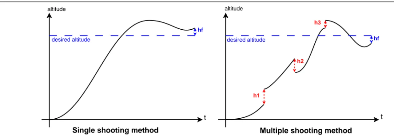
3.3.3 Single vs multiple shooting methods . . . . 66
3.3.4 Collocation methods . . . 68
3.3.5 Dynamic Programming . . . 69
3.4 Conclusion . . . 69
4 Analysis of the MDO method application in the Launch Vehicle Design 71 4.1 Introduction . . . 71
4.2 Different study cases and optimization criteria . . . 72
4.2.1 MDO methods and optimization algorithms . . . 72
4.2.2 Optimization criteria and different study cases . . . 73
4.3 Trajectory handling . . . 73
4.4 Comparison of the main MDO methods in a common application case . . . . 74
4.4.1 Presentation of the optimization problem . . . 74
4.4.2 Comparison of AAO, MDF and CO . . . 74
4.4.3 Comparison of FPI, AAO, BLISS2000 and MCO . . . 75
4.5 Comparative synthesis of the main MDO methods . . . 76
4.5.1 Calculation costs and convergence speed . . . 76
4.5.2 Considerations about optimality conditions . . . 76
4.5.3 Method deftness . . . 77
4.6 Conclusion and ways of improvement . . . 78
4.6.1 Inclusion of design stability aspects in the optimization process . . . 78
4.6.2 Trajectory optimization in the design process . . . 79
4.6.3 Heuristics and gradient-based algorithms coupling . . . 79
5 Presentation of the stage-wise decomposition formulations 83
5.1 Introduction . . . 83
5.2 Decomposition of the problem and identification of the couplings . . . 85
5.2.1 Definition of the launch vehicle design problem . . . 85
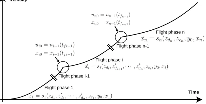
5.2.2 Decomposition of the state vector dynamics . . . 87
5.2.3 Determination of the coupling variables . . . 88
5.2.4 Proposition of the optimization strategy . . . 89
5.3 Stage-wise decomposition formulations . . . 91
5.3.1 First formulation . . . 91
5.3.2 Second formulation . . . 93
5.3.3 Third formulation . . . 95
5.3.4 Fourth formulation . . . 96
5.4 Conclusion . . . 98
6 Application case : optimization of a three-stage-to-orbit launch vehicle 99 6.1 Introduction . . . 99
6.2 Description of the disciplines . . . 100
6.2.1 Propulsion . . . 100
6.2.2 Aerodynamics . . . 102
6.2.3 Trajectory . . . 102
6.2.4 Mass budget and geometry design . . . 106
6.3 Optimization variables and disciplinary interactions . . . 109
6.3.1 Optimization variables . . . 109
6.3.2 Interactions between the different disciplines . . . 109
6.4 MDO problem formulation . . . 110
6.4.1 Initial formulation . . . 110
6.4.2 MDF formulation . . . 110
6.5 Stage-wise decomposition formulations . . . 111
6.5.1 First formulation . . . 111
6.5.2 Second formulation . . . 113
6.5.3 Third formulation . . . 114
6.5.4 Fourth formulation . . . 115
6.6 Conclusion . . . 116
7 Comparison of the different formulations 117 7.1 Introduction . . . 117
7.2 Analysis of the problem dimensionality and the number of constraints . . . . 118
7.3 Qualitative comparison of proposed formulations . . . 120
7.4 Numerical comparison of the formulations . . . 122
7.4.1 Context . . . 122
7.4.2 Adaptation of stage-wise formulations to genetic algorithm . . . 124
7.5 Conclusion . . . 132
III
Optimization strategies dedicated to the stage-wise
decom-position
135
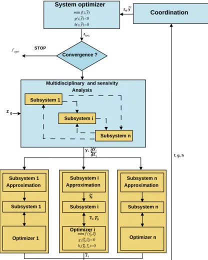
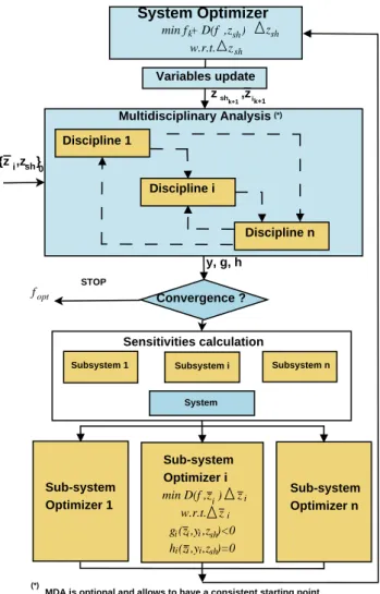
8 Optimization strategies 137 8.1 Introduction : needs and context . . . 1378.2 Description of the proposed optimization strategy . . . 138
8.3 Phase I : Exploratory phase - initialization process . . . 140
8.3.1 Exploratory phase : search of a feasible initialization at the system level140 8.3.2 Initialization process at the subsystem level . . . 141
8.4 Phase II : first optimization phase . . . 142
8.4.1 Phase II (a) : first optimization phase using the Nelder & Mead algorithm142 8.4.2 Phase II (b) : first optimization phase using the Efficient Global Op-timization algorithm . . . 143
8.5 Phase III : second optimization phase . . . 144
8.5.1 Description of the optimization phase . . . 144
8.5.2 Expression of the system level sensitivities . . . 145
8.6 Convergence considerations . . . 149
8.7 Conclusion . . . 151
9 Analysis of the optimization strategy 153 9.1 Introduction . . . 153
9.2 Determination of the reference design . . . 154
9.3 Analysis of phase I : initialization strategy . . . 157
9.4 Analysis of phase II : first optimization phase . . . 158
9.4.1 Comparison of Nelder & Mead and Genetic Algorithm . . . 158
9.4.2 Analysis of the Efficient Global Optimization algorithm . . . 159
9.5 Analysis of phase III : second optimization phase . . . 161
9.5.1 Accuracy of the gradient estimation . . . 161
9.5.2 Performance of the proposed gradient-based approach . . . 161
9.6 Analysis of the whole optimization process . . . 163
9.7 Optimization process efficiency . . . 166
9.8 Conclusion . . . 167
Conclusion
169
A Dry mass sizing module 173 A.1 Tanks . . . 173A.2 Turbopumps . . . 175
A.3 Pressurant system . . . 176
A.4 Combustion chamber . . . 177
B MDF robustness study and considerations about the Fixed Point Iteration181
B.1 Robustness of the MDF method . . . 181
B.2 Considerations about the use of the Fixed Point Iteration . . . 182
C Global Sensitivity Equation and Post-Optimality Analysis 183 C.1 Global Sensitivity Equation . . . 183
C.2 Post-Optimality Analysis . . . 184
D Demonstration of optimality conditions 187 D.1 KKT conditions for the AAO formulation . . . 187
D.2 KKT conditions for the first formulation . . . 189
D.3 Equivalence between the first and the third formulations . . . 193
E Résumé étendu de la thèse 197 Introduction . . . 197
E.1 Panorama des méthodes MDO utilisées dans la conception de lanceurs . . . 199
E.1.1 Formulation d’un problème MDO et concepts généraux . . . 200
E.1.2 Description du problème de conception de lanceurs . . . 201
E.1.3 Méthodes MDO classiques . . . 202
E.1.4 Synthèse comparative de l’application des méthodes MDO dans la con-ception de lanceurs . . . 204
E.2 Formulations MDO utilisant une décomposition en étages . . . 206
E.2.1 Introduction . . . 206
E.2.2 Présentation des formulations SWORD . . . 207
E.2.3 Présentation du cas d’application . . . 208
E.2.4 Comparaison des différentes formulations à MDF . . . 212
E.2.5 Conclusion . . . 214
E.3 Stratégie d’optimisation dédiée à la décomposition en étages . . . 214
E.3.1 Identification des besoins . . . 214
E.3.2 Description de la stratégie d’optimisation . . . 215
E.3.3 Analyse des performances de la stratégie d’optimisation . . . 218
Conclusion . . . 219
F Publications and communications 223
References
225
1 Classical Launch Vehicle Design decomposition . . . 19
1.1 Used nomenclature . . . 25
1.2 Disciplinary analyzer and disciplinary evaluator . . . 28
2.1 MDF method . . . 35 2.2 IDF method . . . 37 2.3 AAO method . . . 39 2.4 CO method . . . 42 2.5 MCO method . . . 44 2.6 CSSO method . . . 46 2.7 BLISS method . . . 48 2.8 BLISS2000 method . . . 49 2.9 ATC method . . . 50
3.1 Nelder and Mead algorithm . . . 57
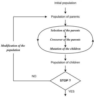
3.2 Basic scheme of an evolutionary algorithm . . . 58
3.3 Different ways to perform the crossover . . . 59
3.4 Example of mutation . . . 59
3.5 Example of kriging model . . . 61
3.6 Single shooting vs multiple shooting methods for a four-section trajectory . . 68
3.7 Interpolation using Lagrange polynomials . . . 69
5.1 Decomposition of the state vector dynamics . . . 88
5.2 SWORD formulations . . . 98
6.1 Propulsive parameters models . . . 101
6.2 Drag coefficient as a function of the Mach number . . . 102
6.3 Earth-centered, Earth-fixed reference frame . . . 104
6.4 Example of control law . . . 106
6.5 Dry mass sizing module . . . 107
6.6 Evolution of the load factor coupling coefficient with respect to the maximal axial load factor . . . 108
6.7 Results obtained with dry mass model . . . 108
7.1 Search domain and number of constraints at the system level w.r.t. the
num-ber of stages . . . 119
7.2 Statistical results of the comparison . . . 126
7.3 Results obtained for the 8th random initialization . . . . 127
7.4 Average improvement of the objective function during the optimization . . . 130
7.5 Representation of the qualitative comparison with a radar chart . . . 131
7.6 Average best found design and elapsed time to find a first feasible design . . 132
8.1 Optimization strategy . . . 139
8.2 Exploration strategy . . . 141
8.3 Initialization at the subsystem level . . . 142
8.4 Handling of design and coupling variables . . . 145
9.1 Representation of the optimal trajectory . . . 154
9.2 Optimal trajectory and geometry . . . 156
9.3 Evolution of the objective function around the reference optimum . . . 156
9.4 Search domain of the position and velocity coupling variables . . . 157
9.5 Comparison of Genetic and Nelder & Mead algorithms . . . 158
9.6 Results obtained with EGO . . . 160
9.7 Real map (2500 points) and kriged maps (50 points) around the optimum . . 161
9.8 Synthesis of the results obtained for the different phases . . . 165
9.9 Example of phase III algorithm’s behavior . . . 165
9.10 Evolution of the objective function during the optimization process . . . 166
9.11 Evolution of the objective function during the optimization using EGO and gradient-based algorithm . . . 166
A.1 Tank sizing module . . . 173
A.2 Turbopumps sizing module . . . 175
A.3 Pressurant system sizing module . . . 176
A.4 Combustion chamber sizing module . . . 177
A.5 Propulsive parameters . . . 178
A.6 Nozzle sizing module . . . 179
C.1 Coupled system . . . 183
E.1 Principe général de SWORD . . . 207
E.2 Formulations SWORD : hiérarchique (gauche) et non hiérarchique (droite) . 208 E.3 Diagramme N2 . . . 209
E.4 Dimension de l’espace de recherche et nombre de contraintes . . . 212
E.5 Comparaison des méthodes dans le cas d’une recherche globale . . . 213
E.6 Synthèse des résultats obtenus . . . 213
E.7 Stratégie d’optimisation . . . 215
E.8 Stratégie d’exploration . . . 216
E.9 Processus d’optimisation en phase 3 . . . 217
E.10 Comportement du processus d’optimisation . . . 218
1.1 Different feasibility concepts and corresponding involved variables . . . 29
2.1 Qualitative synthesis of the single level methods . . . 40
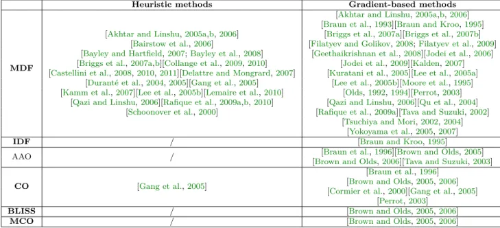
4.1 Different MDO methods applied to launch vehicle design . . . 72
4.2 Different study cases of the MDO methods . . . 73
5.1 Characteristics of the proposed formulations . . . 98
7.1 Synthesis of the optimization problems complexity at the system level . . . . 119
7.2 Search space dimension and number of constraints at the system and subsys-tem levels . . . 120
7.3 Qualitative comparison of the different formulations . . . 120
7.4 Bounds of the optimization variables . . . 123
7.5 Used GA parameters for the comparison . . . 125
7.6 Average number of generations required to find a feasible design . . . 129
7.7 Qualitative synthesis of the comparison . . . 131
9.1 Variables for the reference optimum design . . . 155
9.2 Comparison between global random and proposed initialization process . . . 157
9.3 EGO parameters . . . 159
9.4 Accuracy of the gradient estimation . . . 162
9.5 Results obtained for the validation of the second optimization phase . . . 162
9.6 Results obtained for the phase I . . . 163
9.7 Results obtained for the phase II . . . 164
9.8 Results obtained for phase III . . . 164
9.9 Summary of the results . . . 165
9.10 Dispersion of the found designs . . . 166
B.1 Results of the MDF robustness study . . . 181
B.2 Results of the Fixed Point Iteration study . . . 182
E.1 Différents concepts de faisabilité et variables associées . . . 201
MDO variables
z Design variables
y Coupling variables
x State variables
MDO functions and constraints c Coupling functions
f Objective function
g Inequality constraints
h Equality constraints
R Residuals
X State variable computation functions
J Subsystem-level intermediary objective functions
s State dynamics functions
Launch vehicle design variables
D Stage diameter
Dne Nozzle exit diameter
Isp Specific impulse
M p Propellant mass
M d Dry mass
nf Axial load factor
P c Chamber pressure
P e Nozzle exit pressure
q Mass flow rate
Rm Mixture ratio T
W Thrust to weight ratio
Trajectory variables
r Radius
v Velocity
u Control
α Angle of attack
γ Flight path angle
Notations
zsh Shared design variables ¯
zk Design variables specific to the kth subsystem
z∗ Local copies of z ˜
z Approximation of z
z◦ Feasible z
zd Design variables present in the subsystem database b
z Estimation of z
zd Design variables
zc Control variables
zd0i Design variables of the ith stage intervening in other stage dynamics
Xc State variable computation functions ensuring the consistency of the couplings ¯
x Mean value of x
σx Standard deviation of x
AAO All At Once
AT C Analytical Target Cascading
BLISS Bi-Level Integrated System Synthesis
CO Collaborative Optimization
CSSO Concurrent SubSpace Optimization
DIV E Discipline Interaction Variable Elimination
EGO Efficient Global Optimization
ELV Expendable Launch Vehicle
F D Finite Differences
F P I Fixed Point Iteration
GA Genetic Algorithm
GAGGS Genetic Algorithm Guided Gradient Search
GLOW Gross Lift-Off Weight
GSE Global Sensitivity Equation
GT O Geostationary Transfer Orbit
IDF Individual Discipline Feasible
KKT Karush-Kuhn-Tucker
LDC Local Distributed Criteria
LH2 Liquid Hydrogen
LOX Liquid Oxygen
LV D Launch Vehicle Design
M CO Modified Collaborative Optimization
M DA MultiDisciplinary Analysis
M DF MultiDiscipline Feasible
M DO Multidisciplinary Design Optimization
M DOIS Multidisciplinary Design Optimization based on Independent Subspaces
M OP CSSO Multi-Objective Pareto Concurrent SubSpace Optimization
M ST O Multi Stage To Orbit
N AN D Nested ANalysis and Design
N LP Non Linear Programming
OBD Optimization Based Decomposition
P OA Post-Optimality Analysis
P OST Program to Optimize Simulated Trajectories
P SO Particle Swarm Optimization
RP Rocket Propellant
RSM Response Surface Method
SA Simulated Annealing
SAN D Simultaneous ANalysis and Design
SQP Sequential Quadratic Programming
SN N Single NAND NAND
SSA System Sensitivity Analysis
SSN Single SAND NAND
SSS Single SAND SAND
SST O Single Stage To Orbit
Since the beginning of the XXth century and the works of Konstantin Tsiolkovsky concerning the multi stage rocket design, published in 1903 in “The Exploration of Cosmic Space by Means of Reaction Devices” , the design of launch vehicles has been constantly growing and has become a strategic domain for it enables the access to space. Launch Vehicle Design (LVD) is a very complex optimization process in which the slightest mistake may induce eco-nomical, material and human disastrous consequences (e.g. explosion of the brazilian VLS launch vehicle in 2002). This sector, due to the development of many new launch vehicles over the last few years, has been becoming more and more competitive. For this reason, it is primordial to be able to design more and more efficient launch vehicles i.e. able to put into orbit ever increasing payloads at the lesser cost, ensuring an acceptable level of reliability at the same time. This requires in early design studies an efficient optimization process so as to explore a very large search space in order to quickly obtain an appropriate launch vehicle configuration which meets the given mission requirements.
LVD involves numerous disciplines such as aerodynamics, structure, trajectory, mass budget, etc. These disciplines require specific tools and may result in conflicting decisions. For instance, the choice of a large stage diameter has antagonistic effects on launcher per-formance through aerodynamics and structural sizing. This induces a very complex design process which includes the search of multidisciplinary compromises. Therefore, in addition to the mastery of disciplinary technologies, LVD requires system-oriented design methodolo-gies in order to organize the design process.
The classical engineering design method used in LVD consists of a loop between the different disciplinary tasks. At each iteration of this loop, each discipline is reoptimized according to the data given by the previous discipline. It gives to the next discipline new data, in function of the results obtained during its own optimization. Thus, this design process needs several iterations to converge, may present some problems in order to find (if necessary) the compromises between the disciplines and may not lead to the global optimal design. Consequently, LVD requires the use of adapted tools in order to exploit the couplings between the different disciplines, to make the compromise search easier, and to improve the robustness and the efficiency of the whole design process.
Multidisciplinary Design Optimization (MDO), is a research field of engineering sciences which aims at elaborating design methodologies devoted to solving complex multidisciplinary design problems. To this end, MDO regroups several topics such as the elaboration of new design problem formulations, the creation and the use of meta models in order to reduce the calculation time, the handling of uncertainties in order to improve the robustness or the
elaboration of new optimization algorithms when the classical algorithms are inefficient. Many MDO methods can be found in literature [Balling and Sobieszczanski-Sobieski,
1994;Alexandrov and Hussaini,1995;Sobieszczanski-Sobieski and Haftka, 1997;Agte et al.,
2009; Tosserams et al., 2009]. These methods can be decomposed into two categories, with regard to the presence of one or several optimization levels.
The most used MDO method in LVD is the MultiDiscipline Feasible (MDF) method [Duranté et al., 2004; Tsuchiya and Mori, 2004; Bayley and Hartfield, 2007]. This single level method splits up the design problem according to the different disciplines and asso-ciates a global optimizer (system level) and disciplinary analysis tools (subsystem level). In order to ensure the consistency of the couplings, this method involves at the subsystem level a multidisciplinary analysis (MDA). The MDF method makes the search of the global optimum easier with respect to the classical engineering method because it uses a single optimizer which handles all the design variables. Moreover, this method allows the search of disciplinary compromises, thanks to the use of the MDA. Nevertheless, the handling of all the design variables by the single optimizer may induce a very large search space. This may pose several problems such as the requirement of an appropriate initialization and a good knowledge of the design variable search domain in order to converge. Therefore, this method is only adapted to small design problems for which the search domain can be well known in advance.
In order to address more important design problems, some MDO methods involving several levels of optimization have been proposed. These methods (e.g. Collaborative opti-mization and its derivatives [Braun and Kroo,1995;Alexandrov and Lewis,2000;DeMiguel and Murray, 2000], Bi-Level Integrated Systems Synthesis [Sobieszczanski-Sobieski et al.,
1998,2000], etc.) decompose the design problem according to the different disciplines. They use disciplinary optimizers at the subsystem level and a global optimizer at the system level in order to coordinate the different disciplinary optimizations while optimizing the global objective function.
LVD is a specific MDO problem. Indeed, it involves a dynamical system to optimize and combines the optimizations of the design variables and the trajectory. The trajectory optimization induces a trajectory simulation with stage separations. This latter involves a highly non linear ordinary differential equation system which is complex to integrate. Moreover, the trajectory is coupled with all the other disciplines and is subjected to strict equality constraints, due to the mission requirements. These constraints are very difficult to satisfy and considerably limit the feasible search domain i.e. the domain for which all the constraints are satisfied.
All the MDO methods applied to LVD in literature use a decomposition of the design problem into the different disciplines (Fig. 1). In such a decomposition, the trajectory is most often considered as a black box for the optimizer and is optimized in the same way as the other disciplines. Therefore, this decomposition may not be the most adapted to the specific LVD problem. Another decomposition of the design problem which exploits the couplings between the trajectory and the design variable optimization seems to be a valuable way of improvement of the whole optimization process.
specifications of mission coupling constraints Propulsion Structure Cost estimation Aerodynamics
Weights and Sizing
Trajectory
Recurrent cost Development cost Insurance cost Other costs
Figure 1: Classical Launch Vehicle Design decomposition
This thesis is focused on the elaboration of new MDO methods dedicated to LVD. These methods, called Stage-Wise decomposition for Optimal Rocket Design (SWORD), allow to place the trajectory optimization at the center of the design process. The SWORD methods transform the initial complex design optimization problem into the coordination of smaller single stage MDO problems, which are easier to solve. To this end, new MDO formulations of the LVD problem and an associated optimization strategy are proposed. The SWORD methods are analyzed and compared to the most used MDO method in literature (MDF).
This manuscript is organized into three parts. The first part is devoted to drawing up a panorama of the MDO methods used in LVD. Chapter 1presents the fundamental concepts used to describe a general MDO process. In Chapter 2, we detail the main MDO methods applied in LVD. Chapter 3 concerns the description of the main optimization algorithms used in MDO and the different techniques employed to perform the trajectory optimization. Finally, Chapter 4 details the analysis of the application of the MDO methods in LVD, and expresses some possible ways of improvement with regard to this specific MDO problem.
The second part of this document is related to the description and the analysis of the proposed MDO formulations. To this end, we express in Chapter 5four MDO formulations in order to solve the LVD problem. Chapter6is devoted to the description of the application case selected in this study : the optimization of three-stage-to-orbit launch vehicle for the minimization of the Gross-Lift-Off-Weight. Finally, Chapter 7 compares the SWORD for-mulations with the most used MDO method, theoretically and numerically in case of global search study.
The last part of this document is devoted to the description and the analysis of the proposed optimization strategy dedicated to the SWORD formulations. To this end, this part is organized into two chapters. Chapter8 concerns the elaboration of the optimization strategy. In this chapter, we detail the different parts of the optimization strategy and we describe the proposed optimization algorithms. Finally, Chapter 9 describes the numerical analysis of the optimization strategy. In this chapter, we analyze each of the optimization strategy phases and we study the performance of the whole optimization process (i.e. MDO formulation and optimization algorithms), in terms of calculation time, quality of the op-timum and robustness to the initialization. Finally, we conclude on the efficiency of the SWORD methods, their use in Launch Vehicle Design preliminary studies and we detail several ways of improvement.
The appendices present some model considerations concerning the application case, and detail some optimization techniques and mathematical demonstrations used in Chapter 8. The last appendix is constituted of an extended abstract of this thesis written in French.
Panorama of Multidisciplinary Design
Optimization methods used in Launch
Generalities about Multidisciplinary
Design Optimization
Contents
1.1 Introduction . . . . 23
1.2 Mathematical formulation of the general MDO problem . . . . 24
1.2.1 Problem formulation . . . 25 1.2.2 Types of variables . . . 25 1.2.3 Types of constraints . . . 26 1.2.4 Types of functions . . . 26 1.2.5 Disciplinary equations . . . 26 1.2.6 Coupling . . . 27 1.2.7 Multidisciplinary analysis . . . 28
1.3 Feasibility concepts in MDO . . . . 28
1.3.1 Individual disciplinary feasibility . . . 28
1.3.2 Multidisciplinary feasibility . . . 29
1.4 Description of the Launch Vehicle Design problem . . . . 29
1.4.1 Disciplines and variables . . . 29
1.4.2 Constraints . . . 30
1.4.3 Objective functions . . . 30
1.4.4 Specificities of the Launch Vehicle Design problem . . . 30
1.5 Conclusion . . . . 31
1.1
Introduction
Multidisciplinary Design Optimization (MDO), also named Multidisciplinary Optimization
is a relatively recent field of engineering sciences whose objective is to address more effi-ciently design problems incorporating different disciplines. The MDO has been used in a great number of domains such as structure, automotive, electronics or aerospace engineering, and allows to solve complex problems which are difficult to handle with the classical design methods. This research field could grow up thanks to the increase of computation power in the second half of the XXth century. Indeed, this increase has made the numerical
opti-OPTIMIZATION mization of complex problems possible and has paved the way for the complete system design. By handling the different disciplines simultaneously, the MDO techniques facilitate the search of the global optimal design, which might not be obtained when the disciplines are handled sequentially. Indeed, in most of the design problems, the different disciplines may lead to antagonistic decisions (e.g. structure and aerodynamics in launch vehicle design, as we shall see later). In such cases, the MDO techniques aim to find compromises between the different disciplines in order to reach the global optimal design.
Handling at the same time a series of disciplines increases significantly the complexity of the problem to solve. One of the branches of the MDO field is dedicated to the elaboration of new formulations of the optimization problem which aim at reducing the complexity of the problem and at allowing the more efficient use of the traditional optimization methods. The works presented in this document lie within this scope.
Instead of disciplinary codes in a computer or computer networks, the MDO may also address design problems involving engineer teams all over the world. Indeed, due to the glob-alization of the industries, the system design can be split up into different research centers located in different countries. In this case, the data exchanges between the teams become a crucial point of the design process and MDO provides new tools for the designers in order to make the design process more efficient.
This part is devoted to the description of the application of the MDO methods to the Launch Vehicle Design. The first chapter of this part concerns the presentation of the fun-damental concepts necessary to describe a MDO process. In the second chapter, we present the main MDO methods used in literature. The third chapter concerns the description of the classical optimization algorithms used in a MDO process and the main optimal control methodologies. Finally, in the fourth chapter, we analyze the application of the MDO meth-ods in Launch Vehicle Design in order to compare the different presented methmeth-ods and to propose several ways of improvement.
1.2
Mathematical formulation of the general MDO
problem
In this section, we define the fundamental notions necessary to describe a classical MDO process. The Launch Vehicle Design problem can be decomposed into different ways. These decompositions imply different optimization architectures. Indeed, the different disciplines can be considered separately or can be optimized simultaneously inside a same system. Hereinafter, we will use, with the same signification, both terms discipline and subsystem, in order to describe the different processes at the subsystem level (Fig. 1.1). A subsystem may regroup several disciplines and can be a part of a system to optimize (e.g. a stage of a launch vehicle). In this section, we firstly describe the general mathematical formulation of a MDO problem and then we expose the different involved variables, functions and constraints. Finally, we detail the different ways to handle the disciplinary equations and couplings.
1.2.1
Problem formulation
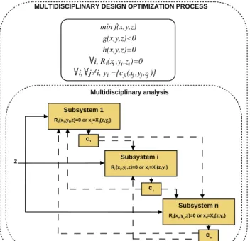
The general formulation of a MDO problem can be written as follows :
Formulation I.1 (General MDO formulation)
Minimize f (x, y, z) With respect to z ∈ Z Subject to g(x, y, z) ≤ 0 (1.1) h(x, y, z) = 0 (1.2) ∀i ∈ {1, · · · , n}, ∀j 6= i, yi = {cji(xj, yj, zj)}j (1.3) ∀i ∈ {1, · · · , n}, Ri(xi, yi, zi) = 0 (1.4) A general MDO process is illustrated in Figure 1.1. All the different variables and functions intervening in the MDO process will be described in the following sections.
Subsystem 1 z min f(x,y,z) g(x,y,z)<0 h(x,y,z)=0 i, R (x ,y ,z )=0 i, j=i, y ={c (x ,y ,z )}
MULTIDISCIPLINARY DESIGN OPTIMIZATION PROCESS
R (x ,y ,z)=0 or x =X (z,y )1 11 Multidisciplinary analysis i i i i ji j j j i c1 cn ci 1 1 1 Subsystem i R (x ,y ,z)=0 or x =X (z,y )i i i i i i Subsystem n R (x ,y ,z)=0 or x =X (z,y )n nn n n n
Figure 1.1: Used nomenclature
1.2.2
Types of variables
A general MDO process involves several types of variables. These variables play specific roles and are used at the different steps of the MDO process. We can differentiate three categories of variables in a general MDO problem:
• z : design variables. These variables evolve all along the optimization process in order to find the optimal design. They can be used in one or several subsystems:
OPTIMIZATION
z = {zsh, ¯zk}. The subscript sh stands for the variables which are shared between different subsystems (global variables) and ¯zk denotes the variables which are specific to one subsystem (local variables). Moreover, we use the notation zk to describe the variables which refer to the kth subsystem.
• y : coupling variables. These variables are used to link the different subsystems and to evaluate the consistency of the design with regard to the coupling.
• x : state (or disciplinary) variables. These variables (which are not the design variables) can vary during the disciplinary analysis in order to find an equilibrium in the state equations (disciplinary equations). Unlike z, the state variables are not independent degrees of freedom but depend on the design variables z, the coupling variables y and the state equations. The cases in which x are given by explicit functions of z and y are uncommon in engineering applications. Indeed, these variables are most often defined by implicit functions, that generally require specific optimization methods for solving complex industrial problems.
1.2.3
Types of constraints
The constraints can be divided in two categories : • g : inequality constraints,
• h : equality constraints.
1.2.4
Types of functions
The different functions used in a MDO problem are :
• f (x, y, z) : objective function. This function quantifies the quality of the design and has to be optimized by the MDO process.
• c(x, y, z) : coupling functions. These functions are used to compute the coupling variables which come out of a subsystem. We will note cij(xi, yi, zi) the coupling variables from the subsystem i to the subsystem j.
• Ri(xi, yi, zi) : residual functions. The residuals quantify the satisfaction of the state equations (1.4).
• Xi(yi, zi) : state variable computation functions. These functions yield the roots xi of the equations (1.4).
1.2.5
Disciplinary equations
• Non-residual form (explicit):
xi = Xi(yi, zi) (1.5)
In this case, the state variables can be explicitly determined from the design and cou-pling variables.
• Residual form (implicit) :
Ri(xi, yi, zi) = 0 (1.4) In this form, there is no explicit relation to determine the state variables from the design and coupling variables.
We can distinguish two methods for handling the disciplinary equations (Fig. 1.2) :
Disciplinary analysis
Definition 1.2.1. Given the design and coupling variables (respectively zi and yi), the
dis-ciplinary analysis consists in finding the values of the state variables xi such that the state
(disciplinary) equations Ri(xi, yi, zi) = 0 are satisfied.
Generally, when the disciplinary equations are expressed in the residual form, a specific solver (e.g. a Newton algorithm) is used in order to find the roots of the equations (1.4). When the non residual-form is used, the iterative loop is not required in the subsystem because the state variables are directly expressed from the design and coupling variables by explicit relationships. In this case, the calculation scheme consists in sequentially evaluating the different relationships in order to compute the disciplinary outputs (Eq. 1.5).
Disciplinary evaluation
Definition 1.2.2. Given the design, coupling and state variables (respectively zi, yi and xi),
the disciplinary evaluation consists in calculating the value of the residuals Ri(xi, yi, zi). In this scheme, the equations (1.4) are not solved. Furthermore, the state variables x are not handled in the subsystem but are considered as inputs in the same way as z and y. The disciplinary evaluation just computes the value of Ri but does not solve the equations
Ri = 0. Consequently, in case of residual form, this process takes much less computation time than the disciplinary analysis.
As we shall see later, this dichotomy in the way to handle the disciplinary equations is the principal difference between the All At Once and the Individual Discipline Feasible formulations.
1.2.6
Coupling
From the variables yiand zi coming in the subsystem i and the state variables xi, the coupling variables which come out of the subsystem can be calculated with the coupling functions
OPTIMIZATION Subsystem analysis x | R (x ,y ,z )=0 or x = X (z ,y ) z , y x Subsystem evaluation z , y , x R (x ,y ,z )=? x ,y ,z c (x ,y ,z ) c (x ,y ,z ) DISCIPLINARY EVALUATOR DISCIPLINARY ANALYZER i i i i i i i i i i i i i i i i i i i i i i i i i i i i i i c (x ,y ,z )i i i i c (x ,y ,z )i i i i
Figure 1.2: Disciplinary analyzer and disciplinary evaluator
transmitted from the ith subsystem to the jth subsystem. The coupling is consistent when the set of coupling variables yi is equal to the set returned by the different coupling functions (Eq. 1.3).
1.2.7
Multidisciplinary analysis
Definition 1.2.3. The MultiDisciplinary Analysis (MDA) is a process which aims to sat-isfy the individual disciplinary feasibilities and the consistency of the couplings between the different subsystems. The MDA consists in finding, for all the subsystems, the variables xi
and yi such that the state equations are satisfied and the couplings are consistent.
In other words, the MDA consists in satisfying the system formed by the equations (1.3) and (1.4), as follows :
(
∀i ∈ {1, · · · , n}, ∀j 6= i, yi = {cji(xj, yj, zj)}j ∀i, ∈ {1, · · · , n}, Ri(xi, yi, zi) = 0
A classical way to perform the MDA is to use the Fixed Point Iteration (FPI). The FPI generally consists of a loop between the different disciplinary analyses (each of them finding the state variables x in order to make the disciplinary residuals zero). This technique requires some properties of the coupling function and may not converge if the considered function is not contractive [Banach,1922]. Different numerical schemes of the MDA (Gauss-Seidel and Gauss-Jacobi, etc.) are developed in details in [Keane and Nair, 2005].
1.3
Feasibility concepts in MDO
We can distinguish two feasibility concepts in MDO. These concepts are related to the feasibility of either only one subsystem or all the subsystems.
1.3.1
Individual disciplinary feasibility
Definition 1.3.1. A process is qualified as “individual disciplinary feasible” [Cramer et al., 1994] if at each iteration, the state equations of the different disciplines are satisfied.
In other words, the individual disciplinary feasibility means that we are always able to find the values of the state variables x which satisfy the equations (1.4) (but the consistency of the couplings is not guaranteed). Trivially, a process in which all the disciplinary equations are in the non-residual form (Eq. 1.5) is intrinsically “individual disciplinary feasible” .
1.3.2
Multidisciplinary feasibility
Definition 1.3.2. A process is qualified as “multidisciplinary feasible” [Cramer et al., 1994] if at each iteration, the state and coupling variables (respectively xi and yi) can be found
such that the “individual disciplinary feasibility” is realized and the couplings are consistent.
A problem in which a MDA is performed is a “multidisciplinary feasible” problem. In this kind of problems, we can express the values of the state variables exclusively in function of the design variables : x = Xc(z) (the subscript c stands for the consistency of the coupling). Table 1.1 summarizes the level of centralization and the different degrees of feasibility of a MDO process.
Concept Process used at Variables handled Variables handled subsystem level by the subsystems outside the subsystems No feasibility ensured Disciplinary evaluation x,y,z
Individual disciplinary feasibility Disciplinary analysis x y,z
Multidisciplinary feasibility MDA x,y z
Table 1.1: Different feasibility concepts and corresponding involved variables
As we will see in Chapter 2, these two feasibility concepts are the principal difference between the Multi Discipline Feasible and the Individual Discipline Feasible formulations.
1.4
Description of the Launch Vehicle Design problem
In this section, we briefly present the Launch Vehicle Design (LVD) problem. To this end, we describe the different disciplines, variables and constraints involved in such a problem, and we point out the specificities of this design problem with respect to other MDO problems. A launch vehicle is a specific vehicle which aims to put a payload in a certain orbit. A launch vehicle is a dynamical system which moves using rocket propulsion and involves a multi stage architecture. The different stages of the launch vehicle are jettisoned during the flight. These stages can land on Earth (e.g. the boosters), enter in the atmosphere (e.g. the intermediary stages) or remain in space (e.g. the last stage).1.4.1
Disciplines and variables
The Launch Vehicle Design problem is generally decomposed into the different physical disciplines. The classical disciplines involved in such design problems are :
• aerodynamics, • propulsion,
OPTIMIZATION • structure,
• costs,
• weights & sizing,
• trajectory (performances calculation).
Each of these disciplines involves its own constraints and variables. The design variables
z, such as the masses, the diameters, the propulsion variables (chamber pressures, mixture
ratios ...), the fairing shape, etc. are generally considered at the system level. The trajectory variables (variables of the control law if the trajectory optimization is computed by a direct method or adjoint vector if the optimization uses an indirect method) are usually considered as state variables x (the optimal control techniques will be described in Chapter 3). The optimality conditions associated with these variables can be satisfied at the subsystem level (R = 0) or at the system level (R = 0 added to the system level equality constraints). In this particular case, the control law variables are at the same level as the design variables z. Typical coupling variables y may be the dry mass, the stage diameters, the thrust to weight ratio, etc.
1.4.2
Constraints
The involved equality constraints h in the LVD problem may be composed of the require-ments of the mission (desired orbit, payload mass, Gross Lift Off Weight ...) and the in-equality constraints g may include for instance the maximum chamber pressure, the maximal angle of attack, the maximum load factor or the minimum nozzle exit pressure. The classical involved coupling constraints may concern the trajectory and the weights & sizing or the trajectory and the aerodynamics, etc.
1.4.3
Objective functions
The classical objective functions f are :• the maximization of the payload mass,
• the minimization of a mass (most often the Gross Lift-Off Weight or the dry mass), • the minimization of the global or recurring cost.
These objective functions are most often computed by the weight & sizing or the performance calculation (trajectory) subsystems.
1.4.4
Specificities of the Launch Vehicle Design problem
The main difference between the Launch Vehicle Design problem and the other MDO prob-lems concerns the presence of a dynamical system to optimize (trajectory optimization with stage separations). Indeed, the LVD problem combines the coupled optimizations of the design and trajectory variables. The trajectory optimization induces a trajectory simulation with stage separations which is complex to integrate (numerical resolution of a highly non linear ordinary differential equation system). Moreover, the trajectory is subjected to strict equality constraints, due to the mission specifications, which are very difficult to satisfy
and considerably limit the feasible search domain (domain for which all the constraints are satisfied). We will study more in details the specificities of the LVD problem when we will describe the application of the MDO methods in LVD in the fourth chapter of this part.
1.5
Conclusion
In this chapter, we have introduced the fundamental notions necessary to describe a MDO process. To this end, the general formulation of a MDO problem and the different vari-ables, functions and constraints involved in such problems have been detailed. From the description of the different ways to handle the disciplinary equations, the different feasibility concepts have been described. Finally, the requirements of the launch vehicle design and the main differences between such design problem and other MDO problems have been briefly described.
The different notations and the concepts introduced in this chapter will be useful in the next chapter which will be devoted to the general description of the main MDO formulations. We will also use these notations in the second part of this document in order to describe our proposed MDO methods.
Classical MDO methods
Contents
2.1 Introduction . . . . 33
2.2 Single level methods . . . . 34
2.2.1 Multi Discipline Feasible . . . 34
2.2.2 Individual Discipline Feasible . . . 36
2.2.3 All At Once . . . 38
2.3 Qualitative comparison of the single level methods . . . . 39
2.4 Multi level methods . . . . 40
2.4.1 Collaborative Optimization . . . 40
2.4.2 Modified Collaboration Optimization . . . 42
2.4.3 Concurrent SubSpace Optimization . . . 44
2.4.4 Bi-Level Integrated Systems Synthesis . . . 46
2.4.5 Analytical Target Cascading . . . 49
2.4.6 Other multi level methods . . . 51
2.5 Conclusion . . . . 52
2.1
Introduction
Since the last two decades of the XXthcentury, a lot of MDO methods have been proposed in the literature. Indeed, many authors such as Sobieski, Braun, Cramer, etc. have proposed new MDO formulations in order to more efficiently cope with the engineering problems they have to solve. This chapter is devoted to the description of the main MDO methods present in the literature. We can find many MDO methods which have been applied in a great number of examples. Because the study cases are different, it is difficult to com-pare these methods in order to determine which is the best. Some review articles [Balling and Sobieszczanski-Sobieski, 1994; Alexandrov and Hussaini, 1995; Sobieszczanski-Sobieski and Haftka, 1997; Agte et al., 2009; Tosserams et al., 2009] provide a state-of-the-art of the different MDO methods. The aim of this chapter is not to make an exhaustive list of the different MDO methods but at first to describe the main MDO methods with common standardized notations introduced in the first chapter. One of the goals of this part is to evaluate the applicability of the expressed methods in launch vehicle design and to bring
out the advantages and the drawbacks of these methods with regard to this specific problem. This chapter is devoted to the description of the MDO methods. To this end, the chap-ter is organized as follows. In the second section, we describe the single level methods i.e. the MDO methods which only require one optimizer. The third section is devoted to the qualitative comparison of these single level methods. The fourth section concerns the de-scription of the main multi level methods (involving more than one optimizer). For each of the described methods, we expose at first the principle of the method, then its mathematical formulation accompanied by an explanatory scheme, and finally we present the advantages and drawbacks of the considered MDO method.
2.2
Single level methods
2.2.1
Multi Discipline Feasible
Principle
The Multi Discipline Feasible (MDF) method is the most usual MDO method. It is also called “Nested Analysis and Design” (NAND), “Single NAND-NAND” (SNN) and “All-in-One”. This method is explained in [Balling and Sobieszczanski-Sobieski,1994;Cramer et al.,
1994; Kodiyalam, 1998; Allison, 2004; Gang et al., 2005]. The architecture of the MDF method is similar to the architecture of a classical optimization problem which involves only one subsystem. The main difference is that, in MDF, the subsystem is replaced by a complete multidisciplinary analysis which is performed at each iteration of the optimization process. Thus, all the subsystems are coupled in an analysis module which ensures the multidisci-plinary feasibility of the solution at each iteration (Fig. 2.1). In this formulation, the set of design variables is transmitted to the analysis module. This module executes, by a dedicated method (e.g. Fixed Point Iteration or Newton method), the multidisciplinary analysis of the system (1.3)-(1.4).
Formulation I.2 (MDF formulation)
Minimize f (Xc(z), y, z)
With respect to z ∈ Z
Subject to g(Xc(z), y, z) ≤ 0 (2.1)
h(Xc(z), y, z) = 0 (2.2)
Once the MDA is performed, the analysis module output vector is used by the system level optimizer to compute the objective function and the constraints. The process is re-peated at each iteration. In this method, each set of found design variables is a consistent configuration. Furthermore, the disciplines are in charge of finding their local variables x to satisfy their own equations (1.4) (disciplinary analyzers are used). In this manner, the state variables do not intervene in the optimization problem formulation because they are totally handled by the disciplinary analyzers during the MDA at the subsystem level. In the
MDF method, each found solution is multidisciplinary feasible (i.e. individual disciplinary equations (1.4) as well as coupling equations (1.3) are satisfied). We can note that the term “multidisciplinary feasible” does not imply the satisfaction of design constraints g and h, but only the MDO ones.
Some systems do not present any feedback between the different subsystems (i.e. [ Du-ranté et al., 2004], [Castellini et al., 2010]). In this case, a sequential analysis, without iteration, is possible and the MDF method is the most natural method to solve this kind of problems. Indeed, for these problems, the coupling constraints (Eq. 1.3) are automatically satisfied by the sequential calculation process.
For large scale (industrial) application cases, the different subsystem disciplinary analyses can be composed of groups of specialists (each of them potentially located in a different place all over the world). In this case, the MDA becomes a very complex task and includes :
• transmission of informations between the different groups of specialists (dotted lines in Figure 2.1), and not only between computers or optimization programs,
• management requirements between and inside the different groups (because each group potentially converses with all the others),
• definition of each group action domain and autonomy with respect to the community (in order to ensure as much as possible the consistency of the trade-off establishments).
Subsystem 1 analyzer Subsystem i analyzer Subsystem n analyzer Multidisciplinary analysis
Optimizer
z f,g,h x x x 1 i n min f(Xc(z),y,z) g(Xc(z),y,z)<0 h(Xc(z),y,z)=0 R (x ,y ,z )=0 or x =X (y ,z ) i i i i i i i i 1i y Figure 2.1: MDF methodAdvantages and drawbacks of MDF
The main advantage of the MDF method is its simplicity. Indeed, a limited number of opti-mization variables is used (only the design variables z have to be handled by the optimizer) and classical disciplinary analyzers are used. The method implementation is relatively easy since the system decomposition is not required. Moreover, if the optimization process is stopped, the found solution is consistent with respect to the couplings and the individual disciplinary feasibilities, even if it is not the optimal one.
The MDF method presents important drawbacks. Indeed, the calculation cost is very important and the method does not take advantages of the couplings between the disciplines in order to improve the optimization process, because the optimizer does not control the choices performed by the MDA, which is considered as a black box. The calculation cost is due to the MDA which has to be executed at each iteration of the optimization process. This analysis considers all the subsystems present in the MDO process (the MDF method modularity is very poor). Thus, when a design variable changes, all the other variables have to be recalculated. Furthermore, a gradient-based algorithm used as the optimizer will need a full MDA whenever the derivatives required to compute the gradient or the Hessian will have to be calculated [Kodiyalam,1998]. Moreover, if the MDA is performed by a FPI, the MDA may not converge if the considered function is not contractive. Consequently, MDF is principally applicable to the optimization problems for which the different subsystems can be quickly evaluated during the MDA or for which the MDA converges in a few iterations.
For large scale application problems (in which the subsystems are engineering teams), at each iteration, the MDA requires a lot of information transmissions and management tasks because each group has to potentially converse with all the others. The MDA is also responsible for defining the action domain of each specialty group (possible conflict resolutions with engineers who want to decide design and to have as much autonomy as possible). Moreover, each group of specialists has to wait for the previous one in order to perform its task (when FPI is used), that can be very time consuming.
2.2.2
Individual Discipline Feasible
Principle
The Individual Discipline Feasible (IDF) method [Cramer et al.,1994;Martins and Marriage,
2007], also called “Optimizer-Based-Decomposition” (OBD) [Kroo, 2004], “Single-SAND-NAND” (SSN) [Balling and Sobieszczanski-Sobieski, 1994], allows to avoid a complete mul-tidisciplinary analysis at each iteration of the design process. Like MDF, a single optimizer at the system level is used and disciplinary analysis blocks are called in the different sub-systems. The main difference between MDF and IDF is that for IDF, the optimizer is also responsible for the coordination of the different subsystems and uses additional variables (coupling variables y) to ensure it. At each iteration of the optimization process, the differ-ent subsystems are individually feasible but the consistency of the couplings between them is not guaranteed. The IDF formulation of a MDO problem may be summarized as follows :
Formulation I.3 (IDF formulation)
Minimize f (X(y, z), y, z)
With respect to (y, z) ∈ Y × Z
Subject to g(X(y, z), y, z) ≤ 0 (2.3)
h(X(y, z), y, z) = 0 (2.4)
∀i ∈ {1, · · · , n}, ∀j 6= i, yi = {cji(Xj(yj, zj, ), yj, zj)}j (2.5) This method allows to break up the main problem into several subsystems. The coupling variables (and the associate coupling equations (1.3)) are introduced in order to evaluate the consistency of the results found by the different subsystem analyzers. In IDF, the consistency of the solution (multidisciplinary feasibility Eq. 1.3) is not ensured at each iteration but only at the convergence. Consequently, the IDF process should not be stopped before the convergence is reached.
This decomposition method considerably increases the number of variables handled at the system level but allows to improve the computational speed (parallelization is possible). Therefore, unlike the MDF method, a single analysis is performed at each iteration in the different subsystems. The centralization degree of the IDF method is more important than the MDF one. There again, the subsystems determine their state variables (subsystem analyzers are used).
Optimizer Subsystem 1 analyzer x1 Subsystem n analyzer xn z ,yi z ,y1 z ,yn z,y f, y - c, g, h min f(X(y,z),y,z) g(X(y,z),y,z)<0 h(X(y,z),y,z)=0 i, j=i, y ={c (x ,y ,z )} i ji j j Subsystem i analyzer xi R (x ,y ,z )=0 or x =X (y ,z ) i i i i i i f ,g , h , c i i i ij i i j 1 i n
Figure 2.2: IDF method
Advantages and drawbacks of IDF
If the number of coupling variables is relatively small, the IDF method is applicable and provides results in a limited computational time. Since the principle of this method is to introduce additional coupling variables and constraints at the system level, the number of iterations at the system level is more important than in MDF. The optimizer has to dialog with each disciplinary block and transmits to each of them its own coupling variables.
(parallelization is possible). This particularity can considerably improve the efficiency of the method (calculation time is reduced). Furthermore, since the MDA process is removed, the internal analysis loop is broken up. In this way, if the system level optimizer requires sensitivity calculations of the ith subsystem, the other subsystems do not intervene and no computation time is wasted. Therefore, if an important centralization of the optimization process is possible, the IDF method can be employed to effectively solve a MDO problem.
For large scale applications (for which the subsystems are composed of engineers), the management tasks are less important than in MDF because each group just converses with the coordinator and not with all the others. Indeed, since the MDA is broken, the different engineering teams have not to wait for the results of other teams, that allows to parallelize the human tasks. However, the autonomy of the different teams is limited because the multi disciplinary feasibility is not ensured at the subsystem level, but at the system level.
2.2.3
All At Once
Principle
The All At Once (AAO) method, also called “Single-SAND-SAND” (SSS) [Balling and Sobieszczanski-Sobieski, 1994; Balling and Wilkinson, 1997] solves simultaneously the opti-mization problem and the equations of the different subsystems [Allison, 2004]. The equa-tions (2.8), (2.9) are not satisfied at each iteration of the optimization process but they have to be at the convergence [Cramer et al., 1994] (the design configuration is consistent only at the convergence). In this method, the subsystem equations (residuals) are considered as equality constraints R = 0.
AAO is the most elementary MDO method. The control of the process is assigned to a system level optimizer which aims to optimize a global objective and calls subsystem evalu-ations. The optimizer handles the design variables z, the coupling variables y and the state variables x. At the subsystem level, the disciplinary analyzers are replaced by disciplinary evaluators. The design and the evaluations at the subsystem and system levels are performed at the same time. Therefore, the centralization of the problem is more important than in IDF and MDF. The AAO formulation of the MDO problem can be summarized as follows :
Formulation I.4 (AAO formulation)
Minimize f (x, y, z) With respect to (x, y, z) ∈ X × Y × Z Subject to g(x, y, z) ≤ 0 (2.6) h(x, y, z) = 0 (2.7) ∀i ∈ {1, · · · , n}, Ri(xi, yi, zi) = 0 (2.8) ∀i ∈ {1, · · · , n}, ∀j 6= i, yi = {cji(xj, yj, zj)}j (2.9) The global state vector is divided into subvectors which are distributed to each subsys-tem. The residuals R are transmitted to the global optimizer simultaneously with the other
variables. Since the residuals are equal to zero only at the optimum, the multidisciplinary and the individual disciplinary feasibilities are not ensured at the intermediary points.
Optimizer
Subsystem 1 evaluator Subsystem i evaluator Subsystem n evaluator x ,y , zi i f ,R ,c ,g ,hi i ij i i x ,y, z f, R, y-c, g, h min f(x,y,z) g(x,y,z)<0 h(x,y,z)=0 i, R (x ,y ,z )=0 i, j=i, y ={c (x ,y ,z )} i ji j j i i i R (x ,y ,z )=?i i i j i i iFigure 2.3: AAO method
Advantages and drawbacks of AAO
The AAO method is the less complex method to solve MDO problems because it does not make any difference between the different involved variables which are all handled at the same level. Nevertheless, AAO presents some drawbacks which make it inapplicable to large scale launch vehicle design problems. Indeed, in the case of problems which consider several complex subsystems, the number of variables handled by the optimizer soars, that makes AAO not applicable.
In the situations for which the convergence is not achieved, the AAO method (like IDF) does not provide a feasible design. Moreover, the AAO method is difficult to implement because highly centralized. This method may present some robustness difficulties because the formulation results in a very constrained MDO problem. In relatively small problems, AAO, like IDF, is applicable and allows to parallelize calculations. Thus, the computation time may be considerably reduced.
For large scale applications, the different groups of engineers do not perform the indi-vidual disciplinary analysis of the different subsystems but are just reduced to make sim-ple calculations with respect to the instructions given by the system level. Indeed, simsim-ple computations of the residuals are involved at the subsystem level, that do not require the intervention of engineering teams at this level. For this reason, the AAO method is just ap-plicable to small problems for which all the calculations can be performed by a small group of generalist engineers.