Numerical Simulation of Radiative Heat Transfer in a High Voltage Circuit Breaker

NUMERICAL SIMULATION OF RADIATIVE HEAT TRANSFER IN A HIGH VOLTAGE CIRCUIT BREAKER

ALI MAZAHERI

DÉPARTEMENT DE GÉNIE MÉCANIQUE ÉCOLE POLYTECHNIQUE DE MONTRÉAL

MÉMOIRE PRÉSENTÉ EN VUE DE L’OBTENTION DU DIPLÔME DE MAÎTRISE ÈS SCIENCES APPLIQUÉES

(GÉNIE MÉCANIQUE) AVRIL 2018

c

ÉCOLE POLYTECHNIQUE DE MONTRÉAL

Ce mémoire intitulé :

NUMERICAL SIMULATION OF RADIATIVE HEAT TRANSFER IN A HIGH VOLTAGE CIRCUIT BREAKER

présenté par : MAZAHERI Ali

en vue de l’obtention du diplôme de : Maîtrise ès sciences appliquées a été dûment accepté par le jury d’examen constitué de :

M. REGGIO Marcelo, Ph. D., président

M. TRÉPANIER Jean-Yves, Ph. D., membre et directeur de recherche M. CAMARERO Ricardo, Ph. D., membre et codirecteur de recherche M. KUMMERT Michaël, Doctorat, membre

DEDICATION

I dedicate this thesis to my parents

ACKNOWLEDGMENTS

I would like to express my sincere gratitude to my thesis supervisors Prof. Jean-Yves Trépanier and Prof. Ricardo Camarero for giving me the opportunity of working on this project, and for supporting me patiently during it.

I would also like to thank General Electric Grid Solution for their financial support, and also Dr. Philippe Robin-Jouan for his scientific advice as the senior expert for scientific simulations at General Electric Power, Grid Solution.

My sincere thanks also go to Dr. Sina Arabi, for his help during this project.

I express my sincere thanks for the support received from my friends and colleagues who helped me during these three years.

Finally, I would express a deep sense of gratitude to my parents who have supported me emotionally , and stood besides me all of my life.

RÉSUMÉ

La simulation de l’environnement thermique et la prédiction du taux d’ablation dans un dis-joncteur dépendent fortement des résultats obtenus par la simulation du rayonnement. Par conséquent, le développement d’une méthode efficace pour la simulation est d’une importance capitale. Un code robuste appelé M C3 _{a été développé à l’École Polytechnique de Montréal} depuis une trentaine d’années afin de simuler des disjoncteurs haute tension, et plusieurs méthodes ont été implémentées dans le code pour modéliser le transfert de chaleur radiatif. Cependant, chacun d’entre eux a des lacunes, ainsi un modèle plus efficace en termes de pré-cision et de temps de calcul a été nécessaire. Dans ce projet, une méthode explicite de volume fini sans procédure itérative est utilisée pour simuler le transfert de chaleur radiatif dans les disjoncteurs haute tension. Dans le présent travail, la méthode explicite, utilisant le balayage de l’espace, est mise en œuvre et plusieurs cas test sont étudiés. Afin de valider la méthode, une enceinte cylindrique classique est testée avec trois épaisseurs optiques et les résultats obtenus sont comparés aux résultats analytiques. Les résultats analytiques confirment les résultats numériques. Un disjoncteur semi-industriel est étudié avec trois épaisseurs optiques et les résultats obtenus du présent travail sont comparés aux résultats obtenus par la modèle P1 et la méthode implicite FVM (Finite Volume Method). Les résultats obtenus des deux FVM concordant. Cependant, les résultats P1 pour les cas optiquement épais et minces ne correspondent pas aux résultats du FVM. Le temps de calcul pour ces trois méthodes sont comparés. P1 est la méthode la plus rapide, tandis que le temps CPU pour le FVM expli-cite est raisonnablement proche du temps P1. La tuyère entourant l’arc dans un modèle de disjoncteur est simulée comme troisième cas test en utilisant P1 et FVM explicite pour cinq bandes de fréquence d’émission. Les résultats obtenus avec la méthode FVM sont comparés aux résultats de P1. Ces résultats sont calculés pour chaque bande afin de déterminer leur participation à la valeur totale. Des études montrent que le transfert de chaleur radiant qui atteint la paroi de la tuyère pour les trois premières bandes est négligeable et que seules les deux dernières bandes participent au rayonnement. L’effet de la condition limite de Marshak et Dirichlet sur le flux pour le modèle P1 est étudié et la valeur de l’énergie sur paroi pour les deux est comparée aux résultats obtenus de FVM. On observe que la valeur de l’énergie sur la paroi pour les conditions aux limites de Marshak est plus proche de celle obtenue de par FVM, tandis que P1 avec Marshak ne peut pas déterminer l’emplacement du flux maxi-mal qui est très important dans le calcul du taux d’ablation. Le temps CPU pour le FVM implémenté dans le présent travail est comparé à celui obtenu de P1 et on observe que P1 est plus de 10 fois plus rapide alors que les résultats FVM sont plus réalistes.

ABSTRACT

Radiation is an effective mechanism of heat transfer in a circuit breaker. Simulation of the thermal environment and the prediction of the rate of ablation in a circuit breaker are strongly dependent on results obtained from simulation of the radiative heat transfer. Therefore, the development of an efficient method to simulate this phenomenon is of vital importance. A simulation software called M C3 _{has been developed at Ecole Polytechnique de Montréal since} about 30 years ago to simulate high voltage circuit breakers, and several methods have been implemented in this code to model the radiative heat transfer. However, each of them has shortcomings, and a more efficient model in terms of accuracy and computational cost is needed. In this project an explicit finite volume method without any iterative procedure is proposed to simulate the radiative heat transfer in such devices. The explicit finite volume method (FVM) using a marching order map is implemented and applied to several test cases. For validation purposes of the implementation, a classic cylindrical enclosure is tested in three optical thicknesses and the results obtained are compared with analytical results which confirm numerical results. A semi-industrial circuit breaker is studied for three optical thicknesses and the results obtained are compared with those obtained from the P1 and the implicit FVM. The results obtained from both FVMs are in a good agreement. However, the P1 results for optically thick and thin cases do not match the FVM results. The CPU time for these three methods are compared. The P1 is the fastest computationally while the CPU time for the explicit FVM is reasonably close to that the P1. As a third test case, the nozzle surrounding the arc in a circuit breaker model is simulated by using both the P1 and FVM for five emission frequency bands. The results obtained from the FVM are compared with those for P1. These are calculated for each band in order to assess their participation in the total values. The results obtained from FVM are compared with those for the P1 in each band separately. Studies shows that the radiant heat transfer incident on the wall of nozzle for the three first bands is negligible, and only the 2 last bands participate in radiation energy transfer. The effect of Marshak and Dirichlet boundary condition on flux for the P1 model is studied and the value of the radiative heat received by the wall for both is compared with those obtained from FVM. It is observed that the value of heat on the wall of the nozzle for the Marshak boundary condition is closer to that obtained from the FVM, while the P1 with similar boundary condition cannot determine the location of the maximum flux which is very important in calculation of the ablation rate. The CPU time for the FVM implemented in present work is compared to that obtained from P1, and it is observed that P1 is faster more than 10 times, although FVM result are more realistic.

TABLE OF CONTENTS

DEDICATION . . . iii

ACKNOWLEDGMENTS . . . iv

RÉSUMÉ . . . v

ABSTRACT . . . vi

TABLE OF CONTENTS . . . vii

LIST OF TABLES . . . ix

LIST OF FIGURES . . . x

LIST OF ABBREVIATIONS . . . xi

CHAPTER 1 INTRODUCTION . . . 1

1.1 Function of a Circuit Breaker . . . 1

1.2 Physics Inside a HVCB . . . 3 1.3 Numerical Simulation . . . 3 1.3.1 Euler Equations . . . 3 1.3.2 Discretization . . . 5 1.3.3 Source Terms . . . 5 1.3.4 The P1 Model . . . 7

1.3.5 Other Numerical Simulations . . . 7

1.4 State of The Art, Contributions and Research Objectives . . . 7

1.5 Overview of the Thesis Report . . . 8

CHAPTER 2 LITERATURE REVIEW . . . 9

2.1 Introduction . . . 9

2.2 NEC . . . 9

2.3 The P1 Method . . . 9

2.4 Discrete Ordinates Method . . . 10

2.5 The Finite Volume Method . . . 10

2.6 Hybrid method . . . 11

CHAPTER 3 THE FINITE VOLUME METHOD IN AXISYMMETRIC

CONFIGU-RATIONS . . . 13

3.1 Finite Volume Method . . . 13

3.1.1 Overview . . . 13

3.1.2 Radiative Transfer Equation . . . 13

3.1.3 The axisymmetric RTE . . . 15

3.1.4 Finite Volume Method for Axisymmetric Configurations . . . 17

3.1.5 Evaluating the Intensity on the Control Surfaces . . . 20

3.1.6 Final Form of the Equations . . . 21

3.1.7 Axisymmetric Extension . . . 21

3.1.8 Solution Procedure . . . 22

3.2 The Flux and the Incident Radiation . . . 23

3.3 Spectral Characteristics of Radiation . . . 24

3.4 Other Physical Phenomena . . . 24

CHAPTER 4 RESULTS AND DISCUSSION . . . 25

4.1 Introduction . . . 25

4.2 Isothermal Cylinder . . . 25

4.3 Semi-Industrial Test Case . . . 26

4.3.1 CPU Time . . . 30

4.4 Circuit Breaker Model . . . 32

4.4.1 Spectral Emission . . . 33

4.4.2 Flux on the Wall . . . 36

4.4.3 CPU Time . . . 38

4.4.4 Radiation Source Term . . . 39

4.5 Discussion . . . 39 CHAPTER 5 CONCLUSION . . . 46 5.1 Summary . . . 46 5.2 The FVM limitation . . . 46 5.3 Future Directions . . . 47 REFERENCES . . . 48

LIST OF TABLES

Table 4.1 Comparison of CPU time . . . 32 Table 4.2 Comparison of P1 boundary conditions for radiation heat . . . 37 Table 4.3 Comparison of CPU time . . . 38

LIST OF FIGURES

Figure 1.1 A typical Circuit Breaker (Retrieved from Wikipedia) . . . 2

Figure 1.2 A typical circuit breaker geometry with the triangular mesh . . . 4

Figure 3.1 Radiation energy balance . . . 14

Figure 3.2 Cylindrical coordinates for the RTE . . . 16

Figure 3.3 The control Volume in a cylindrical enclosure . . . 18

Figure 3.4 The angular discretization . . . 19

Figure 3.5 A mapping between the distribution of intensity . . . 22

Figure 3.6 A marching order map given for a small grid . . . 23

Figure 4.1 Cylindrical medium with constant temperature . . . 26

Figure 4.2 The radiative heat flux in various spatial grids . . . 27

Figure 4.3 The comparison of the radiative heat flux . . . 28

Figure 4.4 Semi-industrial test case Geometry . . . 29

Figure 4.5 Triangular grid used for semi-industrial test case . . . 29

Figure 4.6 Cartesian grid used for semi-industrial test case Geometry. . . 30

Figure 4.7 Comparison of the radiative heat flux for κ = 0.1m−1 . . . 30

Figure 4.8 Comparison of the radiative heat flux for κ = 1.0m−1 . . . 31

Figure 4.9 Comparison of the radiative heat flux for κ = 5.0m−1 . . . 31

Figure 4.10 The nozzle inlet outlet . . . 32

Figure 4.11 The nozzle geometry and the Cartesian computational grid . . . 33

Figure 4.12 The nozzle geometry and the tri-angular computational grid . . . 33

Figure 4.13 Absorption coefficient field for band number 5 . . . 33

Figure 4.14 Temperature field for the arc happening between 2 electrodes . . . 34

Figure 4.15 The absorption coefficient of SF₆ VS. frequency . . . 34

Figure 4.16 Mean absorption coefficient of SF₆ VS. frequency . . . 35

Figure 4.17 Mean absorption coefficient of SF6 VS. frequency . . . 35

Figure 4.18 Comparison of the total radial radiative heat flux . . . 36

Figure 4.19 Comparison of the radiative heat flux for band 4 . . . 37

Figure 4.20 Comparison of the radiative heat flux for band 5 . . . 38

Figure 4.21 Total radiative energy source term contour . . . 40

Figure 4.22 The contour of radiative energy source term for the band 1 . . . 41

Figure 4.23 The contour of radiative energy source term for the band 2 . . . 42

Figure 4.24 The contour of radiative energy source term for the band 3 . . . 43

Figure 4.25 The contour of radiative energy source term for the band 4 . . . 44

LIST OF ABBREVIATIONS

FVM Finite Volume Method

HVCB High Voltage Circuit Breaker RTE Radiative Transfer Equation CPU Central Processing Unit

CHAPTER 1 INTRODUCTION

1.1 Function of a Circuit Breaker

High voltage circuit breakers (HVCB) are widely used to cut-off the current in a power network where the voltage is higher than 12KV, and as such it guarantees the safe operation of the network. The circuit breaker is a cylinder with a diameter of about half meter and a total length of a few meters ensuring :

— current cut-off when the power network is in normal operation ;

— current cut-off when an excess current arises due to overload or short circuit ;

A HVCB includes two mechanically separating electrodes between which an electric arc is formed due to a high potential gradient. A high pressure gas is axisymetrically blown around the arc to cool it down and quench it.

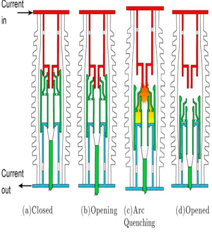
This device is filled with SF6 gas which has very good di-electrical and arc-cooling properties comparing to air. It is compressed and blown in to the arc region. As shown in Fig. 1.1a, when the circuit is closed, the current is carried through the electrodes. When the circuit breaker receives the external opening order, the electrodes separate as shown in Fig. 1.1b. When the electrodes separate as shown in Fig. 1.1c, a plasma formed, and the arc is created. In this situation, the current is still conducted by the ionized gas. Therefore, a high pressure SF6 gas is blown into the nozzle surrounding the arc column in order to cool down the inter-contact region and to extinguish the arc at the next "current zero".

In order to develop and design circuit breakers, an accurate and robust numerical simulation is necessary. For example, General Electric uses the M C3 _{code developed at Ecole} Polytech-nique de Montreal in collaboration with General Electric grid solution. This code has various features that are able to simulate the operating conditions of a circuit breaker accurately. Phenomena occurring in HVCBs are multi-physical, and such numerical simulations are very arduous. In recent HVCBs, the radiant heat emitted by arc ablates the teflon wall whereby the arc energy is used to increase the pressure of the thermal chamber in order to help the SF6 flow in quenching the arc. Thus, the radiant heat transfer plays a very significant role in the HVCB mechanism simulation.

1.2 Physics Inside a HVCB

There are multiple simultaneous physical phenomena occurring in a HVCB. The first and principal is the electrical energy which produces the electrical and magnetic fields which conduct the current through the plasma. The electrical field produces the Joule’s effect (the ohmic heating) and the magnetic field induces the magnetic forces on the electric arc. At the same time, a supersonic flow of SF6 is blown onto the arc and shock waves form. An additional phenomenon that occurs in a HVCB is the radiant heat transfer. When electrodes separate, and the electric arc created produces a high temperature plasma. Hence, a radiant heat transfer occurs between the arc and the walls of the nozzle surrounding the arc. This heat transfer needs to be investigated to better simulate the thermal environment in order to compute the ablation rate of the nozzle wall close to where the arc is located.

The ablation rate is important because of two consequences. First, it is a limiting factor that determines the life time of a HVCB. Second, in the case of a short circuit or overload in the power network, the radiant heat transfer, and consequently, the ablation rate in the HVCB are higher, and the wall ablation builds up the pressure of the chamber favoring the arc quenching. Therefore, the radiant heat transfer should be simulated accurately. Moreover, the simulation should be fast enough in order to make the calculation practical in a design environment.

1.3 Numerical Simulation

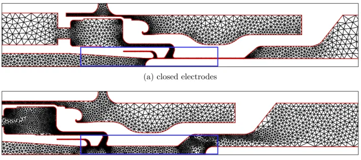
The M C3 software proposes various original feature for modeling arcing-flow in comparison with other CFD codes. The main part of the program is the simulation of the flow where the transient compressible Euler equations are solved. Because of the fast and transient nature of the operation, the viscous terms are not taken into account. The Euler equations are discretized in the time and space using a finite volume axisymmetric formulation. As shown in Fig. 1.2, this discretization is performed on the geometry of a circuit breaker using a triangular unstructured grid. Figure 1.2a shows two closed electrodes in the blue box at time t=9(ms), and Fig. 1.2b presents these electrodes at time t=35(ms) when they are separated and a convergent-divergent nozzle is formed. In order to simulate the flow, the Euler equations are solved explicitly at each time step using a real gas version of the Roe scheme.

1.3.1 Euler Equations

The viscous terms in the Navier-Stokes equation in a circuit breaker are neglected, so the governing equations for fluid dynamics simplify as,

(a) closed electrodes

(b) open electrodes with nozzle

Figure 1.2 A typical circuit breaker geometry with the triangular mesh

∂U ∂t + ∇.F = S (1.1) where            U : conservative variables S : source term vector F : flux matrix

Equation 1.1 states the conservation of mass, the momentum, and energy, and it can be written in conservative form :

U =         ρ ρur ρuz ρe         S =         Sm P/r 0 Se         F =         ρur ρuz ρurur+ P ρuruz ρuruz ρuzuz+ P ρure + P ur ρuze + P uz         (1.2)

These expressions correspond to the axisymmetric configuration where z and r are the axial and radial coordinates, and uz, ur, ρ, and e are the axial and radial velocity, density, and specific energy of fluid, respectively. The specific energy e is the sum of the internal energy of fluid, ei, and the kinetic energy.

where e = ei+ u2

z+ u2r 2

The variables ρ and e are function of temperature, T, and pressure, P. In addition, the equation of state is required,

ρ = ρ(T, P ) e = e(T, P )

(1.3)

These relationships can be determined by expressions for real gases in either single or multiple species [Godin (1999)].

1.3.2 Discretization

By integrating Eq. 1.1 over control volume V , the integral form of Euler equations becomes : ∂ ∂t Z V U dV + I ∂V F.ds = Z V SdV (1.4)

where the second term in the left hand side is obtained from the divergence theorem. The discretized form of these equations are given as Eq. 1.5, where the conservative properties are explicitly computed in each time step.

Un+1_p = Un_p −   ∆t Vp Nsides X k=1 Fn_p,kLp,k  + ∆tSn_p (1.5) where           

Un: conservative variables at nth time step ∆t : time step

Sp : source term vector Vp : volume

k : flux matrix Lp,k: length of side

The discretization element, p, corresponds to a control volume for which the flux balance in each iteration is computed. More details are given by ref. [Godin (1999)].

1.3.3 Source Terms

The source terms vector S including Sm and Seare added to the Euler equations to compute the effect of electric arc on the flow. The final step is to compute ohmic heating, radiative heat transfer, and ablation rate. The mass source term represents the injection of the teflon

vapor inside the cell attached to the teflon wall, Sm = 1 V Nsides X k=1 ˙ mkLk (1.6) ˙ mk =      qk hν

for an ablated side 0 otherwise, where           

V : volume of cell Lk : length of edge

k : kth side qk : incident normal radiative flux ˙

mk: the ablation rate per unit surface unit hν : vaporisation enthalpy per unit mass The vaporization enthalpy for the teflon is known, and the normal incident flux, qk, is com-puted by the P1 or implicit FVM. Therefore, the energy source is a summation of ohmic heating, radiative heat, and ablated vapor injection equation,

Se= Sohm− Srad+ egSm (1.7)

where eg is the energy per unit mass and it is a function of temperature.

where           

Sohm : ohmic source Srad : radiation source Sm :mass source term The ohmic heating is computed by the Joule effect,

Sohm = σE2 (1.8) where    σ : electric conductivity E : electric field

The last term to compute is the radiative energy source term,

Srad = ∇.q = Nbands

X

λ=1

1.3.4 The P1 Model

The P1 model is used in M C3 _{for the simulation of the radiative heat transfer [Eby et al.} (1998)]. Considering the radiant intensity as a function of location and direction in terms of a two-dimensional Fourier series leads to,

∇.( 1 κλ ∇Gλ) = 3κλ(Gλ− 4πIbλ) (1.10) where           

κλ : spectral radiation absorption coefficient in the band λ Gλ : incident radiation in the band λ

Ibλ : the black body intensity emmited in the band λ

To solve Eq. 3.1.3, a proper boundary condition is required.

Boundary conditions    Dirichlet :G =0 M arshak :(1/κ)∇G.ˆn = − (3/2)G

1.3.5 Other Numerical Simulations

In order to simulate moving walls in HVCBs, an ALE formulation is required for the resolution of the gas dynamics equations. In addition, due to a great difference in scale of the various phenomena involved, it is necessary to adapt the mesh dynamically. This characteristic of M C3 _{allows the mesh to be distributed as a function of gradient of variables for an efficient} use of memory and computational time.

1.4 State of The Art, Contributions and Research Objectives

As mentioned in previous sections of this chapter, the radiative heat transfer determines the ablation rate and the pressure build up in the thermal chamber. In addition, the time for calculation is very dependent on the method used for radiative simulations. For example, within a HVCB the arcing simulation time is t=20(ms) and assuming a time step, ∆t = 5 × 10−6, leads to a number of time steps equal to 4 × 106. If the radiative simulations is carried out every 20 time steps, the method of radiation simulation is called 200,000 times. If each simulation takes 1(s), a time of 56(hours) will be needed to complete the computation for simulations of the radiative heat transfer, alone. Therefore, applying an efficient method for simulation of the radiation significantly decreases the total time needed for simulations of a HVCB.

The current simulation software use the P1 model and the implicit finite volume discrete or-dinates method (FVMDOM or FVM) for solving the radiative transfer equations. However, the P1 method is not accurate in some wavelengths for absorption coefficient, but it is com-putationally very fast. The implicit version of the FVM is accurate, yet it is comcom-putationally expensive, and it is not applicable in practice.

The FVM can be accelerated by using an explicit approach and thus avoid solving the equations iteratively. This will require some modifications based on a specific space marching algorithm.

The objective of this project is to improve the computational efficiency of the radiant heat transfer calculation in a HVCB. Specifically, this project aims to improve the finite volume method using a space marching for an explicit solution.

This approach is possible if the circuit breaker is considered as a non-scattering medium and the walls around the arc are non-reflecting.

1.5 Overview of the Thesis Report

This thesis includes five chapters : The first chapter presents an overview of the operation of a HVCB and the physical phenomena involved. In addition to the proposed approach for an efficient solution of the radiative heat transfer, the specific objectives of the project are stated. In the second chapter, the methods that have been used to simulate the radiation in a HVCB are outlined. In the third chapter, the methodology for the finite volume method in an axisymmetric configuration is introduced. Moreover, the explicit solution procedure of the FVM using a marching order map is presented. In chapter four, the results are presented and discussed, followed with a conclusion in the fifth chapter.

CHAPTER 2 LITERATURE REVIEW

2.1 Introduction

The radiative heat transfer plays a significant role in many engineering applications like furnaces and circuit breakers, so having an efficient numerical simulation of the radiation is of interest. In a HVCB the radiation is the principal mechanism of the heat transfer which ablates the nozzle teflon walls and is responsible for the pressure build up that helps to quench the arc. In this chapter, a literature review is conducted to cover some of the numerical methods which have been used to simulate radiative heat transfer in high voltage circuit breakers.

2.2 NEC

In order to compute radiant heat transfer in a plasma media inside a HVCB, a model based on the net emission coefficient (NEC) was proposed by Lowke (1974), Lowke (1978), Aubrecht and Lowke (1994), and Gleizes et al. (1991). The model for radiation transfer predicts that the arc diameter is proportional to the square root of the current and the arc voltage. This model also states that temperature is independent of current. However, this method only gives an approximation of the net radiation which leaves the hot plasma region and does not simulate accurately the strong self-absorption of the spectrum at the cold boundary of the arc. In fact, this method gives reasonable results when the optical thickness of the medium is thin and the flux on the boundary is not of interest. Thus, this method calculates reasonably well the radiative flux in the arc core, but it is not able to give the precise results for the flux on the nozzle wall which is critical in computing the ablation rate in the circuit breakers [Nordborg and Iordanidis (2008)].

2.3 The P1 Method

Instead of solving the radiative transfer equation (RTE), the P1 method proposed by Jeans (1917), uses a decomposition of direction and space in form of a Fourier function for radiant intensity that results in a Helmholtz type equation. To overcome the NEC drawbacks, the P1 was implemented in order to simulate the radiation in a Euler arc-flow solver by Eby et al. (1998). They compared the P1 with NEC and applied it to a high-voltage SF6 circuit-breaker simulator. It was thus concluded that unlike the NEC method, the P1 is capable of

computing the strong self-absorption rate at the arc boundary and it is more accurate as it avoids some overheads because of the evaluation of net emission and power loss factors. The P1 method was applied to compute the ablation on the walls [Godin et al. (2000)] giving an improvement over the NEC. However, it does not give accurate results in particular radiation bands when the optical thickness is thin. Furthermore, the method is unable to capture the axial variation of the flux which is consequent on geometry. In addition, the results obtained from the P1 show various non-physical behaviors for this method in computing circuit breaker configurations [Melot et al. (2012)].

2.4 Discrete Ordinates Method

Another method named discrete ordinates method (DOM) was proposed by Chandrasekhar (1960) developed by Lathrop (1966), to study the transport of neutrons. However, it was practically inapplicable at the time because of the lack of CPU power. According to the method, the radiative transfer equation is discretized in space using a spatial grid and is discretized in angular space by choosing an arbitrary quadrature. The DOM was only used in the 1980s by pioneers like Fiveland (1988) for calculation of the radiative transfer. Recently, this method was tested by Nordborg and Iordanidis (2008) and Iordanidis and Franck (2008) in order to resolve the RTE in the HVCB simulation. They compared the DOM with the P1 in arc simulation and concluded that the DOM is more accurate, while the P1 is faster. Raithby (1999) states that the DOM cannot satisfy radiant energy conservation where the geometry wall normal vectors are not directed along the Cartesian axes. Moreover, the DOM is not flexible in selecting the angular discretization.

2.5 The Finite Volume Method

As a consequence of the shortcomings of the NEC, P1, and DO methods, the finite volume method (FVM) was developed. In the FVM proposed by Raithby and Chui (1990), to ensure the conservation of energy, the spatial and the angular domains both are arbitrarily subdivi-ded into control volumes and control angles, respectively. Raithby’s method was developed using the control volume finite volume grid as described by Baliga and Patankar (1983). However, Raithby used a somehow complicated formulation using a high-order spatial diffe-rencing scheme. Thus, a simpler formulation was proposed by (Chai et al., 1994) in which an exponential scheme is used to solve the RTE. The FVM leads to a system of equation which can be solved either implicitly and explicitly when the medium is non-scattering, but a specific order is needed for nodes in order to solve the equations explicitly. Chai et al.

(1994), Raithby and Chui (1990), and Kim (2008) have used the explicit solution procedure for the structured grid and an unstructured mesh is used by Murthy and Mathur (1998) to solve implicitly the RTE. Moreover, Chui and Raithby (1993) proposed a method to resolve the RTE on a non-orthogonal grid in order to simulate the radiation in complex geometries. An intelligent procedure was proposed by Chui et al. (1992) in order to compute the radiant heat transfer in two-dimensional axisymmetric configurations on structured grids. The me-thod uses a three-dimensional spatial and an angular discretization to solve the RTE in an axisymmetric geometry. A similar mapping is used by Murthy and Mathur (1998) to com-pute implicitly the radiative heat transfer on unstructured grid for axisymmetric geometries. Due to this great versatility, the FVM has been used in several commercial software such as FLUENT. The FVM is used by Melot et al. (2012) in order to simulate the radiant heat transfer in the HVCB using a method very similar to Murthy and Mathur (1998) method. Ho-wever, an explicit and computationally more efficient solution is possible for a non-scattering medium when the walls are assumed as a black body. Consequently, in the present work the RTE is resolved explicitly without any iterative process using a marching order map similar to the method given by Kim (2008).

2.6 Hybrid method

According to inaccurate results of the P1 in low optical thickness and the expensive compu-tational costs of the FVM which is very important in simulation of physics in the HVCB a hybrid method was proposed by Reichert et al. (2012). They used FLUENT which solves the RTE with a implicit version of the FVM. The Hybrid method uses the P1 in high optical thicknesses where the P1 results are reasonable and employs the FVM proposed by Murthy and Mathur (1998) for the optical thickness lower than a specific value. However, in the present work although the FVM is only used for the RTE on a Cartesian grid, the explicit solution of final equations makes it computationally inexpensive. Consequently, with this explicit solution of the FVM the results obtained are accurate and the method is reasonably fast.

2.7 Conclusion

After reviewing the literature, the FVM has been shown to be the most appropriate method to simulate the radiative heat transfer in the HVCB in terms of accuracy. This method uses both spatial and angular discretizations. Assuming wall of the nozzle surrounding the electrical arc in the circuit breaker as a black body, an explicit numerical solution can be

CHAPTER 3 THE FINITE VOLUME METHOD IN AXISYMMETRIC CONFIGURATIONS

As mentioned in Chapter 2, the finite volume method was proposed by Raithby and Chui (1990) and since then, it has been implemented by many researchers in the various engineering applications. In this chapter, the finite volume method is briefly presented. The radiative transfer equation for axisymmetric configurations is then introduced, and an explicit method is presented for the solution of the RTE, explicitly.

3.1 Finite Volume Method 3.1.1 Overview

The basic approach of the FVM is to discretize the radiant intensity within the solution domain using spatial non-overlapping control volumes surrounding nodal points on which the radiant intensity will be determined. Furthermore, the angular spherical domain is divided into non-overlapping control angles ωl _{which shows the directional dependence of the radiant} intensity.

3.1.2 Radiative Transfer Equation The main objective of the FVM is to obtain Il

P which is the radiant intensity on the node P in the direction l. Therefore, a set of algebraic equations should be formed in order to obtain the unknown I_Pl, and an algorithm is used to solve these equations. The set of equations for I_Pl is determined by governing equation for radiative heat transfer. As illustrated in Fig. 3.1, the radiative transfer Eq. 3.1 states the rate of change of intensity I( ~R, ~S) at specific spatial location ~R through the path length of ds in the direction of ~s is :

dI

dS = −(κa+ σs)I + κaIb+ σsI (3.1) The RTE, Eq. 3.1, expresses the energy conservation over a control volume through the direction ~S. The FVM proposes a way to solve this equation for a control volume. Thus Eq. 3.1 should be discretized in both, the spatial space, and the angular space.

ds

Figure 3.1 Radiation energy balance

performing the integration over control volume dV and control angle dω gives,

Z Af Z ωlI l_{( ~S. ~n} f)dωdAf = Z Vp Z ωl[−(κa+ σs)I + κaIb + σsI]dωdV (3.2)

where ~nf is the unit outward normal vector of surface f , while VP and Af are the area of surface f and volume of control volume, respectively. Equation 3.2 states the energy balance between radiant energy leaving from control volume and the net radiant energy generated inside the control volume due to emission, scattering, absorption, and in-scattering. If all the variables in right hand side of Eq. 3.2 are assumed to be constant over volume VP and solid angle ωl_{, it becomes :} Z Vp Z ωl[−(κa+ σs)I + κaIb+ σsI]dωdV ≈ [−(κa+ σs)IP + κaIb+ σsI]ωlVp (3.3)

Z Af Z ωlI l_{( ~S. ~n} f)dωdAf = Nsurf aces X f =1 Af[ Z ωlI l f( ~S. ~nf)dω] (3.4)

where If is the intensity value on the surface f and it should be evaluated in terms of the nodal value of the intensity IP.

3.1.3 The axisymmetric RTE

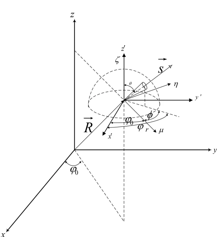
In order to solve the RTE for axisymmetric geometries, it is written in cylindrical coordinate system (Fig. 3.2). 1 r ∂ ∂r[µrI(~r, ~s)] + 1 r ∂ ∂ϕ0 [ηI(~r, ~s)]+ ∂ ∂z[ξI(~r, ~s)] − 1 r ∂ ∂φ[ηI(~r, ~s)] = −β(~r)I(~r, ~s) + κa(~r)Ib(~r) + σs(~r) 4π Z Ω0_=4πI(~r.~s 0 )dΩ0 (3.5) where                  µ = sinθcosφ η = sinθsinφ ξ = cosθ β(~r) = κa(~r) + σs(~r)

are the cosines of the path, ~s, in x, y, z directions and the extinction coefficient of the participating medium, respectively. The intensity is function of 2-spatial and 2-angular co-ordinates, I(r, z, θ, φ). However, for an axisymmetric configuration the term ∂

∂ϕ0 = 0 and Eq. 3.5 reduces to : 1 r ∂ ∂r[µrI( ~R, ~S)] + ∂ ∂z[ξI( ~R, ~S)]− 1 r ∂ ∂φ[ηI( ~R, ~S)] = −κa( ~R)I( ~R, ~S) + κaIb( ~R) + σs(~r) 4π Z Ω0_=4πI( ~R.~s 0 )dΩ0 (3.6) Assuming a non-scattering medium for the HVCB, the final form of the RTE in axisymmetric



R



s



x

r



0





z

z

0



x

y

y 

form becomes,

dI( ~R, ~S)

ds = −κaI( ~R, ~S) + κaI( ~R) (3.7) In this analysis, all boundaries can be assumed diffuse-gray where the RTE is subject to the following boundary condition for the intensity on the wall Iw :

Iw(Rw, ~S) = εwIb(Rw) + 1 − εw π Z ~ nw.~s0<0 I(rw, ~s0)dω0 (3.8)

In a circuit breaker, all boundaries are assumed as black body (εwall = 1), so for a surface with a specific temperature (TB), the boundary condition is,

Iw(Rw, ~S) = σBTB4/π (3.9)

3.1.4 Finite Volume Method for Axisymmetric Configurations

The finite volume method(FVM) enforces the conservation laws for discrete volumes (com-putational mesh) to solve the governing equations in fluid dynamics and heat transfer si-mulation. Equation 3.6 states the conservation of radiant energy in a specific direction over a differential control volume and within an infinitesimal control angle in an axisymmetric configuration.

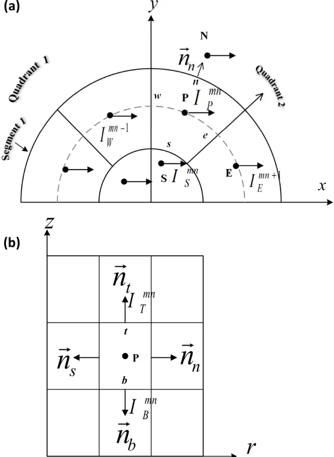
To solve this equation, the computational domain is discretized as shown in Fig. 3.3 for a cylindrical domain. The intensity is located on the nodal points P, E, W, S, N, T, and B. Each nodal point P is enclosed by six control surfaces identified by e, w, s, n, t, and b. Furthermore, the angular space is divided into discrete solid angles ωmn _{that are defined for} mth polar and nth azimuthal solid angles in a range of φn−1/2 _{to φ}n+1/2 _{and θ}m−1/2 _{to θ}m+1/2 as shown in Fig. 3.4. The integration points are located on the surfaces of the control volume (Kim, 2008). Eq. 3.7 is integrated over a control volume, VP, and a control angle ωmn to obtain the discretized form of the RTE :

6 X i=n,s,t,b,w AiDmni I mn i = [−κa,PIPmn+ κa,PIb,P]ωmnVP (3.10) where Ai is the control surface area and Ib is the black body intensity which is determined

N

P

S

E

e

n

w

s

t

b

z

y

t

n

r

n

n

r

s

n

r

b

n

r

1

−

mn

W

I

1

+

mn

E

I

mn

S

I

mn

P

I

n

n

r

r

(a)

(b)

mn

T

I

mn

B

I

P

x

Figure 3.3 The control Volume in a cylindrical enclosure around node P and molecule of nodal points as given by Kim (2008) :(a)top view (b)side view

z

e

r

2

/

1

+

m

θ

2

/

1

−

m

θ

θ

(a)

φ

ω

n

φ

1

+

n

φ

2

/

1

+

n

φ

r

e

r

(b)

Figure 3.4 The angular discretization as given by Kim (2008) :(a)azimuthal direction (b)polar direction

with domain temperature and : Dmn_f = Z ωl(~s. ~nf)dω (3.11) where D_nmn= −Dmn_s = Z φn+1/2 φn−1/2 cosφdφ Z θm+1/2 θm−1/2 sin 2_{θdθ (3.12a)} Dmn_t = −Dmn_b = Z φn+1/2 φn−1/2 dφ Z θm+1/2 θm−1/2 sinθcosθdθ (3.12b) D_nmn= −Dmn_s = Z φn+1/2 φn−1/2 cosφdφ Z θm+1/2 θm−1/2 sin 2_{θdθ (3.12c)} D_emn+1/2 = Z φn+1 φn sinφdφ Z θm+1/2 θm−1/2 sin 2 θdθ (3.12d) Dmn−1/2_w = Z φn φn−1sinφdφ Z θm+1/2 θm−1/2 sin 2_{θdθ (3.12e)} and, At= Ab = sin( 1 2∆ϕ0) × (rn+ rs) × cos( 1 2∆ϕ0) × (rn− rs) (3.13a) Ae = Aw = (zt− zb) × (rn− rs) (3.13b) As = 2 × rs× sin( 1 2∆ϕ0) × (zt− zb) (3.13c) An = 2 × rn× sin( 1 2∆ϕ0) × (zt− zb) (3.13d) where, rf and zf are the (r, z) coordinates for center point of the f surface and ∆ϕ0 is the angular increment, respectively.

3.1.5 Evaluating the Intensity on the Control Surfaces

In circuit breaker simulation, both the RTE and the gas dynamics equations are solved on the same grid and due to the presence of high gradient in the flow, this grid is very fine in order to have accurate results. Consequently, a first order scheme on such a fine grid can be used to evaluate the intensity on surfaces of the control volume, Ib,e,n,s,t,w. In each direction, for the surfaces which are located upstream of the node P, the intensity on the surface is

considered as I_Pmn and for the surfaces which are downstream of the node P the intensity of nodes are : I_i=n,t,emn = I_Pmn (3.14a) I_smn = I_Smn (3.14b) I_wmn−1/2 = I_Wmn−1 (3.14c) I_bmn = I_Bmn (3.14d)

Where IB,E,N,S,T,P are nodal values of the intensity.

3.1.6 Final Form of the Equations

Replacing the value of the intensity in Eq. 3.10, the final form of the equations for the radiant intensity on node P is :

amn_p I_pmn = X I=N,S,T,B,W

a_II_Imn+ bmn_{P (3.15)}

To solve this equation explicitly an appropriate marching order is necessary.

3.1.7 Axisymmetric Extension

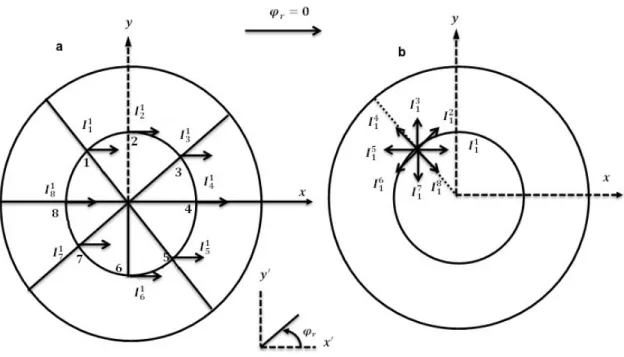
The radiant heat transfer is axisymmetric when the intensity does not depend on ϕ0 and the intensity is indicated as I(r, z, φ, θ). The intensities shown in Fig. 3.5a are located in the same r, z, and θ. The spatial angular difference ∆ϕ0 for all points (i=1,2..., 8) is π/4. The points (i=1,2..., 8) are located at ϕ0 = 7π/8, 5π/8, 3π/8, ... respectively, and the angle φr = 0. Thus, the angle φ = ϕr− ϕ0 is −7π/8, −5π/8, −3π/8, ... for the intensities I11, I21, I31, .... However, in Fig. 3.5b the intensities are located at same r,z, and θ and at spatial angle ϕ0 = 7π/8, with angular azimuthal angle ϕ0 = 0, π/4, π/2, ... for the intensities I12, I12, I12, ... , respectively and the φ = 7π/8, −5π/8, −3π/8, ... (∆ϕ0 = ∆φ). Therefore, r,z, φ, and θ are the same for I1m and I1

m in Fig. 3.5a and Fig. 3.5b. Due to this mapping between intensities in Fig. 3.5a and Fig. 3.5b, it is more convenient to solve the domain in Fig. 3.5a to obtain the intensity for each node.

Figure 3.5 A mapping between the distribution of intensity in cylindrical coordinate system and intensity at specific point in all directions

3.1.8 Solution Procedure

In order to solve Eq. 3.15 explicitly for Imn

p , a marching order for nodes is employed. For θ < π/2 and ϕ0 > π/2 the marching order is from outer wall to the center point for each z level and it is repeated from bottom to the top of the cylinder for other z levels. At each node the radiant intensity is computed using the intensities which are computed in upstream direction of that node. For example, for a small grid shown in Fig. 3.6 in segment 1 where ϕ0 > π/2, the marching order is the node on the wall → a → b, the node on the wall → d → e and finally the node on the wall → g → h . As soon as, the marching of all the nodes is finished in the quadrant 1 and the intensity is computed for each nodes the same procedure is carried out for the nodes in the quadrant 2 where ϕ0 < π/2. However, in this quadrant for each segment the marching is from center to the wall. For θ > π/2 the same marching order for nodes is considered, but moving in the z direction is from the top to the bottom. The nodal intensity is obtained explicitly for a given medium temperature if the enclosure walls are assumed black bodies.

z

r



z

e

a

b

d

e

g

_h

x

a

b

0



Figure 3.6 A marching order map given for a small grid

3.2 The Flux and the Incident Radiation

Using the solution procedure for the RTE, the nodal value of the radiant intensity is obtained, by which the radiant heat flux q is computed. Since the ablation rate in the HVCB plays a significant role and it is function of the flux on the Teflon walls, and also the thermal energy

of plasma includes the radiation source term, the flux (qλ), the spectral incident radiation (Gλ), and consequently, the radiation source term (∇.q) are computed :

qλ = Z ωlIλ( ~R, ~S) ~Sdω (3.16) Gλ = Z ωlIλ( ~R, ~S)dω (3.17) ∇.qλ = κλ(4πIλb− Gλ) (3.18)

Equations 3.16, 3.17, and 3.18 show the dependence of the absorption coefficient on the wavelength of radiation.

3.3 Spectral Characteristics of Radiation

All the values obtained in the previous section have wavelength dependence, so they should be integrated over the spectrum to acquire the total values. However, due to the large number of wavelengths for absorption coefficient of gas in a circuit breaker a continuous integration over the spectrum is not possible, and therefore, the spectrum is divided by a few bands. As given in Eq. 3.19, the result for each band are separately calculated and a summation over all bands is performed to obtain the total value :

G = Nband X i=1 Gi q = Nband X i=1 gi ∇.q = Nband X i=1 ∇.qi (3.19)

3.4 Other Physical Phenomena

In order to simulate the radiative heat transfer in a certain time, the equations of other physical phenomena should be previously solved. As given in Section 1.3, the compressible Euler equation coupled with the equation of electrical conservation is being solved. Since all the phenomena are transient, the thermal quantities required for simulation of radiative heat transfer are obtained at a certain time step. The source term obtained from simulation of the radiation will be used in the next time step.

CHAPTER 4 RESULTS AND DISCUSSION

4.1 Introduction

In this chapter, the finite volume method presented in Chapter 3 is applied to solve the RTE in non-scattering media using an explicit scheme. Firstly, this method is utilized to compute the radiant flux on the wall of a cylinder for various optical thicknesses and the results are compared with an analytical solution. Secondly, the method is employed to simulate the radiant heat transfer within a geometry similar to a circuit breaker ; these results are then compared with results of the P1 method and FVM obtained from the M C3_{. Finally,} the method is utilized to simulate radiative heat transfer in the Lewis nozzle which is a benchmark test case in validations in circuit breaker simulations. The results of present work are compared with the P1 results obtained from the M C3.

4.2 Isothermal Cylinder

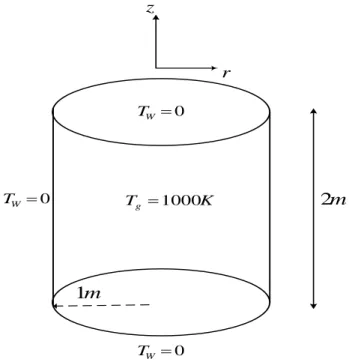
The classical isothermal cylinder is used for first validation case. The cylinder has a 1(m) radius and a length of 2(m) as shown in Fig. 4.1. The temperature in the participating medium is 1000K, and it is fixed at T=0K for the cylindrical wall and both ends of the cylinder.

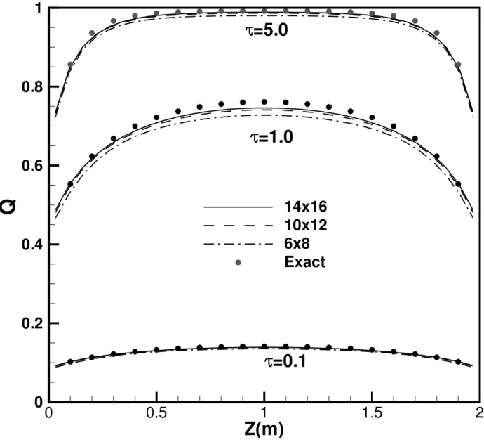
Figure 4.2 shows the normalized radiative flux (Q∗ = Qr/σT4) on the cylindrical wall for three different values of the optical thickness, defined as τ = rκa where Qr, σ, T, κa, and r are radial flux, Stefan-Boltzman coefficient, medium temperature, absorption coefficient, and radius of the cylinder, respectively. First, the results are compared for two Cartesian grids, Nr × Nz = 17×33 and 50×75 grid points where Nr and Nz are number of grid points in radial and axial directions, respectively. For both cases, the discretization of angular space is Nφ× Nθ = 14×16 where Nφ and Nθ are the number of divisions in the azimuthal and polar directions, respectively. The results are compared to the analytical solution from [Dua and Cheng (1975)]. Globally, the analytical results confirm the results of present work even on coarse grids.

Figure 4.3 shows the effect of angular refinement for the same cylindrical case, in Nr× Nz = 17×33. One can see that the angular discretization using Nφ× Nθ = 10×12 directions provides almost the same result as a Nφ× Nθ = 14×16 angular grid. Since the computational time increases linearly with the number of directions, the next results will be computed using a Nφ× Nθ = 10×10 angular discretization.

K Tg 1000 0  W T 0  W T 0  W T m 1 m 2 z r

Figure 4.1 Cylindrical medium with constant temperature

4.3 Semi-Industrial Test Case

Figure 4.4 illustrates the second geometry used to test the current explicit solution scheme. The geometry contains some elements found in circuit-breakers to assess the capability of of the method. As seen in Fig. 4.4, a hot region is placed on the axis with a temperature of Th=1000K. Two blocking regions are inserted into the domain, representing the teflon parts in circuit-breakers. The rest of the domain contains a gas at T=0K with a constant absorption coefficient.

Figures 4.7, 4.8 and 4.9 shows a comparison of the normalized radiative heat flux (Q∗ = Qr/σTh4) on the upper boundary obtained with various methods in the various optical thi-cknesses (τ = .01, 1, 10). The FVM-M C3 _{method is described in Ref. [Melot et al. (2012)].} It implements an implicit version of the FVM method from the solution of the RTE. The P1-M C3 method is described in Ref. [Eby et al. (1998)] and it implements the classical P1 method. Both methods are compared to the present work for three different values of the absorption coefficient. The FVM-M C3 _{and the P1-M C}3 _{method are computed on a} triangu-lar grid composed of 20780 nodes shown in Fig. 4.5 using Nφ× Nθ = 10×10 directions. The present method uses a 20700 nodes Cartesian grid shown in Fig. 4.6 and Nφ× Nθ = 10×10 directions. Firstly, one can observe in Fig. 4.7,4.8, and 4.9 that both FVM methods produce similar results. Minor differences can be attributed to the different grids used. Secondly, the

Z(m)

Q

*

Figure 4.2 The radiative heat flux on the cylinder wall in various spatial grids and Nφ× Nθ = 14×16

results confirm the poor performance of the P1 method for such cases, especially for low and high coefficients of absorption and for long distance propagation of radiation over an obstacle in the domain.

Unlike the FVM, the P1 model is an elliptic method which cannot accurately model the directional variation of the radiant intensity. Therefore, as shown in Fig. 4.7, 4.8, and 4.9, the P1 gives a very smooth results without capturing the presence of obstacles in the domain. However, the FVM not only gives the results showing the variation of temperature in the domain, but also is able to handle the presence of the obstacles in the domain. Since in this test case the absorption coefficient is constant across the domain, not only the absorption in cold part, but also the emission from the hot region is function of this coefficient. Therefore, as shown in Fig. 4.7, the flux on the upper boundary is the optical thickness is τ = 0.1 is low because the emission is low. Similarly, as shown in Fig. 4.9 for a high optical thickness

Z(m)

0

0.5

1

1.5

2

0

0.2

0.4

0.6

0.8

1

14x16

10x12

6x8

Exact

=0.1

=5.0

=1.0

Q

Figure 4.3 The comparison of the radiative heat flux obtained with numerical simulation on the cylinder wall in various angular grids and Nr× Nz = 17×33

τ = 5.0, although the emission is higher, the cold domain absorbs the energy and does not allow it to reach the boundary, and the flux is low. Thus, as plotted in Fig. 4.7 the maximum value of flux is for the case with medium optical thickness τ = 1.0 where there is a compromise between the low emission from hot region and low absorption by cold region. It can be concluded that solving an elliptic equation using the P1 method, makes it inaccurate for predicting the radiant heat transfer when the medium is optically thin or direction of emission is considerably important.

2 1.2 0.2 0.3 0.2 0.3 0.9 0.1 .2 Hot Region Z R

Figure 4.4 Semi-industrial test case Geometry

Z(mm)

r(m

m

)

0

500

1000

1500

2000

0

200

400

600

800

1000

Z(mm)

r(m

m

)

0

500

1000

1500

2000

0

200

400

600

800

1000

Figure 4.6 Cartesian grid used for semi-industrial test case Geometry.

Z(M) 0 0.5 1 1.5 2 0 5E-05 0.0001 0.00015 0.0002 0.00025 0.0003 0.00035 0.0004 0.00045 0.0005 0.00055 FVM-MC3 PRESESNT WORK P1-MC3

Q

Figure 4.7 Comparison of the radiative heat flux obtained with current numerical method and results obtained with M C3 _{for κ = 0.1m}−1

4.3.1 CPU Time

Table 4.1 summarizes the CPU time for the radiation computation for the semi-industrial case. It can be observed that on a Nφ × Nθ = 10×10 angular discretization, the present

Z(M) 0 0.5 1 1.5 2 0 0.0005 0.001 0.0015 0.002 FVM-MC3 Present work P1-MC3 m-1

Q

Figure 4.8 Comparison of the radiative heat flux obtained with current numerical method and results obtained with M C3 for κ = 1.0m−1

Z(m) 0 0.5 1 1.5 2 0 5E-05 0.0001 0.00015 0.0002 FVM-MC3 PRESENT WORK P1-MC3 = 5.00m-1

Q

Figure 4.9 Comparison of the radiative heat flux obtained with current numerical method and results obtained with M C3 _{for κ = 5.0m}−1

method is more than 50 times faster than the previous FVM-M C3. Also, the computation time is closer to that of the current implementation of the P1 model. This result confirms a very high potential of the method in reducing computation time for simulation of radiation in the circuit breaker.

FVM-M C3 _{P1-M C}3 _{Present Method}

40 sec .03 sec .7sec

Table 4.1 Comparison of CPU time

4.4 Circuit Breaker Model

The present model is applied to a circuit breaker model filled with SF6, in order to simulate radiation heat transfer. As shown in Fig. 4.10 and Fig. 4.11, the computational domain is a convergent-divergent nozzle with 2 electrodes located at two ends. The flow enters the nozzle from the inlet on the left, and after passing over electrodes and forming arc, exits from the right outlet. Since all this physical phenomena are transient, transient Euler, magnetic, and electrical equations are solved. However, in order to solve the RTE at a given time only, temperature and pressure fields at that time are needed. Figure 4.14 shows the temperature field for SF6 obtained in a circuit breaker model at t = 8(ms), using M C3 and the P1 radiation model. It shows the hot region containing the electrical arc between 2 electrodes from which the radiant heat is emitted through the medium and impinged to the nozzle wall. Moreover, Fig 4.13 shows the variation of absorption coefficient with temperature for band number five. This dependency will be discussed in the next section.

Z(mm) -100 -50 0 50 100 150 0 20 40 Teflon Electrode Electrode Outlet Inlet

Figure 4.10 The nozzle inlet outlet

Computations are performed on a Cartesian and triangular spatial grid composed of about 20000, as shown Fig. 4.12 and Fig. 4.11, respectively, where Nφ× Nθ = 10×10 directions are used as the angular mesh. Due to axisymmetry, half of the geometry is utilized.

Z(mm)

r(m

m

)

Figure 4.11 The nozzle geometry and the Cartesian computational grid

Z(mm)

r(m

m

)

Figure 4.12 The nozzle geometry and the tri-angular computational grid

Z(mm)

r(m

m

)

Figure 4.13 Absorption coefficient field for band number 5

4.4.1 Spectral Emission

Fig. 4.15 shows that the absorption coefficient of plasma SF6 at a certain temperature and pressure is a function of the emission frequency. However, the exact radiative heat trans-fer computation in a circuit breaker using a continuous spectral distribution is practically impossible.

Figure 4.14 Temperature field for the arc happening between 2 electrodes

Figure 4.15 Continues absorption coefficient of SF6 VS. frequency in the atmospheric pressure [Randrianandraina et al. (2011)]

Figure 4.16 demonstrates that the total spectrum is subdivided into 7 intervals (called bands) in which for a given temperature, the absorption coefficient is constant and the plasma can be assumed as a gray body. Moreover, Fig. 4.17 displays the mild variation of the absorption coefficient with temperature for two methods of averaging presented in ref.

[Randrianan-Figure 4.16 Mean SF6 absorption coefficient VS. frequency in the atmospheric pressure [Ran-drianandraina et al. (2011)]

Figure 4.17 Mean SF6 absorption coefficient VS. frequency in the atmospheric pressure [Ran-drianandraina et al. (2011)]

draina et al. (2011)]. Consequently, the computation is limited to the small number of bands, and then a summation over the bands which allows to calculate the radiative heat transfer inexpensively while results are reasonably correct.

4.4.2 Flux on the Wall

Z(mm)

Q

(W

/m

m

m

)

Figure 4.18 Comparison of the radial radiative heat flux obtained with current numerical method and results obtained with P 1 − M C3 _{for 2 boundary conditions}

Figure 4.18 shows a comparison between the present FVM and the P1 for the heat flux incident on the nozzle wall which is used to calculate the ablation of teflon. It is observed that the value of flux is very low at the beginning and the end of the nozzle where the temperature is low, and it increases between electrodes with a maximum value on the throat where the arc is hottest. The trend of flux value for the FVM and the P1 with Dirichlet boundary condition are in a good agreement. However, the flux value obtained on the throat wall is smoother and more realistic than that obtained by the P1 because the FVM can simulate the radiant intensity in all directions.

The Marshak boundary condition for the P1, that simulates a situation with a convective flow on the boundary, predicts a constant heat flux on the wall which is not physically realistic. However, as seen in Table 4.2, the radiant heat impinging on the nozzle wall achieved from P1-Marshak is relatively closer to value of flux given by the FVM than to that obtained

Z(mm)

Q

(W

/m

m

)

Figure 4.19 Comparison of the radiative heat flux obtained with current numerical method and results obtained with P 1 − M C3 _{for band number 4}

from P1-Dirichlet. Therefore, the P1-Marshak is still reliable although it cannot determine the location of maximum flux.

FVM- Present Work P1-Dirichlet P1-Marshak

15.0M W 9.5 M W 14.4M W

Table 4.2 Comparison of P1 boundary conditions for radiation heat value on the nozzle wall

Moving from the throat to the end of nozzle, the flux obtained from the FVM is slightly higher than that obtained from the P1. In order to analyze this discrepancy, flux on the wall of nozzle is computed by the P1 and FVM for each band separately. It is thus observed that incident radiative flux on the wall emitted in the three first bands is negligible and the radiation impinging on wall is mostly emitted in the band number 4 and band number 5. As shown in Fig. 4.19, the flux obtained from both methods is in relatively good agreement while the FVM gives more realistic results on the throat. The small discrepancies come from

Z(mm)

Q

(W

/m

m

)

Figure 4.20 Comparison of the radiative heat flux obtained with current numerical method and results obtained with P 1 − M C3 _{for band number 5}

the performance of each method which was studied in Sec. 4.3 for the semi-industrial test case.

4.4.3 CPU Time

Table 4.3 gives the CPU time for the radiation simulation of the circuit breaker model case. It can be observed that for about 20000 grid nodes and the Nφ× Nθ = 10×10, the P1 method is 17 times faster than the present model, while the present model is more accurate.

P1-M C3 _{Present Method} .21 sec 3.50sec

4.4.4 Radiation Source Term

The gradient of flux, (∇.q), which is used in the energy source term in the Euler equations, is computed for the circuit breaker for both the P1 model and FVM. As shown in Fig. 4.21 at the boundary of the arc there is a strong self absorption which is displayed in red and orange on the contours. This self-absorption happens in the region that temperature, and consequently, black body emission due to the longer distance from the arc is low and the absorption is high. Both models predicts the self-absorption at the same place, while the P1 predicts a wider area for the self-absorption. Hence, solving the Euler equations using different radiative heat transfer simulation method might give different thermal fields. In Section 4.4.2 the incident flux on the wall of the nozzle for 5 bands were separately studied. It was shown that the 3 first bands do not participate in the flux received by the wall. However, the participation of the 5 bands in the radiative energy source term should also be investigated. As shown in Fig. 4.22 and 4.26, value of the source term in bands 1 and 5 is low. However, as Fig. 4.22a shows the P1 predicts a region with absorption of energy above the arc location. Additionally, Fig. 4.26 shows the contour of radiant energy source term for the P1 matches that for the FVM in the band 5. Figure 4.23 shows that the emission in the band 2 from the core of the arc is very high and there are regions of absorption at the boundary of the arc. In addition, the contours obtained from the P1 and FVM are in a relatively good agreement in this band. However, Fig. 4.23b captures variation of energy in the arc core for the FVM more than that for the P1. Figures 4.24 shows that except a very small region at the arc boundary where the radiative energy is absorbed, in other regions it is being emitted in the band 3. Furthermore, Fig. 4.24b shows that the variation of the emission form the arc core obtained from the FVM is more than that for the P1. The trend of the radiative energy source term for both methods in the band 3 are in comparatively good agreement.

4.5 Discussion

The explicit FVM method is employed to simulate heat transfer in a cylindrical medium with constant temperature at walls. The obtained results from the present work are in a good agreement with the analytic results. Furthermore, the explicit FVM method is exploited in order to simulate radiative heat transfer in a geometry representing an industrial circuit breaker and the results obtained from the present work reasonably match with those obtained from implicit FVM, while the CPU time for the explicit FVM is much less than that for implicit one. Finally, the present method is utilized to simulate radiation in a circuit breaker

(a) Obtained from the P 1 − M C3

(b) Obtained from The FVM

Figure 4.21 Total radiative energy source term contour

model filled with SF6 for which the spectral absorption coefficient is considered in five bands. The results achieved from the present work are compared with those from the P1 method. The incident flux on the wall of the nozzle for first 3 bands are very low while the participation of bands 2 and 3 in the value of the radiative energy source term is not negligible. It is predicted that in some bands P1 can be used while in other bands the FVM must be used to obtain more accurate results.

Z(mm)

-100

-50

0

50

100

150

0

20

40

(a) Obtained from the P 1 − M C3

Z(mm)

-100

-50

0

50

100

150

0

20

40

(b) Obtained from the FVM

Z(mm)

-100

-50

0

50

100

150

0

20

40

(a) Obtained from the P 1 − M C3

Z(mm)

-100

-50

0

50

100

150

0

20

40

(b) Obtained from the FVM