HAL Id: hal-00772163
https://hal.archives-ouvertes.fr/hal-00772163
Submitted on 11 Jan 2021
HAL is a multi-disciplinary open access
archive for the deposit and dissemination of
sci-entific research documents, whether they are
pub-lished or not. The documents may come from
teaching and research institutions in France or
abroad, or from public or private research centers.
L’archive ouverte pluridisciplinaire HAL, est
destinée au dépôt et à la diffusion de documents
scientifiques de niveau recherche, publiés ou non,
émanant des établissements d’enseignement et de
recherche français ou étrangers, des laboratoires
publics ou privés.
Seasonal sea surface height variability in the North
Atlantic Ocean
Nicolas Ferry, Gilles Reverdin, Andreas Oschlies
To cite this version:
Nicolas Ferry, Gilles Reverdin, Andreas Oschlies. Seasonal sea surface height variability in the North
Atlantic Ocean. Journal of Geophysical Research, American Geophysical Union, 2000, 105,
pp.6307-6326. �10.1029/1999JC900296�. �hal-00772163�
JOURNAL OF GEOPHYSICAL RESEARCH, VOL. 105, NO. C3, PAGES 6307-6326, MARCH 15, 2000
Seasonal sea surface height variability in the North
Atlantic
Ocean
Nicolas
Ferry
1 and Gilles Reverdin
LEGOS, Toulouse, France
Andreas Oschlies
Institut flit Meereskunde an der Universit3t Kiel, Kiel, Germany
Abstract. We investigate the seasonal sea surface height (SSH) variability on large spatial scales in the North Atlantic by using both a numerical simulation and in situ data. First, an ocean general circulation model is run with daily forcing from the European Centre for Medium-Range Weather Forecasts reanalysis. We evaluate the different contributions to the seasonal SSH variability resulting from the surface heat fluxes, advection, salt content variability, deep ocean steric changes, and bottom pressure variability. These terms are compared with estimates from in situ
data.
North
of 20øN,
there
is an approximate
balance
between
hQ,
the
air-sea
heat
flux
induced
changes in steric height, and SSH variability. The next important component is the advection (its contribution to the annual amplitude is of the order of 1 cm except near the western boundary); other contributions are found to be smaller. Between 10øN and 10øS the advection variability induced by the seasonal wind stress cycle is the primary source of SSH variability. We then compare the sea surface height annual harmonic from TOPEX/Poseidon altimetry with the steric effect from the heat flux and with model and/or in situ estimates of the other terms. In many areas north of 20øN the balance between h and the altimetric SSH seasonal Q cycle is closed within the
uncertainty
limit of each
of the terms
of the SSH
budget.
However,
h o and
the SSH
do not balance
each
other
in the eastern
North
Atlantic,
and
the results
are sensitive
tb the choice
of the heat
flux
product,
suggesting
that significant
errors,
typically
20-40 W m -2 for the seasonal
cycle
amplitude,
are present in the meteorological model heat fluxes.1. Introduction
Gill and Niiler's [1973] analysis of seasonal variations of upper ocean temperature identified air-sea heat exchange as the prime agent of the seasonal oceanic heat content change. This is particularly expected to hold for large spatial scales away from strong currents and outside of the tropics and has been verified at a few locations with good sampling, for example, in the northeastern Pacific at station Papa [ Tabata et al., 1986] and at other weather ship sites [Alexander and Deser, 1995]. Direct investigations of the large-scale ocean heat budget also seem to confirm this hypothesis both in the Pacific [Moisan and Niiler, 1998] and in the Atlantic [Cayan, 1992].
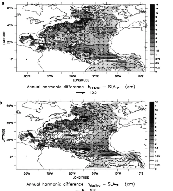
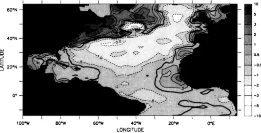
Changes in upper ocean temperature and salinity result in a steric contribution to the sea level variability which was observed first by Patullo et al. [1955]. Wang and Koblinsky's [1996] analysis of altimetric sea level data show that this contribution dominates the large-scale seasonal variability in the northeast Atlantic. This is also supported by the work of Chambers et al. [ 1997] and Stammer [ 1997]. To illustrate the seasonal signal, we present in Figure 1 the annual harmonic of the large-scale sea
Also at Mtt6o France, SCEM/PREVI/MAR, Toulouse, France
Copyright 2000 by the American Geophysical Union. Paper number 1999JC900296.
0148-0227/00/1999JC900296509.00
level anomaly from TOPEX/Poseidon (T/P) altimeter measurements for the period October i 992 to September i997 (data processing is presented in section 3.2). On Figure 1 the annual amplitude is indicated by contours and the phase (date of maximum) is given by the orientation of the vector (January 1 at
12 o'clock, increasing clockwise). North of 20øN the sea level seasonal oscillation reaches a 5 cm annual amplitude, with somewhat higher values in the Gulf Stream region. The phase is rather constant (maximum in September) over the whole extratropical part of North Atlantic. In the tropics the phase has a stronger spatial variability, and the amplitude varies from < 1 to 8
crn at 5øN, northeast of South America.
Numerical Ocean General Circulation Model (OGCM) experiments at coarse resolution have been used to study the seasonal sea level variability [Stammer et al., 1996; Fukumori et al., 1998]. These numerical models suggest that the deeper steric changes and the bottom pressure changes do not contribute much to the large-scale seasonal sea level variability at midlatitudes, with the main contribution from steric changes induced by the surface heat fluxes. In this study we present a refined test of this hypothesis for the North Atlantic. In particular, the relative magnitude of the different contributions to sea level seasonal variability is carefully evaluated, either directly from observed data or from an OGCM simulation. We have to rely on an OGCM simulation for the advection and bottom pressure seasonal changes which cannot be accurately estimated from in situ observations. These results from the simulation are applied as corrections to real sea level data to investigate if the sea level budget is closed within the observational uncertainties. This is
6308 FERRY ET AL.: SEASONAL SEA SURFACE HEIGHT IN THE NORTH ATLANTIC OCEAN 60ON - 40ON - LLJ -- J 20ON 0 ø I I 90øW 70øW 50øW 30øW 10øW 10øE LONGITUDE
Annual harmonic, SLATp (cm)
Figure
1. Annual
harmonic
phase
and
amplitude
of the
sea
level
as
measured
by
TOPEX/Poseidon
(T/P)
during
the
period
from
October
1992
to September
1997.
Amplitude
is proportional
to the
length
of the
vector
and
the
date
of
the
maximum
is given
by its direction
(January
1 at 12 o'clock,
increasing
clockwise).
Contours
represent
the
annual amplitude (in cm).12
10
done for the average seasonal cycle from 5 years of T/P altimctric data (October 1992 to September 1997) with the stcric effect evaluated from heat fluxes taken from operational meteorological models as well as from climatologics.
The OGCM wc use is at a higher resolution (1/3 ø) than some of the previous ones. It includes a mixing scheme that is based on a simplified equation for turbulent kinetic energy. The model is forced with daily European Centre for Medium-Range Weather Forecasts (ECMWF) rcanalysis fields. The period of the forcing (1989-1993) is, however, different from the one wc investigate for the sea level data. Nonetheless, wc expect that the seasonal balance in the simulation should bc representative for the T/P period as well. Wc arc also aware of the fact that the observations, in particular the heat fluxes, have errors, which wc would like to quantify from the sea level budget.
ocean), the first term on the right-hand side represents the change in heat content integrated vertically to a depth z, and the second term represents the effect of the advective terms on the hem content change of the upper water column (this includes
horizontal and vertical advection as well as horizontal and
vertical diffusion). Over most of the ocean the density p and
specific
heat
cp vary by <1%, so that assuming
that they are
constant introduces very little error. Angle brackets represent an appropriate spatial averaging to be defined below. Gill and Niiler [1973] have discussed how the relative magnitude of the advection term <ADVr> is sensitive to the scale retained; the larger the scale, the less its relative importance.The heat content can be related to the temperature-induced steric change of the upper water column [e.g. Chambers et al., 1997, Gill and Niiler, 1973] by
f (p cp
T) dz
= p cn/,4
(SSH
- h
s - hoc
- hot
),
2. Methodology
where SSH is the sea surface height, hs is the contribution of the
The
basic
balance
we will discuss
can
be summarized
in the steric
change
related
to salinity
change
assuming
a constant
following
way:
temperature,
hoc
is the
contribution
of deeper
steric
change
(from
< Q > = •t < f(P
c• T)
dz
> - < f(p c• ADVz•
dz
>,
depth
z to
bottom),
and
hbtis
the
sea
bottom
pressure.
Here
1/,4
is
a vertically averaged thermal expansion coefficient (see
FERRY ET AL.: SEASONAL SEA SURFACE HEIGHT IN THE NORTH ATLANTIC OCEAN 6309
< Q > = Ot
< p ct,
/A SSH
- p ct,
/A ( hs
+ hbc
+ hbt
) >
- < f(p cp
ADVz9
dz>,
(1)
where we will evaluate to which extent the balance between the
first two terms holds. A has a seasonal cycle, and because the average seasonal temperature variability is mostly annual in the North Atlantic [Levitus, 1984], A also varies mostly at the annual harmonic. This will induce a contribution due to nonlinear combination between 1/A and the steric height which will be mostly semiannual. We also checked that nonlinear combinations of semiannual harmonics of these components produce only negligible annual variability. We will only discuss the annual harmonic of the different terms of (1), so that at each individual location A can be taken as a constant (this was tested in the model simulation; see also the discussion in the appendix). We decided not to consider the semi-annual harmonic because of the large error on the sea level semiannual harmonic resulting from aliased tides in the TOPEX-Poseidon data set [Schlax and Chelton, 1994]. Finally, at midlatitudes the semiannual contribution to sea level observations is small and not easily extracted from the background variability.
The results from (1) can be presented in heat flux units (W
m-2).
Here
we chose
to integrate
the equation
in time and
to
present the budget in equivalent sea level units (cm), i.e., the unit of the sea level observation that is central to the study:
A/(p
ct,
) f (< Q >) dt = < SSH
> - < (h
s + hbc
+ hot
) >
-,• f (< fADVrdz >) dt.
(2)
The integration constant has been chosen such that the annual mean of each term is zero. Different spatial scales have been considered. We will present the results for spatial averages in 5 ø x 7 ø latitude by longitude boxes, after removing data on shelves shallower than 300 m. This smooths the fields retaining the main large-scale structures. At midlatitudes this averages out most of the baroclinic wave activity at seasonal to annual periods.
The annual harmonic of the different terms of the model
simulation as well as of the observations will be estimated by a least squares fit in a multiple function regression of the time series (annual and semiannual harmonics, trend). The error on the
estimated annual harmonic results from the residual to the
regression. The estimate on terms for which there is a large unexplained variance will be less certain, and their magnitude will also be less than what would be obtained from a simple Fourier decomposition. This will affect each term differently. It will probably be larger for the bottom pressure term, which in model simulations at midlatitudes, has a large high-frequency component [Fukurnori et al., 1998; Stammer et al., 1996]. With the observations we have only hints on some of the terms and some have large errors, in particular the heat fluxes. For the simulation we can quantify all terms of the budget (2). Some of them can deviate significantly from the reality because the average model circulation can be different from what is observed. The seasonal vertical motions depend on the wind forcing, which has some errors, and the simulation of diffusive processes, especially in the extratropics, certainly lacks realism.
After presenting the model simulation used and the data sets from which we estimate the heat budget, we will successively present the different terms of (2) in the model simulation, focusing on whether they are representative of the real ocean. We will then discuss the comparison of TP sea surface height and the heat fluxes for the period from October 1992 to September 1997.
3. Numerical Simulation and Data Sets
3.1. Numerical Simulation
The ocean model is derived from the high-resolution (1/3 ø x 2/5 ø latitude by longitude) version of the Community Modeling Effort (CME) primitive equation model [Bryan and Holland,
1989]. The domain is the North Atlantic between 15øS and 65øN with relaxation near the boundaries to the climatological temperature and salinity fields of Levitus [1982]. The present configuration uses a refined vertical grid with 37 levels spaced more closely near the surface. The layer thickness is 11 m near
the surface and increases to 30 m at 150 m and 250 m below 1000
m. A simplified turbulent kinetic energy equation [Blanke and Delecluse, 1993] has been included [Oschlies and Garqon, 1999] which contributes to a more realistic description of turbulent mixing than in the earlier version of the model.
The model is forced by daily wind stress x in the momentum equation and by the surface turbulent kinetic energy input u *• in
the turbulent
kinetic
equation
for the surface
layer
(u* = (•/p)•/2).
The heat flux at the surface consists of a prescribed flux Qo taken from the daily ECMWF reanalysis plus a relaxation term R T
(Ts
øbs
-Ts),
where
T
s is the model
sea
surface
temperature
(SST)
and Ts
øbs
is the weekly
SST field [Reynolds
and Smith,
1995]
used by ECMWF for their reanalysis. The relaxation constant RT is computed following Barnier et al. [ 1995]. It has a geographical dependency similar to the climatology of Barnier et al. [ 1995] but was chosen to be constant in time (R T ranges from 20 to 45
W m -2 K-•). The freshwater
flux at the surface
consists
simply
in
a relaxation toward the monthly sea surface salinity climatology from Levitus and Boyer [ 1994] with a relaxation constant chosen as 1/15 days. For heat and freshwater flux at the surface the relaxation terms guarantee that the simulation is not very far from the observations, at least for the mean state (see Barnier et al. [1995] for a detailed discussion). They can, however, induce lags in the simulated SST and sea surface salinity with respect to the observed variables. They can also affect vertical stratification and therefore mixing and water mass formation, in particular in the Gulf Stream and North Atlantic current areas [New et al., 1995]. The fluxes are applied in the first layer, except for penetrative solar radiation for which clear open ocean water is assumed.
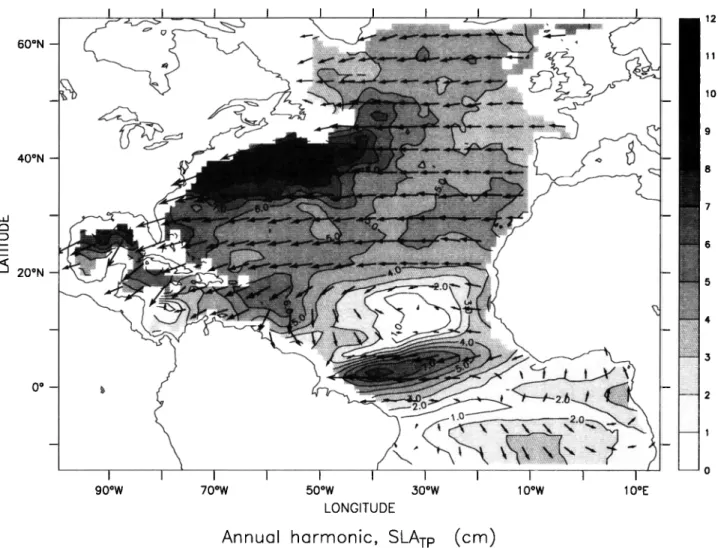
The initial state is taken from a 37 year long simulation of the average seasonal cycle. This long simulation is described by Oschlies and Willebrand [1996] and used Hellerman and Rosenstein [ 1983] wind stress climatology and surface heat flux parameterization of Han [1983]. The model is then forced by daily fields from the ECMWF reanalysis for the period 1989- 1993, and the years 1991-1993 are considered in the analysis. The average model circulation for this period presents many realistic current features (Figure 2). However, its Gulf Stream separates
from the American continent too far north and a North Atlantic
Current (NAC) with a very intense branch flows toward Iceland in the central subarctic gyre. The simulation lacks a well-defined Azores Current in the eastern Atlantic. These defaults are, however, typical of present eddy-permitting models (see the model intercomparison by Dynamics of North Atlantic Models (DYNAMO) Group[1997]). The tropical seasonal circulation is reasonable, which is also typical of other simulations with a similar resolution [Blanke and Delecluse, 1993; B6ning and Herrmann, 1994]. This simulation has a too intense convection in the Labrador basin, a reasonable meridional overturning, and a distribution of late winter mixed layer depths which is relatively realistic, in particular the relatively deep trough extending across
6310 FERRY ET AL.: SEASONAL SEA SURFACE HEIGHT IN THE NORTH ATLANTIC OCEAN 60øN 40øN '• 20ON
oo-
!
! ooow I I80ow 60ow 40ow 20ow OOE
LONGITUDE
meon velocity ot 50m depth (cm/s)
> 50.0
Figure 2. Annual harmonic phase and amplitude of the sea level as measured by TOPEX/Poseidon (T/P) during the period from October 1992 to September 1997. Amplitude is proportional to the length of the vector and the date of the maximum is given by its direction (January 1 at 12 o'clock, increasing clockwise). Contours represent the annual amplitude (in cm).
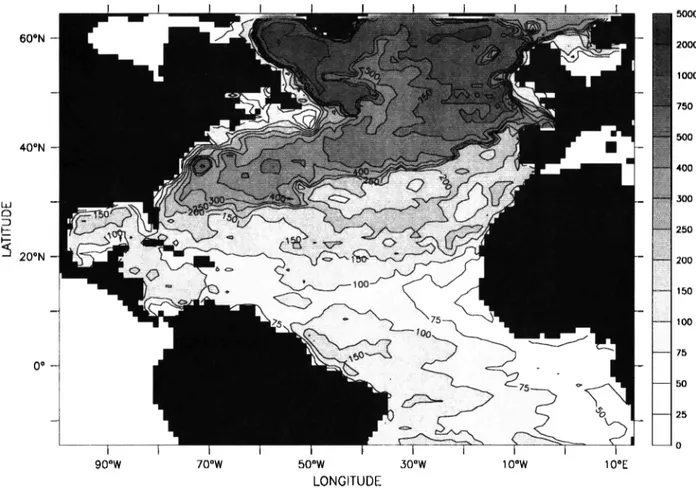
the entire basin along the northern edge of the tropical gyre and the shoaling toward the equator in the subtropical gyre. Figure 3 presents the maximum mixed layer depth Hma x attained at each grid point during the 5 year simulation (using a Ap - 0.125 kg m '3 criterion), which is much larger than a temporal average of winter mixed layer depths. This often explains why Hma• is larger than in climatological fields, for example, Lamb [1984]. There is, however, a tendency to have larger than observed mixed layer depths south of the NAC (which is farther north and west than observed) and also in the eastern North Atlantic, north of 45øN and east of 30øW. This is related to the simulated path of the NAC, which does not penetrate far enough eastward [e.g., Oschlies and Willebrand, 1996]. Nevertheless, we decided to use Hma x as the lower boundary for the vertical integration of the model heat equation (equation (2)).
The average deviation of modeled SST from the observed SST is presented for the average winter and summer (Figure 4). It indicates that the differences are larger in winter (except near the equator), an expected result because during the summer, with shallow mixed layers, the relaxation term will be more effective in bringing the SST close to observations. The winter pattern in particular clearly indicates the path of the Gulf Stream being too far to the north, and the resulting strong advection of warm water toward the Irminger and Labrador Seas. Rather large SST deviations are found in the upwelling areas, where the relaxation term has little effect on the sea surface temperature. There is a seasonal cycle in the temperature corrective term, which is much less than the amplitude of the ECMWF heat fluxes.
3.2. Altimetric Data
We use a 10 day gridded (0.25 ø x 0.25 ø) data set produced by objective mapping of the corrected T/P altimetric sea level data [Le Traon et al., 1997]. The first guess is a spatial average of all the data within a 5 ø radius. The usual corrections are applied, in particular the electromagnetic bias correction from Gaspar et al. [1994]. An improved correction for the inverse barometer effect (P-Pref) was applied using ECMWF atmospheric sea level pressure P [Dorandeu and Le Traon, 1999]. Instead of assuming a constant reference pressure Prefequal to 1013.3 mbar, Pref was calculated as the average sea level pressure over the world oceans, including the Arctic. The principal tidal constituents from the model CSR 3.0 [Eanes and Bettadpur, 1995] are removed (long period tides are not removed). Data on the shelves are removed before spatial filtering. The average seasonal variability is estimated for the period October 1992 to September 1997 (5 years). This estimate is representative of the 5 years selected with an uncertainty which results from the error on the data and from the variability at other frequencies. For the spatially averaged data we consider, this results in an rms uncertainty in the annual harmonic amplitude and phase of 6% and 4 ø in the eastern Atlantic to 6% and 3ø in the Gulf Stream area (see section 5 for a description of this uncertainty estimation). There is also the possibility that this product has seasonally dependent biases. On the basis of comparisons with tide gauge sites in the North Atlantic (in particular at Ponta Delgada, Azores) we estimate that the monthly fields are accurate to within 1.6 cm rms difference,
FERRY ET AL.: SEASONAL SEA SURFACE HEIGHT IN THE NORTH ATLANTIC OCEAN 6311 60øN 40øN LLI
<• 20ON
0 o I I I I I 90øW 70øW 50øW 30øW 10øW 10øE LONCITUDEFigure 3. Maximum mixed layer depth Hma x (m) during a 5 year integration of the model. A Ap=0.125 kg m -3 criterion is used to determine the mixed layer depth.
5OOO 2000 lOOO 75O 5OO 40O 300 25O 2OO 150 100 75 50 25
including systematic seasonal biases. Annual amplitude and phase of Ponta Delgada tide gauge and T/P measurements at that location were found to be in agreement to within 1 mm (---2% of the annual amplitude) and 4 ø , respectively.
3.3. Other In Situ Data
Because of uncertainties on the model circulation we will also
use a data set of near-surface currents to independently estimate
the effect of horizontal advection. Horizontal advection of heat is
estimated from upper ocean currents and monthly SST maps [Reynolds and Smith, 1995] by assuming a 150 m deep mixed layer and letting the currents advect the SST field. This very simple calculation does not properly take into account the advection below the seasonally varying mixed layer, which is difficult to estimate from very scarce in situ temperature profiles and velocity fields. The average currents are constructed from drifter velocities provided by NOAA/Atlantic Oceanographic and Meteorological Laboratory (AOML) and the Ice Patrol. The drifters are all drogued World Ocean Circulation Experiment (WOCE) drifters and should be current followers to within I cm
s
-] for typical
wind
conditions
in the
North
Atlantic
[Niiler
et al.,
1995]. Most of the drifters are drogued at 15 m (the Ice Patrol drifters were, however, often drogued at 50 m). Different regions have been sampled at different times, but a large part of the data corresponds to the period 1993-1998 and is therefore nearly simultaneous with the altimetric data set. Most major currents north of 25øN have been sampled during that period, with the
exception of the Gulf Stream south of Cape Hatteras. The Gulf Stream, after its separation off Cape Hatteras, and the NAC are well sampled, but because of the large eddy variability in this area the average currents still have large uncertainties. One should also mention that a large part of the drifters in the Gulf Stream have entered the current from the north (major deployments were in the Mid-Atlantic Bight and in the vicinity of George Bank).
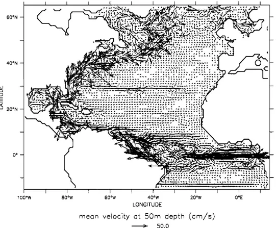
The data have been gridded on a 0.5 ø x 2 ø latitude by longitude grid, which captures a large part of the structure in the average currents and their quasi-stationary meanders or eddies (for instance, in the NAC, east of the Grand Banks). These boxes are large enough so that most of them north of 25øN have at least 15 days of drifter data, which we find to be an absolute minimum to approach the average circulation in the presence of the energetic eddy field. An illustration of the resulting circulation in the eastern Atlantic is presented in Figure 5, which shows few
currents
>5 cm s
-]. The NAC is well represented
with strong
eastward current branches at 34.5 ø (the Azores Current), 45 ø, and 52øN. We also decided to substract an averaged Ekman component of the current at 15 m using a method described by van Meurs and Niiler [1997]. The wind stress used for this computation is taken from the ERS weekly wind stress product.To reconstruct the current field at any given time, we add to this average current the geostrophic current deviations based on smoothed altimetric sea level fields and an Ekman velocity distributed over the 150 m layer which is estimated from the ERS weekly wind stress product. In order to justify the calculation of
6312 FERRY ET AL.: SEASONAL SEA SURFACE HEIGHT IN THE NORTH ATLANTIC OCEAN 60øN 40øN I•J .,• 20ON 1 O0øW 80øW 60øW 40øW 20øW OøE LONGITUDE
SST model-Reynolds, for winter (J-F-M)
deg. C
lO 5 2 1 0.5 -0.5 -1 -2 ß -3 -5 -10 60øN 40øN .• 20øN 100øW
:--:-:-
-::::•':-';::!::i!i:i!'i:i'iit:'½:i:½;i!?a-'½..i•'•':
"••:...•...
'••i• :-""-•j*,
•'"'
'""•:'""'
.il,_:i',•/?,77!':-'.';::
': .,--:•i;iiaX
':::;c
;?:
.*... ;" ::i::-.'•:!?• ""-" - --. --=c' r'-.-.., ,-' •: --::'----:-%?':-*!:-•:i:_.ii;;_•i!::i'_--;_;::ii,_?.--::•; .:::,-...-'--' ... ß ,;._. ':'i'i: _-
... ...
.:.:..,__,,:,,,.,.
;';'.Zi?,;;,7::'
¾'
...
.';-*-'-!-'?-:-'3::i:.%
---'"-•:
...
-,•-?i?.+g.':
...
'-'--,
...
--•:.::::,:':•½?.'.%:;;•,;i?;;.'
-%,*-:.-'-. •::'; T--"_,.*...,.:** r...-.•:?:*::?% ... i:..(:-.!..-'i,!:U:'.:L..!:;i:•-..'i..'.:_-.. ;-,'- .•;-;--":' ...'-
80øW 60øW 40øW 20øW OOE
LONGITUDE
SST model-Reynolds, for summer (J-A-S) deg. C
lO 5 2 -0.5 -2 , -5 -•0
Figure 4. Deviation of the modeled SST from the observed SST for the last 3 years of simulation averaged over (a) winter (January-March) and (b) summer (June-September) months (in øC).
advection described above, we have performed a comparison between the horizontal advection diagnosed in the model and a composite advection product calculated in the same manner described in this section and using model outputs. The results show that the composite advection field overestimates the amplitude of the advection field over the whole basin. It is, however, interesting to consider this advection estimate from data because it is completely independent from the model simulation. It should be an upper boundary for the real horizontal advection annual amplitude in the upper layers of the ocean.
We have also used temperature profiles from expandable bathythermographs (XBT) data in an area which has been regularly sampled since 1992 in the eastern North Atlantic (between 40 ø and 25øN and west of 40øW) to estimate directly the seasonal changes in steric height above 700 m, separating the contributions of the near-surface layer above the winter thermocline and of the deeper layer.
4. Sea Level Budget
4.1. Annual Heat Fluxes and Sea Level From the Model
Simulation
The simulated SSH annual harmonic (Figure 6b) presents its largest variability near the model Gulf Stream (>9 cm) with a maximum near day 270. In the subtropical gyre, there is a large band with an amplitude between 4 and 5 cm (and an earlier phase of the maximum near day 240) with amplitudes decreasing toward the northeast and south of 20øN. Closer to the equator, there is more structure in the field with two bands of larger variability centered near 10øN and near the equator in the western Atlantic and an area of large variability in the Gulf of Guinea.
The steric variability induced by the simulated heat flux (Figure 6a) also presents a maximum amplitude in the Gulf Stream with an amplitude decreasing regularly toward the south
FERRY ET AL.: SEASONAL SEA SURFACE HEIGHT 1N THE NORTH ATLANTIC OCEAN 6313
•
..,
_t•--,"
,,"' , ..,."• _ / ...--
_./ _.///
II / •• • n • • • a /L• --x
/
x I /
/
'
•
x -
x
•
I
1-,
x
x ' '
,
Y . lq
1
r ' ' ' ' ' ' - - - ' ' ' / k' ' 20øN • I I ! 40ow 30øW 20øW 10øW LONGITUDEmeon 15m velocity from drifters (cm/s)
20.0
Figure 5. Mean currents at 15 m depth gridded on a 2 ø x 0.5 ø longitude by latitude grid from drifter velocities in 1993-1998 in the eastern North Atlantic (cm s']).
and presenting a minimum near the equator. North of 20øN, the amplitude is often less than the one in the sea level (except in the eastern North Atlantic), but the phase agrees very well with that
of the sea level. The difference between the annual harmonic of
sea level and the one in the steric variability induced by the heat fluxes is presented normalized by the amplitude of the sea level annual harmonic on Figure 6c and can be considered an estimate of the unexplained variance. Within 15ø-20 ø of the equator this ratio is large, and a large part of the signal in sea level cannot be explained by the heat fluxes. Farther north, there is a large area in the range 0.1-0.2, increasing north of the Gulf Stream in the northwest Atlantic to >0.3. In the simulation, where the budget is perfectly balanced, this has to be explained by the other terms of (2).
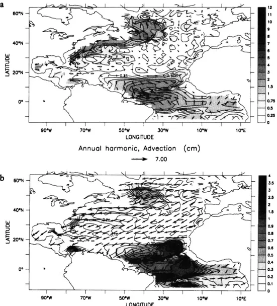
4.2. Advection Term
First, we consider the advection term of (2) integrated from the surface down to Hrnax (Figure 7a) in the model simulation. This term has an amplitude of <0.5 cm in a large part of the
domain
(equivalent
to <20 W m
'2) where
it represents
<20%
of
the sea level signal (Figure 7b). The rms uncertainty on the amplitude is <0.25 cm in large parts of the eastern Atlantic and subtropics. The advection term is larger in the Gulf Stream, where the maximum is reached near day 220-270, which suggests that it contributes to a larger sea level variability than one would expect from the heat flux alone. It increases near the equator and
in the Gulf Stream. The contribution due to advection is weakest
in the eastern North Atlantic, where its does not exceed 0.25-0.5
cm. In the tropics the advection term presents a structure similar to the one in sea level but with smaller amplitudes. There it originates mostly from the vertical advection associated with the seasonal displacement of the thermocline, resulting from the seasonal wind forcing [Merle and Arnault, 1985]. In that sense, it should be considered together with the deeper steric contribution hoc (Figure 8a), which has a similar structure (see below).
The only term we can estimate from data is horizontal
advection
(the dominant
contribution
in the model
simulation
north of 20øN). This is done for the 5 years from October 1993 to September 1997 as described in section 3.3. The annual harmonic of the estimated advection is computed and smoothed on the same grid as the model results, and we separate the component associated with the geostrophic currents (Figure 7c) from the part associated with the variable Ekman component (Figure 7d). The contribution of the Ekman currents is usually less than the one of the geostrophic currents, and they often have the same phase. Not surprisingly, the two terms have large values in the Gulf Stream and smaller values in the eastern Atlantic. In the western Atlantic, this estimated horizontal advection has amplitude and phasesomewhat
similar
to (A f < f A DV r dz > dO in the model
simulation, but it is much less important north of 50øN (clearly, this suggests a deficiency of the simulation in the subarctic gyre). In the data, there is a suggestion of a tongue of larger (0.5-1 cm) variability near 40ø-45øN toward the eastern Atlantic, which is not found in the simulation (and with a different phase). There is also a band of large values (1 cm) near 20øN west of 40øW, which is not found in the model simulation and which is certainly
6314 FERRY ET AL.: SEASONAL SEA SURFACE HEIGHT IN THE NORTH ATLANTIC OCEAN -- 7 • • 2 O" • .:1•..• ... I I I I 1 o go'w 70'W 50'W 50'W 10'W 1 LONGITUDE
Annual
harmonic
hQnet
model (cm)
•-- 7.00b 60ON
--
40eN• 20"N
0 o 90øW 70øW 50øW 30øW 10øW 10øE LONGITUDEAnnual harmonic $$H model (cm)
• 7.00 12 -- ;• •5 2 1.5 1 0.5 0.25 0 c 60ON -- 40ON -- u • --
g 20ON
• 2.5 2 1.5 0.8 0.7 :=-. 4 ... ::=':'.';•S:d '.L.•.: -':::; -• •- ' .: ':' •''•- , ' ...
;:
'-."
-'•,• •
• ....
A.•
!':•?'•
0.5
'-h•
-•,
.. :,-•,' .-:.-...•¾._-•--.•.•.•
:S•...._._.-..•-•2.;.
•.
....
. :•
0.3
o.,
o 90øW 70øW 50øW 30øW 10øW 10øE LONGITUDE >- 5.00FERRY ET AL.' SEASONAL SEA SURFACE HEIGHT IN THE NORTH ATLANTIC OCEAN 6315 60ON -- 40ON -- i--
• 20ON-
0 o - _•_ ... • • .•
...
• •?'
•__;::-;-:._:¾'i::_;?:_•
•
0.5 0.25 I I I I I I I I I I o 90'w 70-w 50-w 30-w 1 o'w 10'E LONGITUDEAnnual harmonic, Advection (cm)
7.00
b 60ON
40øN• 20ON
90oW I I I I I70øw 50øw 30ow 1 oow 100E
LONGITUDE 4 5.5 5 2.5 2 1.5 0.9 0.7' 0.6 0.4 0.2 0.1 0
Figure 7. (a) Same as Figure 6a but for the simulated advection (in cm). (b) Annual harmonic of the simulated advection normalized by the annual harmonic amplitude of the simulated SSH. The length of the vectors is proportional to the nonnormalized difference (in crn). (c) Same as Figure 7a but for in situ estimate of geostrophic advection estimated from data. (d) Same as Figure 7a but for in situ estimate of Ekman advection estimated from
data.
due to an undersampling of mean velocity by drifting buoys in this area and to an incorrect description of the vertical structure of the temperature gradients. The uncertainty on this estimate from data is difficult to ascertain, as it originates also from systematic errors in the average current field and in the estimate of the vertical structure of currents and horizontal temperature gradients.
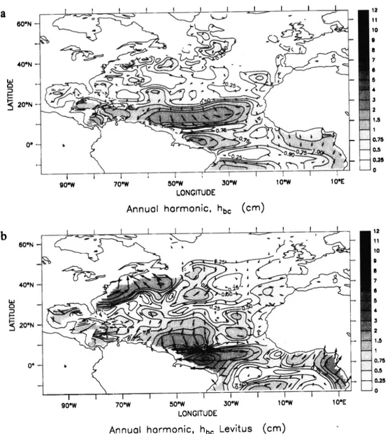
4.3. Deeper Steric Contribution
In the tropics the deeper steric contribution h bc in the model simulation (Figure 8a) has a structure similar to the one of the
advection term. This is expected because the advection term in the tropics results, to a large extent, from vertical advection of the thermocline, which also contributes greatly to ht, c. Notice that the maximum amplitude near 10øN extends farther west than for the advection term and that it has a smaller amplitude in the western equatorial Ariantic. The deeper steric contribution is small almost everywhere north of 20øN (0.25 crn or less), where it is rarely significant (based on the rms uncertainty) and where it is always
smaller than the advection term.
Here hbc can be compared with estimates from climatological monthly temperature and salinity fields [Levitus and Boyer, 1994]
Figure 6. (a) Annual harmonic phase and amplitude of the heat flux induced steric height of the model. Note that this component includes the relaxation term of the surface heat flux parameterization. Amplitude is proportional to the length of the vector and the date of maximum steric height is given by its direction (January 1 at 12 o'clock, increasing clockwise). Contours represent the annual amplitude (in cm). (b) Same as Figure 6a but for the simulated sea surface height (SSH). (c) Difference between the model SSH and heat flux induced steric height annual harmonics normalized by the amplitude of SSH. The length of the vectors is proportional to the nonnormalized difference (in cm).
6316 FERRY ET AL.: SEASONAL SEA StIRFACE HEIGHT IN THE NORTH ATLANTIC OCEAN 60ON - 40øN • 20øN 0 o 1 0.75 0.5 0.25 I I I I I I I I I o 900w 700w 500w 30'w 1 oow 1 LONGITUOE
Annual harmonic, 9eosirophic advection (cm)
8
6
21.5
0.5 0.25 o7oow 5oow 3oow
LONGITUDE
Annual harmonic, Ekman advection
(am)
Figure 7. (continued)between
Hma
x and 1000 m. Notice that the climatological
temperature fields are rather well constrained, at least above 800 m, but that the salinity fields are based on a rather coarse sampling which does not constrain well the monthly fields, resulting in larger errors. The calculation of Hma x is done using the same mixed layer criterion as for the model but is based on the average monthly fields. Mesoscale processes, interannual variability in the surface forcing, and baroclinic wave propagation all contribute to a deeper Hmax in the model than in the Levims and Boyer [1994] climatology. However, we believe that similar physical processes are present in the simulation and in the climatology at the annual period, independent from the depth of the mixed layer.
This climatological estimate (Figure 8b) presents a large spatial variability at midlatitudes. Its annual harmonic has an amplitude >1 cm south of 30øN, as well as near 35øN west of Gibraltar and between 35 ø and 50øW (the phase is quite different between the two areas). These results are coherent with previous studies (for example, at 33øN, 22øW, Strarnrna and Siedler [ 1988] document a warming in the early months of the year at 200 m). There is also a large variability north of the Gulf Stream
which is not found for the equivalent model term, as for most of the variability north of 20øN. South of 20øN, there is more similarity between the two fields, although the large amplitudes near 10øN in the data are confined farther west than in the simulation, and the western equatorial maximum is more present in the climatology. The latter is coherent with other analyses of the equatorial Atlantic seasonal cycle [Merle, 1980; Merle and ,4rnault, 1985].
To complement this analysis of the climatology, it is possible to estimate the seasonal steric variability integrated to 700 m on the basis of individual temperature profiles (XBT). We chose profiles from the years corresponding to the altimeter data (October 1992 to September 1997), but we could similarly have considered data collected for the years of the simulation (1989-
1993) with little difference. In the northeast Atlantic, the data coverage is mainly adequate between 40 ø and 20øN, east of 45øW. Except in the northwest comer of this domain, the winter mixed layer depth is usually <150 m, which we select as the lower boundary of the upper layer. The annual steric contribution of the layer above 150 m is relatively uniform, with smaller values in the eastern part of the domain as well as south of 25øN
FERRY ET AL.: SEASONAL SEA SURFACE HEIGHT IN THE NORTH ATLANTIC OCEAN 6317
40ON
_
1C•
-
I
I
I
I
I
I
I
I
•0
90oW 70oW 50oW 30oW 10=W 10=E
LONGITUDE
Annuol hormonic, hbc (cm)
4• 10 :•:•:., 1.5'•::•
0.75
0 • _ 0.25 •0gOoW 70oW 50oW 50øW 10=W 10=E
LONGITUDE
Annuol
hormonic,
hbc Levitus (cm)
Figure
8. (a) Same
as
Figure
6a but
for the
simulated
deep
steric
component
hbc.
(b) Same
as
Figure
8a but
for the
monthly
œevitus
and
Boyer
[ 1994]
climatology.
Steric
height
is integrated
betweenHmax
(obtained
from
œevitus
and
Boyer
[1994]
atlas)
and 1000
m. (c) Upper
ocean
(0-150
m) steric
height
annual
harmonic
from expandable
bathythermographs
(XBT) profiles
collected
during
1992-1997
(in cm).
Profiles
are
binned
in 5 ø x 4 ø longitude
by
latitude boxes. (d) Subsurface (150-700 m) steric height annual harmonic from (XBT) profiles.(Figure 7c). This is very similar to what is found with the climatology. Other details of the distribution are within the uncertainty caused by the sampling and the eddy variability. The contribution to steric sea level below 150 m is much less, with
larger
uncertainties,
in particular
in the central
part
of the domain,
which is not as well sampled (Figure 7d). There is, however, some indication for a seasonal cycle in the northeastern part of the domain (north of 36øN) with maximum values in March (<1 cm). This is larger than what is found in the simulation and could result from the seasonal Ekman pumping. This component is smaller in the model simulation probably because the depth of integration for the upper layer is particularly large (---300 m; see
Figure
3) and thus
includes
a large
part of the Ekman
pumping
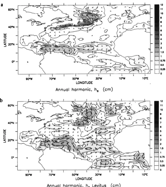
component near the thermocline. 4.4. Surface Salinity
In the model simulation the contribution of salinity variations in the mixed layer, hs, is also smaller than the advective term but
is well defined with only small rms uncertainties. It can reach 1 cm near and north of the model Gulf Stream (Figure 9a). It is also rather large near 15øN and, in particular, north of Venezuela. The
salinity
changes
in the upper
layer
result
from
a combination
of
advection-diffusion and surface forcing (relaxation toward
monthly
climatology).
In contrast
to the temperature
equation,
the
relaxation term for salinity is large in many areas compared with the observed freshwater forcing (ECMWF reanalysis). Forexample,
the annual
amplitude
of the simulated
freshwater
flux in
the Gulf Stream
reaches
200 cm year
-1, compared
with a
freshwater
annual
component
of 60 cm year
'1 in the ECMWF
reanalysis (the Gulf Stream path being too far north displaces the salinity gradient north of its normal position). This directly
affects
the
seasonal
cycle
of surface
salinity,
wi,th
t•h•
relaxation
term introducing a spurious phase difference with respect to the climatology.Therefore we also estimated what would have been the seasonal cycle of hs assuming that the model salinity was the
6318 FERRY ET AL.: SEASONAL SEA SURFACE HEIGHT IN THE NORTH ATLANTIC OCEAN
C 46øN
15
14 15 42ON 12 11 lO 38ON 9 8 • 34ON 6 4 30ON 3 2 1 26•N 0.75 0.5 0.25 22øN I I I I I 0 45ow 35øW 25øW 15øW 5øW LONGITUDEAnnu(}l
h(}rrnonic,
upper oce(}n (0-150m)steric height
> 5.00
46ON J I I I I I I I I
42
o
N : -- A•"-"
---'-'---:
"-•½•::-:•i•i•::..•:•i•:-
-.
:-::
:-:' - -:-•:--:.
':::,:.:':
:.::::
:':'>..::-•;
:.::--:i•
:::..:-::
:"-:-::
:-:
•--::--:.:.:
:':':.-'-::.:•
.:.:
:.:-:':
'-
38øN
••g-L'_.??:!•
"•
-•-::•.•-..•-'
_:-.
...
:':":"•
:-:-:-.T-"'"'4'••••::•.11:•i-i'i:•.:i•i
i_•!
iii':ii-:i:!:!-i.:
'!- '"'
ß
26øN
i:
' '"!:'"'
• •
22ON
45øW 35øW 25øW 15øW 5øW
LONGITUDE
Annuol h(}rmonic, subsurfoce (150-700m) steric height (cm)
> 5.00 15 14 13 12 11 10 9 8 7 6 5 4 3 2 1 0.75 0.5 0.25 0 Figure 8. (continued)
climatological salinity [Levitus and Boyer, 1994] (Figure 9b). The results are quite different from the ones in the simulation. There are large values in the subpolar gyre (corresponding to a sea level maximum in the autumn, an effect nearly opposite to the one in the model), weak values south of 40øN and in the eastern North Atlantic, and larger values south of 20øN. There the estimate from climatology is somewhat larger than in the simulation, but its amplitude remains <1 cm, except in the vicinity of South America. The position of the band of high values associated with the Intertropical Convergence Zone (ITCZ) is centered farther south in the climatology (close to 10øN) than in the model (close to 15øN). The climatology also suggests very small values in the eastern Atlantic but presents more spatial structure. This spatial structure might, to some extent, originate from errors, the seasonal salinity fields being not too well resolved. Estimates from the climatology in the tropics are somewhat smaller than in the simulation. This suggests that the climatology has not resolved well the large seasonal tropical variability (Dessier and Donguy [ 1993] provide a better sampled surface salinity seasonal climatology which has a larger seasonal amplitude than the climatology we used).
Away from major currents or upwelling areas one expects that the upper ocean salinity seasonal signal can be estimated from the net freshwater seasonal cycle. Assuming that this is the only term in the salinity equation (i.e., neglecting advection), an estimated salt content of the upper ocean can be computed, from which h s can be derived (Yivier et al. [1999] provide details about this calculation). This was done both with the ECMWF evaporation minus precipitaion (E-P) fields for the simulation y•rs and with the Comprehensive Ocean-Atmosphere Data Set (COADS) E-P fields constructed by da Silva et al. [1994]. The two fields are more similar to each other than to the simulation estimate (not shown), in particular in the Gulf Stream area. There is also a maximum near 40øN in the central Atlantic, but this does not seem to correspond to the seasonal cycle based on the salinity fields. Nevertheless, these different estimates all suggest that the annual amplitude of the salinity term is <0.5 cm in large parts of
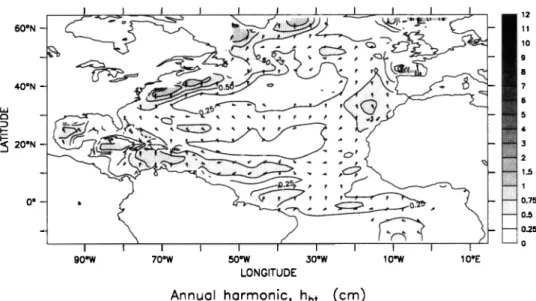
the Atlantic north of 20øN. 4.5. Bottom Pressure
In the model simulation the bottom pressure hbt generally presents a very weak amplitude (Figure 10) with very few regions
FERRY
ET AL.: SEASONAL
SEA
SURFACE
HEIGHT
IN THE NORTH
ATLANTIC
OCEAN
60ON -- 40ON --_• 20
TM
-
0 o - 60ON - 40ON - w tm -ON-
0 o m I,.•...
,:.
•c-.:•?
.:
::
•
8
_....,_,•-•
• , , :.,o:•-:-.,
- • 5
0.25 I I 090oW 70oW õOøW 30øW 10øW 10øE
LONGITUDE ---i: & ß ß • -- 9
=
_
-
0.5 -- I I I I ' I I I I 70oW 50øW 30øW 10øW 10øE LONGITUDEAnnual harmonic, h s (cm)
..-.•' ••• •' • / I I I I I I IAnnual harmonic, h s Levitus (cm)
Figure
9. (a) Sarne
as
Figure
6a
but
for
the
simulated
halinc
contribution
hs.
(b) Same
as
Figure
9a
but
for
the
monthly Levitus and Boyer [1994] climatology.6319
where it exceeds 0.5 cm. In the western equatorial Atlantic the
signal
is mostly
of baroclinic
origin
and
it contributes
much
less
to sea
level
seasonal
cycle
than
the
upper
ocean
steric
variability.
Elsewhere it is mostly barotropic, with an area of largeramplitudes
west
of Gibraltar
(closed
in this
simulation),
where
the
uncertainty
is rather
small.
In the
western
Atlantic,
part
of the
energy
results
from
the
large
background
of eddy
energy
in this
simulation,
in particular
near
the
Gulf Stream
and
north
of 45øN.
However,
before
smoothing,
there
was
an area
of amplitudes
>1
cm in bottom
pressure
with a spatially
coherent
phase
trapped
under the Gulf Stream. There is also an area of amplitude >1 cm
in the Irminger
Sea
and
south
of Greenland,
which
extends
into
the Labrador Sea•Other models have been run with somewhat different results
for this
term.
A 1
ø x 1
ø global
OGCM
has
been
forced
with
twice
daily
fluxes
(D. Stammer,
manuscript
in preparation,
1999)
which
exhibits
a low variability
in h bt in the eastern
North
Ariantic
but
with
no significant
annual
harmonic.
In that
model
the annual
amplitude
of bottom
pressure
is also
•l cm in the entire
North
Ariantic. Simulations of the wind-forced barotropic model in the
Ariantie
have
been
performed
by several
authors
[Greatbatch
and
Goulding,
1989;
Ponte,
1999].
Greatbatch
and Goulding
[ 1989]
found
a good
agreement
for the annual
phase
between
data
and
model simulation near the shelves. In these different simulations
the seasonal
amplitude
of the bottom
pressure
is of the order
of 1
cm near the western boundary current and is <0.5 cm in the eastern North Atlantic. We obtain a phase which is nearlyopposite
to Ponte's
[1999] results
for the deep
ocean.
This
suggests
that comparison
with observed
bottom pressure
variability
should
be valuable.
Unfortunately,
the only long
bottom
pressure
records
are in the equatorial
Atlantic.
These
confirm that the annual bottom pressure is small (an amplitude smaller than 1 cm [Cartwright et al., 1987]). There is an indication in the Labrador Sea based on a comparison between the annual cycle of sea level and steric change from autonomouslagragian
circulation
explorer
(ALACE)
floats
that
there
is a large
bottom
pressure
signal
(D. Roeromich,
personal
communication,
1998).
Between
Iceland
and Newfoundland,
over water
deeper
than 1500 m, a comparison of the observed seasonal cycle of steric change in the upper 750 m and of sea level suggests a smaller bottom or deep pressure signal (the summer-winter differences in sea level and steric height are 6.8 and 5.2 cm6320 FERRY ET AL.' SEASONAL SEA SURFACE HEIGHT IN THE NORTH ATLANTIC OCEAN
_• _ _
0.5
I i
I i I i o
90oW 70oW 50øW 30oW 10øW 10øE
LONGITUDE
Annual h•rmonic, hbt (cm)
Fibre 10. S•c • Fi•c 6a but for •c simu]at• bosom pr•s•c component hbt.
respectively, [Reverdin et al., 1999]). The comparison between sea level and the XBT-derived dynamic height in the eastern North Atlantic (south of 40øN) certainly also suggests fairly small
bottom pressure and deep steric signals. Although the annual o0ttom pressure signal remains therefore rather uncertain, it seems to be of a small magnitude except possibly in the
northwestern Atlantic.
5. Discussion:
Comparison
Between Observed
Sea
Level and Steric Height From Heat Flux Estimates
The simulation
confirms
that
away
from
the tropics
and
the
Gulf Stream the annual cycle of the SSH is balanced primarily byindependent observational estimates. The largest of these terms was found to be the advection term, with smaller contributions from the deep steric changes, surface salinity variability, and bottom pressure.
The model simulation shows that north of 20øN, the seasonal sea level cycle is mainly balanced by the upper ocean steric change. In the following, we additionally address the question of
whether such a balance holds when we consider the observed
SSH from T/P and the heat flux taken from an operational meteorological model. Since we have seen that the different components of (2) can be simulated by our model, we shall also
use these estimates to substract them from the T/P sea surface
height seasonal cycle in order to compare it with the seasonal the heating-induced upper ocean steric change. We have 'heat flux. First, we present in Figure I I the normalized difference discussed the other terms and have found that their respective between the annual harmonic amplitude of the heat flux induced model estimates could be compared to some good results with steric change estimated from the monthly ECMWF analysis and
60ON - 40ON -- t'• --
<• 20øN
90øW 70øW 50øW 30øW 10øW 10øE LONGITUDE lO.O 0 o ß -- 3.5 -- 2.5 ß 2 -- 0.9 0.8 0.7 0.6 0.5 0.4 0.3 0.2 0.1 0Figure 11. Difference between the T/P sea surface height and the ECMWF heat flux induced steric height annual harmonics normalized by the annual amplitude of SSH (both harmonics are relative to the October 1992 to September 1997 period). Contour lines correspond to the normalized annual amplitude harmonic of the difference. The length of the vectors is proportional to the nonnormalized difference (in cm).
FERRY ET AL.: SEASONAL SEA SURFACE HEIGHT IN THE NORTH ATLANTIC OCEAN 6321
-
• ... . • ...
:•:..,,.•..-,..
••
'
- • " ... ... ..½•:;•::•. •:•:_&..• - 40ON -- . 7• 20ON-
. . 3
0 = • 0.750.5
-- -- 0.25 •0 / /, •1 • I • I •1 4 I •1 • I I60"N
• ======================5•:;
"•
...
"'•'••-
-••:••
11
40øN 7 • ... • .__:_•i • • .... •=•=• ' . 6• 20-,
.:•
½•-
• 1.50. I _
I
0.5 0.25 I I •0 90"W 70"W 50"W 30"W 10"W 1 LONGITUDEAnnual h•rmonic difference hd•si•v
• - S•mp (cm)
• 10.0
Figure 12. (a) ß "Reference" estimate, • difference be•• • "co•ect•" T• SSH •d • ECM• heat flux induc• stsc height •ual h•onics for the October 1992 to S•t•ber 1997 •od. Conto= lines co•es•nd to • ••1 h•onic •plimde of • •fference (in cm). • T• sea level is co•t• for •e eff•t of ADV• h•, •d hs. (b) S•e • Fibre 12a but • heat flux us• is the da Silva et al. •994] climatolo•. (c) S•e • Fibre
12a but • hy•olo•cal co•tion is appli• to • T• SSH. (d) S•e • Fibre 12a but • hy•ologic• co•tion is appli• to • T• SSH •d • heat flux • is • da Silva et al. [1994] climatolo•.
of the sea level from altimctry (without any correction for advection, bottom pressure, and salt storage). Both are estimated for the period from October 1992 to September 1997. The annual amplitude and phase of this residual are rather similar to the ones in the simulation (Figure 6c), at least in the Gulf Stream and
northwestern Atlantic and south of 20øN. The differences are
somewhat larger in the eastern North Atlantic, where they reach 30% of the annual amplitude of sea level (and have a different phase than in the simulation).
We need to evaluate whether these differences can be
explained by the other terms in the equation or whether they
result from errors in the heat fluxes or in sea level. For that we will use different combinations of sea level and of the other terms
(right-hand side of (2)).
One example of a combination based mostly on the simulation estimates is presented on Figure 12a, where the fluxes deduced from T/P are corrected for advection, deep ocean steric variability (both from the model simulation), and hs (calculated from the local freshwater budget of the ECMWF reanalysis, see section 4.4). Compared to the uncorrected fields (Figure 10), differences are much smaller in the tropics but still remain large elsewhere, in the Gulf Stream, northwestern Atlantic, and the eastern North
Atlantic. In the western Atlantic this is due to the model's too
northerly position of the Gulf Stream, which leads to an incorrect estimation of the annual harmonic of advection. Alternatively, one could use in situ data for estimating the horizontal advection (see section 3.3). However, when we compare the ECMWF
![Figure 5. Mean currents at 15 m depth gridded on a 2 ø x 0.5 ø longitude by latitude grid from drifter velocities in 1993-1998 in the eastern North Atlantic (cm s'])](https://thumb-eu.123doks.com/thumbv2/123doknet/2346805.35079/8.907.172.717.93.553/figure-currents-longitude-latitude-drifter-velocities-eastern-atlantic.webp)