UNSUPERVISED LEARNING BASED ON MARKOV CHAIN MODELING OF HOT WATER DEMAND PROCESSES
SHU FAN
DÉPARTEMENT DE GÉNIE ÉLECTRIQUE ÉCOLE POLYTECHNIQUE DE MONTRÉAL
MÉMOIRE PRÉSENTÉ EN VUE DE L’OBTENTION DU DIPLÔME DE MAÎTRISE ÈS SCIENCES APPLIQUÉES
(GÉNIE ÉLECTRIQUE) JUIN 2017
c
ÉCOLE POLYTECHNIQUE DE MONTRÉAL
Ce mémoire intitulé :
UNSUPERVISED LEARNING BASED ON MARKOV CHAIN MODELING OF HOT WATER DEMAND PROCESSES
présenté par: FAN Shu
en vue de l’obtention du diplôme de: Maîtrise ès sciences appliquées a été dûment accepté par le jury d’examen constitué de:
M. SIROIS Frédéric, Ph. D., président
M. MALHAMÉ Roland P., Ph. D., membre et directeur de recherche M. PARTOVI NIA Vahid, Doctorat, membre et codirecteur de recherche M. LABIB Richard, Ph. D., membre
DEDICATION
ACKNOWLEDGEMENTS
I sincerely thank my supervisor Roland Malhamé and my co-supervisor Vahid Partovi Nia for their guidance and encouragement in carrying out this work. I also wish to express my gratitude to other team members of smartDesc project who rendered their help.
I am thankful to the LTE laboratory of IREQ for collecting and providing the data used in this thesis.
RÉSUMÉ
L’ensemble des questions analysées dans ce mémoire dérive d’un important projet de recherche multidisciplinaire appelé smartDESC et réalisé à l’École Polytechnique de Montréal entre les années 2012 et 2016. L’objectif général du projet smartDESC était d’utiliser le stockage associé à certains types de charges d’électricité, et naturellement présent de manière dis-tribuée chez des consommateurs, en vue d’aider à compenser les déséquilibres temporaires entre génération et demande de puissance électrique. Ces derniers sont appelés à devenir de plus en plus fréquents avec la fraction d’énergies renouvelables de type intermittent (énergies solaire et éolienne) dans le mélange de sources d’énergie des réseaux électriques modernes où l’écologie occupe une place de plus en plus importante. Au sein de cet effort général, les chauffe-eau électriques constituent un type de charges d’intérêt particulier vu leur ubiquité et la capacité globale de stockage d’énergie significative à laquelle ils sont associés.
Partant d’un ensemble de mesures rendues anonymes de volumes d’extraction d’eau chaude aux 5 minutes, sur une période de plusieurs mois, et fourni par le laboratoire LTE de l’Institut de recherche d’Hydro-Québec, le but de notre recherche était de développer des algorithmes permettant de regrouper des clients individuels en classes de consommation relativement homogènes et dépendantes à la fois du temps de la journée et du jour de la semaine, dans un objectif subséquent de commande coordonnée. Ce faisant, nous devions faire face à trois défis: (i) automatiser la partition des données en segments temporels de durée suffisante pour être statistiquement significatifs, et durant lesquels les statistiques d’extraction d’eau puissent être considérées comme relativement stationnaires; (ii) À l’intérieur de chaque segment temporel, développer des algorithmes d’estimation de paramètres de modèles de chaînes de Markov à deux états (On et Off) d’extraction d’eau avec un paramètre constant par morceaux de taux moyen d’extraction d’eau dans l’état On; (iii) À la lumière des résultats en (ii), développer des algorithmes de classification des usagers en groupes de consommation relativement proches en termes de propriétés statistiques de consommation, selon l’heure de la journée et le jour de la semaine.
Dans ce mémoire, des outils de la théorie de l’apprentissage machine, de statistiques, et de la théorie des processus stochastiques sont proposés pour répondre aux trois défis en question.
ABSTRACT
The set of problems tackled in this master thesis is an offshoot of a large multidisciplinary research project called smartDESC or smart Distribution Energy Storage Controller, which was carried out at École Polytechnique de Montréal between 2012 and 2016. The general thrust of the smartDESC project was the coordinated use of storage associated with electric loads at customer sites; the objective of this coordination was to smooth out the uncontrolled generation variability brought about by ecologically friendly, yet intermittent, energy sources such as wind and solar. In that global effort, one particular class of loads of interest because of their ubiquity, and their significant overall energy storage capacity, is that of electric water heaters.
We start with a data set consisting of anonymized measurements of hot water extraction volumes in 5 minute samples, over a period of several months, for 73 Quebec households. This data is provided by the LTE laboratory of Institut de recherche d’Hydro-Québec. The goal of the research was to develop approaches to cluster individual users into time of the day and day of the week. We intend to cluster users to relatively homogeneous classes from the point of view of timing and volume of water extraction statistics. Other part of smartDESC is to use these homogeneous clusters to implement coordinated control. In doing so three challenges were to be met: (i) to automate the partition of time of the day into segments of sufficient duration for statistical significance, but relatively stationary hot water extraction statistics; (ii) within each one of the time segments considered, to develop for each user estimation algorithms for two-state (On-Off) Markov chain stochastic models of water extraction with a piecewise constant rate of extraction when On, and validate the results; (iii) In light of the results in (ii), to develop clustering approaches to group users into time of the day and day of the week time intervals where they display relative statistical homogeneity as consumers.
In the master thesis, tools from machine learning, statistics and the theory of stochastic processes are used to propose solutions to each of the above three challenges.
TABLE OF CONTENTS
DÉDICACE . . . iii
ACKNOWLEDGEMENTS . . . iv
RÉSUMÉ . . . v
ABSTRACT . . . vi
TABLE OF CONTENTS . . . vii
LIST OF TABLES . . . ix LIST OF FIGURES . . . x LIST OF NOTATIONS . . . xi CHAPTER 1 INTRODUCTION . . . 1 1.1 Data structure . . . 2 1.2 Obstacles . . . 2 1.3 General objectives . . . 3 1.4 Thesis objectives . . . 3 1.5 Thesis structure . . . 4
CHAPTER 2 LITERATURE REVIEW . . . 5
2.1 Overview of residential energy consumption modeling approaches . . . 5
2.1.1 Top-down approach . . . 5
2.1.2 Bottom-up approach . . . 7
2.2 Markov chain and electric water heating load model . . . 10
CHAPTER 3 TIME SEGMENTATION . . . 13
3.1 Weekday/Weekend scenarios . . . 13
3.2 Time period (slot) division . . . 15
3.2.1 One-dimensional fused lasso approach . . . 15
3.2.2 Training and test sets preparation . . . 20
CHAPTER 4 PARAMETER ESTIMATION . . . 31
4.1 Alternating renewal process . . . 32
4.2 Theoretical results . . . 32
4.2.1 Moments expressions . . . 32
4.2.2 Equilibrium autocovariance functions . . . 33
4.3 Empirical estimate . . . 35
4.4 Estimation formulae . . . 36
4.5 Direct derivation of E(eq) s [w(r)w(r + t)] for exponential case . . . . 36
4.5.1 Formula derivation of equilibrium autocovariance function . . . 38
4.5.2 Comparison with general alternating renewal process formula . . . 39
4.6 Simulation . . . 40
4.6.1 Simulation validation of method . . . 40
4.6.2 Single client simulation . . . 42
4.6.3 Error by slots for all clients . . . 43
CHAPTER 5 CLUSTERING RESULTS . . . 45
5.1 Clustering method . . . 45
5.1.1 Mixture model . . . 47
5.1.2 Expectation-maximization (EM) algorithm . . . 47
5.1.3 mclust and mixture modeling . . . . 48
5.2 Clustering results . . . 49
5.2.1 Clustering on λ0 and λ1 . . . 49
5.2.2 Clustering c . . . . 51
CHAPTER 6 CONCLUSION . . . 56
6.1 Summary . . . 56
6.2 Limitations and future prospects . . . 57
LIST OF TABLES
Table 2.1 Perceived positive and negative attributes of the three major residential
energy modeling approaches (Swan and Ugursal, 2009). . . 10
Table 3.1 Table of weekday test set. . . 22
Table 3.2 Summary of the linear regression model λ = α0+ α1σ. . . . 25
Table 3.3 Time segmentation for homogeneous water demand statistics. . . 26
Table 4.1 Table of functions. . . 37
Table 5.3 Clustering results of weekday scenario. . . 53
Table 5.4 Clustering results of weekend scenario (part 1). . . 54
LIST OF FIGURES
Figure 2.1 Top-down and bottom-up modeling techniques for estimating the re-gional or national residential energy consumption (Swan and Ugursal,
2009). . . 6
Figure 2.2 Transition graph of a two-state Markov chain. . . 11
Figure 3.1 Average hot water demand evolution in different days of week. . . 13
Figure 3.2 Methodology diagram part 1. . . 14
Figure 3.3 Soft-thresholding function. . . 16
Figure 3.4 Estimation picture for the lasso (p = 2). . . . 17
Figure 3.5 Rank sorted by σ2 (a) weekday (b) weekend. . . . 21
Figure 3.6 Example: λobs 5 = 9.5 for client 5. . . . 22
Figure 3.7 Linear regression model. . . 24
Figure 3.8 Weekday auto-selected λ model. . . . 27
Figure 3.9 Weekday λobs defined slot cut. . . . 28
Figure 3.10 Weekend auto-selected λ model. . . . 29
Figure 3.11 Weekend λobs defined slot cut. . . . 30
Figure 4.1 Two state Markov chain. . . 31
Figure 4.2 Observed (red) and simulation (blue) values of Z, ˆˆ¯ γ0, ˆγ1 on weekday. 41 Figure 4.3 Observed (top) and simulation (bottom) data of client 6 on weekday. 43 Figure 4.4 Average observed (black) and simulation (red) data of client 6 on weekday. 44 Figure 4.5 Histogram of slot simulation discrepancies relative to observed data. . 44
Figure 5.1 Methodology diagram part 2. . . 46
Figure 5.2 Clustering result of slot 1 on weekday. . . 51
LIST OF NOTATIONS
AIC Akaike information criterion BIC Bayesian information criterion CDA Conditional demand analysis EWH Electric water heater
GMM Gaussian mixture model HDD Heating degree day
MC Markov chain
MFG Mean Field Games
RSS Residual sum of squares UEC Unit energy consumption
Chapter 3: Time segmentation n Number of sequence length.
i As an index, denotes a time index. j As an index, denotes a client. λ Regularization parameter. y Response vector of length n. β Coefficient vector.
sign(·) Sign function.
soft(·, ·) Soft-thresholding function.
Z Average hot water consumption sequence of length n = 288. Zi i-th value of sequence Z.
Zji i-th value of client j’s sequence Z.
σj Standard deviation of client j’s sequence Z.
λobs
j Regularization parameter decided by visual inspection for client j.
Chapter 4: Parameter estimation λ0 Arrival rate of hot water events.
λ1 Termination rate of hot water events.
c Constant hot water extraction rate.
E(eq)(·) Expectation taken under equilibrium conditions. E(eq)s (·) Laplace transform of E(eq)(·).
N Number of 5-min time units per day, equals to 288. M Number of days available in data.
i As an index, denotes a 5-min time unit. j As an index, denotes a day.
Zi Total volume consumed over the fixed i-th t=5-min time window, i-th
observation of a sequence of length N . Z Data matrix of M rows and N columns.
Zji Total volume consumed over the fixed i-th t=5-min time window of the
j-th day, element at i-th column and j-th row of Z. ¯
Z Mean value of a sequence of observations or the matrix Z. γk Autocovariance of lag k.
Chapter 5: Clustering results
λ(i)0 Estimated arrival rate of hot water events for client i. λ(i)1 Estimated termination rate of hot water events.
c(i) Estimated constant hot water extraction rate for client i.
G Number of Gaussian components.
k As an index, denotes a Gaussian component.
µk Mean vector of k-th Gaussian component. Σk Covariance matrix of k-th Gaussian component.
CHAPTER 1 INTRODUCTION
The push for increased renewable energy integration in modern electricity networks is a world wide trend primarily driven by concerns about green gas house emissions resulting from the continuous use of fossil fuels as energy sources. Despite the unsettling changes it may produce in “classical” fossil fuel oriented economies, it is increasingly seen as presenting a significant potential of job creation and economic opportunities. The smartDESC project, funded by the Natural Resources Agency of Canada in 2012, was built around a collaboration between École Polytechnique de Montréal and Hydro-Québec (Sirois et al., 2017). The intermittency of solar and wind energy sources presents significant challenges in the daily operation of electric power systems. The various types of energy storage have consequent usefulness in helping to mitigate the negative effects of that intermittent generation character. The stated goal of the investigators in the project was to develop mathematical and engineering approaches to coordinate the energy storage potential associated with millions of electric loads. Within the power system, these electric loads are naturally present, albeit diverse and geographically dispersed. More specifically the goal was to build an architecture for managing the energy consumption anticipation or deferral potential of large groups of energy storage associated devices such as electric water heaters, air-conditioners, electric space heaters, electric vehicle batteries batteries, swimming pool pumps etc. The envisioned architecture would have a hierarchical structure. The top level (utility or third party aggregator) works with aggregated controllable load dynamic models and non controllable load predictions, as well as solar or wind energy predictions over the forthcoming (few hours) control horizon. It generates (continuously updated) optimal power levels or energy content targets for groups of controlled loads for the next hour. The lower level of the architecture would translate in a decentralized, minimally invasive way, the aggregate goals into microscopic level control actions based on the theory of Mean Field Games, designated as MFG for conciseness. While each load is deciding locally for its contribution, the MFG approach on which it bases its decisions still requires that individuals have stochastic models of their own behaviour, as well as the statistical distribution of model parameters associated with other devices within their control group (i.e. one with sufficient homogeneity to be associated with an overall common power or energy target). The objective of this master’s thesis is to illustrate for the particular case of electric water heating loads, and based on the particular experimental data samples on electric water heater water extraction volumes over 5 minute periods for a group of 73 households, as collected and provided by the LTE laboratory of IREQ, how one could:
(i) Use probabilistic modeling and analysis to identify, individual household specific, time inhomogeneous stochastic models of electric water heating load extraction processes, (ii) Use unsupervised learning approaches to both segment weekdays and weekends into
overall piecewise approximately stationary statistics periods, and to cluster different households within the resulting time segments into relatively homogeneous groups within the model parameters space.
1.1 Data structure
The data were collected among 73 households for 10,475 days in total, and only cover the winter season (from November to April) in Quebec. The extracted volume of hot water was recorded every five minutes. Therefore, there are 288 measurements per day (24 h/day×60 min/h÷5 min=288 /day). For each day investigated, the household number (client tag), the date and the day of the week were also provided.
1.2 Obstacles
The first challenge lies in the nature of the data which, although it provides information on total 5 minute individual household extracted hot water volumes, fails to specify the type of activity underlying the water extraction. This is unlike more complete data sets reported in the literature (Johnson et al., 2014; Abdallah and Rosenberg, 2012) which besides the volume extracted, also specify the particular activity behind the water extraction (e.g. grooming, laundry, washing dishes, etc.). Different activities are typically associated with different water extraction statistics, and it would then be advantageous to produce a multi-state Markov chain model, with distinct states associated with distinct water consuming activity types with a resulting model having better prediction capabilities. Instead, in our raw data, we only had the information about total hot water consumption within successive 5 minute time intervals. So we were forced to distinguish only two states 1, 0 in the class of Markov chain models considered; they respectively indicate the presence or absence of water consumption. Furthermore, it was assumed that, in the active state of the binary Markov chain, the hot water extraction rate is constant over daily time slots yet to be characterized (see discussion in the next paragraph), and our task during these time slots, was to estimate the hot water extraction rate, the birth rate of water events and their termination rate.
The next set of challenges lies in the lack of stationarity of water demand process statistics, and the need to cluster consumers into what could be considered as relatively homogeneous consumption classes for subsequent control purposes. For instance, the rate of showers in
the morning or evening tends to be high, while little hot water is consumed in the afternoon. Thus, one has to use the data to identify likely intervals where statistics can be reasonably considered as stationary. A so-called Lasso type based approach (Tibshirani et al., 2011) was devised to achieve that purpose. Three Markov chain parameters (rate of hot water extraction, birth rate of water events, death rate of water events) for individual consumers were then estimated over the intervals of quasi-stationarity. Having chosen to consider that the Markov chain parameters for individuals within a given time slot were realizations of an underlying random parameter vector drawn from a set of possible vector Gaussian distri-butions, unsupervised learning approaches (Scrucca et al., 2016) were then used to cluster the various individuals into relatively homogeneous consumer groups. Note that the specific identity of consumers in clusters could change from one time interval of quasi-stationarity to the next. This discussion leads us to the formulation of general objectives and specific objectives for our thesis.
1.3 General objectives
The general objective of this research is to establish Markov chain models that would permit a satisfactory anticipation of hot water consumption events over time both for individual power system customers and based on these individual stochastic processes, to anticipate the dynamics of aggregate controlled electric water heating loads.
1.4 Thesis objectives
In order to fully accomplish the general objectives, a set of specific objectives is established: 1. To identify different scenarios to analyse based on the data structure and to determine
the appropriate general time segmentation for all clients.
2. To estimate the value of three features (rate of hot water extraction, birth rate and termination rate of water events) for each client and over time intervals where quasi-stationarity holds.
3. To establish the models through the clustering on the three features and find out the most representative ones.
1.5 Thesis structure
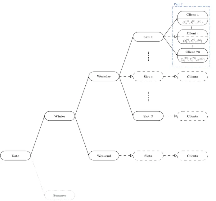
Chapter 2 reviews the existing residential energy consumption modeling approaches and lists the previous work on the electric water heating load model. Chapter 3 explains the different scenarios developed in this study and describes the approach for determining the general time segmentation. Chapter 4 presents the methodology of parameter estimation for the three features. Chapter 5 shows how the typical pattern of sub-populations are found through clustering on these features in every time period. The architecture of the methodology in this project is illustrated in Figure 3.2 and Figure 5.1.
CHAPTER 2 LITERATURE REVIEW
In this chapter, we first review the main existing techniques for modeling the residential energy consumption in section 2.1 and then take a look at the Markov chain and the electric water heating load model in section 2.2.
2.1 Overview of residential energy consumption modeling approaches
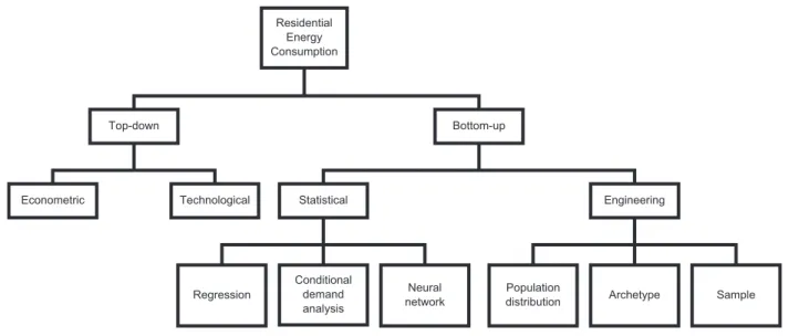
Renewable energy has attracted much attention over the past decade. During that period, the subject has been extensively explored, and it is still under investigation both in its methodological aspects as well as in energy management applications. A significant number of studies has been devoted to the study of end-use energy on the basis of data collection in the residential sector, for different types of electric loads. In this thesis, our main focus is on the literature related to hot water consumption in electric water heaters (EWH’s) given that the emphasis of the smartDESC project of which this research has been a part, has been on learning how to use EWH’s as effective batteries. Indeed, EWH’s can both help store excess generated power, and contribute to load relief in times of generation deficit by deferring temporarily their own electricity consumption. Although the research background and the consumption categories (water or electricity) may be different, previous studies can be valuable sources of ideas in data management, analysis and data based statistical model building. In this section, we provide an overview of residential end-use energy consumption modeling approaches. Figure 2.1 presents the main existing modeling methods while Table 2.1 lists perceived positive and negative attributes.
2.1.1 Top-down approach
In the top-down approach, the residential sector is regarded as an energy sink, and the individual end-uses details are neglected. Parti and Parti (1980) point out that the number of occupants, electricity price and household income are the three variables which have an effect on the energy consumption related to hot water extraction. The input variables in top-down models usually are the macroeconomic factors (e.g. GDP1, income, pricing policies),
climate-related effects, the number of units of residences (Swan and Ugursal, 2009). These common and widely available variables as well as the historical consumption data are usually used to build one or several equations. Therefore, the residential sector energy needs can be
Figure 2.1 Top-down and bottom-up modeling techniques for estimating the regional or national residential energy consumption (Swan and Ugursal, 2009).
estimated approximately. Top-down models fall mainly into two groups: econometric and technological.
Econometric models use mostly the economic factors, such as price and income, as variables. Bentzen and Engsted (2001) proposed and tested Denmark annual energy consumption re-gression models, which related to only three variables: income, energy price, and heating degree days (HDD2).
Technological models use the overall number of residences and the appliance ownership level and average power rating. Zhang (2004) developed the regression equations of unit energy consumption (UEC3) using HDD for China, Japan, the United States and Canada
respec-tively and also studied the potential trend of consumption of different types of source of energy.
In top-down approaches, one uses only aggregate energy consumption data, together with a set of relevant macroeconomic indicators, to produce regression models ultimately used for planning purposes. However, their main shortcoming lies in the absence of individual detailed information which prevents a study of the characteristics of typical sub-populations. More-over, the model is not sensitive to technological advances or sudden housing stock changes, since the regressions are based on the historical consumption information (Swan and Ugursal,
2Heating degree day: the number of degrees that a day’s average temperature is below 18◦C, the
temper-ature below which buildings need to be heated.
2009).
2.1.2 Bottom-up approach
In bottom-up approaches, model building starts with an observation of specific end-usages in a set of dwellings, representative of typical populations. Global behaviour is sub-sequently obtained by aggregating individual dynamics. While more intensive in terms of data collection than top-down approaches, bottom-up approaches can provide load type spe-cific information, as well as aggregate dynamics at substation, regional or national levels depending on the types of applications intended for the models.
Given that the level of details of individual information studied can vary vastly from one dataset to another, the techniques that permit maximum information extraction from the available data also may vary. The so-called bottom-up statistical and bottom-up engineering are the ones most discussed in the literature. When estimating consumption, the former method is based mainly on historical data, while the latter tends to rely on engineering based knowledge of household appliances, namely their types, power ratings and even the heat transfer characteristics.
Bottom-up engineering model
There are two essential strengths in bottom-up engineering models: (i) ability to reflect technological upgrades and (ii) a much weaker dependence on historical consumption data. Indeed, estimates of energy consumption are obtained by forming the product of expected local consumption as derived from power rating, usage frequency (related to number of members in the household), energy efficiency, heat transfer effect, etc, and the number of houses. When a local technological upgrade occurs (e.g. replacement of heating supply facilities), the engineering model is able to update immediately the new regional and national consumption estimation by simply switching the technological characteristics to the new value. At the “bottom” level, three techniques appear to be predominantly used to capture users variability:
The distribution technique uses distributions to represent the appliance ownership among houses and usually picks deterministic averages as characteristics values (Capasso et al., 1994; Kadian et al., 2007).
The archetype technique classifies the houses into several categories according to their sizes, year and facilities. Subsequently, the “top” level regional and national consumption is ob-tained as the sum of the products of number of houses in each category and the energy
con-sumption dynamics of the most typical one, also called archetype, in that category (Huang and Brodrick, 2000).
Finally, the sample technique requires the development of a large representative housing energy consumption database to carry out the calculation (Fung et al., 2001).
Although engineering based model building approaches start from the microscopic level us-ing housus-ing stock information, they cannot specify occupants’ behaviour pattern in every household. This limitation is precisely due to the fact that engineering-based methods tend to ignore historical consumption data.
Bottom-up statistical model
Statistical model building approaches, which invariably require a large end-use survey sample, are obtained by building individual user models, first including dependency on one or more indicator variables. Such models are essential to retrieve the end-user’s behaviour in simu-lation and estimation. Three model categories are considered, namely polynomial regression models, neural networks and conditional demand models.
Regression models remain the traditional concept. Energy consumption is expressed in terms of a number of observable variables that may have an influence. A variable selection step is sometimes required to simplify and improve the model.
Neural network techniques build a fully computational model. The parameters involved in that nonlinear modeling strategy do not possess any particular physical significance. The neural network consists first of a layer of input variables, then multiple subsequent hidden layers of neurons and a last layer of output energy consumption. A neuron’s function is a sum of weighted functions of the neurons in the previous layer. Given a series of observed input/output sequences, the neural network parameters are adjusted by minimization of the output error based on the input of the sequences in the training data set. Aydinalp et al. (2004) developed two neural network based models to estimate the space heating and domestic hot water energy consumptions in the Canadian residential sector. Using the technique presented by Yang et al. (2005) the coefficients and bias in a previously trained network could be continuously updated as new information.
Conditional demand analysis (CDA) techniques rely on the appliance activity record and time-based energy billing data. It quantifies the appliance demand to binary (ON and OFF) or multi-level power rating state. Combined with the energy billing data, it is even possible to study the behaviour pattern for arbitrary appliances and their energy consumption activity. This technique is of particular interest for our research since the electric water heater demand
in this thesis is assumed to be of binary type (either ON or OFF).
Johnson et al. (2014) presented a bottom-up statistical method for modeling household oc-cupant behaviour to simulate residential energy consumption, using a dataset gathered by the U.S. Census Bureau in the American Time Use Survey (ATUS, 2003-2011). The lat-ter defined ten different activities (sleeping, grooming, laundry, food preparation, washing dishes, watching television, using computer, non-power activity, away, away for travelling) as the human behaviour options for the survey and recorded the activity start and stop time based on up to one minute resolution for a total of 124,517 respondents. A Markov chain model was built for each by determining statistically the transition probabilities from one state (or activity) to another at given time t based on the high-resolution data. In the aggre-gated version, it mentioned that the Markov chain Monte Carlo simulation method required approximately 100 occupants or 40 households for the simulation to produce a reasonably accurate picture of overall residential activity pattern.
One of the most important differences in the nature of our data set and ATUS’s or data sets in most other studies is the availability of activities’ label information. In the majority of researches, the quantity of consumption at time t is collected along with its activity name or related residential load. So it can be modeled with multi-states (distinct activities), and the technological characteristics and performance of activities or appliances (usually using deterministic averages) are also discussed. We note that this thesis is devoted to discussing how to model hot water extraction by means of only a binary Markov chain (extraction present or not) in view of the fact that no information is available as to the reasons of the observed extraction as in the ATUS data set for example.
ATUS data and our research data share the following common points:
• Both of them employ the concept of quantifying the appliance/activity demand as the states in CDA.
• The secondary activities are not taken into account, i.e. both consider that only one activity is taking place on any active time interval.
Indeed, if the combinations of activities were to be considered, the Markov chain would get more complex, as more situations would have to be taken into consideration, each one being associated with a smaller sample size, and thus with a poorly estimated probability (Johnson et al., 2014). Indeed: N = r X k=0 n! k!(n − k)! (2.1)
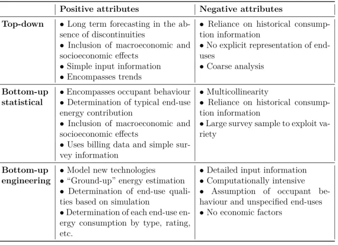
Table 2.1 Perceived positive and negative attributes of the three major residential energy modeling approaches (Swan and Ugursal, 2009).
Positive attributes Negative attributes Top-down • Long term forecasting in the
ab-sence of discontinuities
• Reliance on historical consump-tion informaconsump-tion
• Inclusion of macroeconomic and socioeconomic effects
• No explicit representation of end-uses
• Simple input information • Coarse analysis • Encompasses trends
Bottom-up • Encompasses occupant behaviour • Multicollinearity statistical • Determination of typical end-use
energy contribution
• Reliance on historical consump-tion informaconsump-tion
• Inclusion of macroeconomic and socioeconomic effects
• Large survey sample to exploit va-riety
• Uses billing data and simple sur-vey information
Bottom-up • Model new technologies • Detailed input information engineering • “Ground-up” energy estimation • Computationally intensive
• Determination of end-use quali-ties based on simulation
• Assumption of occupant be-haviour and unspecified end-uses • Determination of each end-use
en-ergy consumption by type, rating, etc.
• No economic factors
where N the necessary number of states of Markov chain, r the number of activities allowed to take place simultaneously, n the total number of distinct activity types.
At this stage, let us note that the modeling approach adopted in our thesis will draw on both statistical (in particular CDA) and engineering (both archetype and sample) bottom-up modeling approaches, in order to segregate consumers present in our data set into the sub-population classes most relevant for the goals of the smartDESC project, i.e. the coordi-nation of distributed storage for mitigating generation variability introduced by intermittent renewable energy sources in power systems.
2.2 Markov chain and electric water heating load model
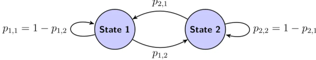
A Markov chain (MC) is a stochastic process of a particular type. The crucial defining property of Markov chains and which accounts for their wide usage as a tractable stochastic model is memoryless i.e., in the case of a discrete time MC, the property that the probability
of moving to different states at time t + 1 conditional on the state at time t , is independent of all the states that were visited before t (see Lefebvre (2005) for example). As a result, at any time t, one can unambiguously define a matrix of probabilities of transitioning between any two states; it is called the transition probability matrix, and it fully characterizes the future probabilistic evolution of a MC, given its most current state.
Thus, assuming S is the state space of a MC of dimension k, the transition matrix Pt is
generated in time series of dimension k × k with the probabilities pi,j = Pr(Xt+1= j|Xt= i)
(i.e. the probability of going from state i to state j.). More specifically:
Pt = p1,1 · · · p1,k .. . . .. ... pk,1 · · · pk,k k X j=1 pi,j = 1 ∀i = 1, 2 . . . , k (2.2)
The same information can also be represented by the transition graph. Figure 2.2 is a transition graph of a two-state MC with each state drawn as a circle and the transition probability pi,j drawn as an arrow between states.
State 1 State 2 p2,2 = 1 − p2,1
p2,1
p1,1 = 1 − p1,2
p1,2
Figure 2.2 Transition graph of a two-state Markov chain.
The elemental electric water heating load model was originally proposed in Chong and Debs (1979). The dynamics in a water heater tank was modeled by using physical thermal charac-teristics, ambient temperature, inlet/outlet water temperature, state of thermostat control, state of load management control and customer-driven hot water demand. However, the customer-driven hot water withdrawal profile is a non-stationary random process, which is hard to simulate (Kempton, 1988; Alvarez et al., 1992).
Based on the Chong and Debs physically-based elemental stochastic electric water heating load model, Malhamé (1990), and Laurent and Malhamé (1994) have shown how the ideas of statistical mechanics could be used to derive a partial differential equation model of the aggregate behaviour of a large number of identical such loads. Three archetypal households of different physical and consumption parameters were discussed in Laurent et al. (1995). In our research, a two-state MC model is used to simulate the hot water withdrawal profile at the individual device level. The model is described in detail at the beginning of Chapter 4.
Using the ON-OFF two-state MC model, the demand process can also be seen as an alter-nating 0-1 renewal process with the water extraction rate a constant. Under the assumption that the processes are time homogeneous stationary, El-Férik and Malhamé (1994) devel-oped a methodology to identify the model parameters from the statistical consumption data using the Laplace transform expressions of moments of total occupation time over fixed time windows. Indeed, power company billing is based on measurements of energy consumption data over appropriate fixed length successive time intervals. These fixed-length time intervals were interpreted as the combinations of water heater busy time durations (i.e. with hot wa-ter demand present) and that of silent time durations (with no hot wawa-ter demand). If wawa-ter extraction, when present, is considered to occur at a constant rate, one can then claim that the total energy extraction is proportional to the total busy time over the fixed interval. The Laplace transform expressions of moments are used in Chapter 4 to establish the equations for estimating the three EWH MC parameters over a given time zone of homogeneous time invariant parameters.
CHAPTER 3 TIME SEGMENTATION
In this chapter, we define different scenarios and cases to study and select the general time segmentation structure, which will be used in the subsequent stage of parameter estimation. Figure 3.2 helps to understand the structure of this chapter, except that the last column is about Chapter 4.
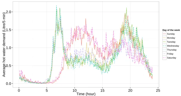
3.1 Weekday/Weekend scenarios
The average plots of hot water consumed, against time in distinct days of a week from Sunday to Saturday, are shown in Figure 3.1. As one can observe from the plots, hot water consumptions on weekdays are significantly different from those on weekends and this result agrees with most people’s lifestyles. On weekdays most of the hot water is consumed during two peak periods, in the early morning and in the evening, because consumers are absent or sleeping for the rest of the time. On weekends instead, people tend to get up later, which means starting to use hot water later, and people tend to stay at home longer, which leads to higher water consumption than weekdays. To get a more accurate model, we thus have to
0.0 0.5 1.0 1.5 2.0 0 5 10 15 20 25 Time (hour) A v er age hot w
ater demand (Litre/5 min)
Day of the week Sunday Monday Tuesday Wednesday Thursday Friday Saturday
Figure 3.2 Methodology diagram part 1. Starting with the raw dataset, each node represents a subcase defined by a different criterion and the dashed line nodes means there are multiple cases. The directions of the arrows point to the subdivided cases.
deal with the data in weekdays and the data in weekends separately, and these two scenarios are considered in this project. Moreover, the same algorithm and simulation methods are applied to both weekday and weekend scenarios, the only difference being the input data. The consumption patterns are also expected to vary from one season to the other, particu-larly for the cities like Montreal with very cold winters, and occasionally very hot summers. Indeed, the temperature is also an important factor affecting people’s hot water consumption behaviour. For example, when it gets warmer, people usually tend to take a shorter shower with less hot water, which means there is less energy consumption. There are long summers (from May to October) and long winters (from November to April) in Quebec. The dataset used in this project only contains data from November to April. In other words, if we were to continue gathering data during summer time, we would need to further elaborate the model by setting up four scenarios corresponding to weekday/weekend in summer/winter.
3.2 Time period (slot) division
Note that a time inhomogeneous modeling problem is dealt with in this thesis and this property has to be captured in our models. Different distributions are needed to represent the consumption in different periods of time. According to the observed data, most clients maintain similar peak consumption times from day to day, thus leading us to an assumption of 24 hour periodicities related to general human activities. An inhomogeneous but of 24 hour period behavioural model is then broken up into several homogeneous modeling problems. In order to define the different time slots, we introduce one-dimensional fused lasso (Tibshi-rani et al., 2011).
3.2.1 One-dimensional fused lasso approach
This section is an introduction about the lasso problems. We start with a minimization problem (3.1) whose result is in the form of soft-thresholding (3.4). It is found that problem (3.1) is somehow equivalent to the common lasso problem (3.5). Then, we specify the one dimensional fused lasso approach and relate it to our case.
Soft-thresholding helps to solve the following optimization problem where both the Euclidean and the absolute value norms are involved
argmin
β∈Rn
ky − βk22 + λ kβk1 (3.1)
is a function of parameter λ. (3.1) can also be written as argmin n X i=1 (yi− βi)2+ λ|βi| (3.2)
The sum is minimized whenever one minimizes every component quadratic function of βi in
the sum. The extremum of the function f (x) = (b − x)2+ λ|x| is at x = b − λsign(x)/2. By
discussing different conditions of sign of x, values of b, λ/2 and f (0), the solution of f (x) turns out to be argmin f (x) = b + λ/2 if b < −λ/2 0 if b ≤ |λ|/2 b − λ/2 if b > λ/2 (3.3)
It is in a form of soft-thresholding, if we denote b as the variable and λ/2 as the threshold value. Hence the solution to problem (3.1) for each coordinate i = 1, . . . , n is
ˆ βi = soft(yi, λ/2) = yi+ λ/2 if yi < −λ/2 0 if yi ≤ |λ|/2 yi− λ/2 if yi > λ/2 (3.4)
where soft(·, ·) is the notation of soft-thresholding and Figure 3.3 shows the function. It is shown that soft-thresholding sets small values ∈ [−λ/2, λ/2] to zero while all others are biased. yi βi −λ 2 λ 2
Figure 3.3 Soft-thresholding function. The red line reprsents function βi = soft(yi, λ/2),
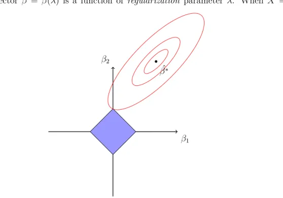
The lasso problem is commonly written as ˆ β = argmin β∈Rp 1 2ky − Xβk 2 2+ λ kβk1 (3.5)
where y ∈ Rn is a response vector, X ∈ Rn×p is a matrix of predictors and λ ≥ 0. The coefficient vector ˆβ = ˆβ(λ) is a function of regularization parameter λ. When X = In×n,
β1
β2
ˆ β∗
Figure 3.4 Estimation picture for the lasso (p = 2). The solid blue area is the `1 penalty
term shown as the constraint region, while the red ellipses are the common residual sum of squares (RSS) contours with ˆβ∗ the RSS coefficients. The solution is the first place the RSS
contours hit the constraint region.
(3.5) is called signal approximation case and can be rewritten as
argmin β∈Rn 1 2ky − βk 2 2+ λ kβk1 = argmin 1 2 n X i=1 (yi− βi)2+ λ|βi| (3.6) = argmin n X i=1 (yi− βi)2+ 2λ|βi| (3.7)
(3.2) and (3.7) share similar form and the solution of (3.7) is soft(yi, λ). Figure 3.4 also shows
geometrically why the lasso encourages sparse solutions: there are sharp edges and corners for the blue area because of the absolute value in `1 norm and it is highly likely that the
contour will first hit the corner, then some of the coefficients will be set to zero. Hence, the lasso performs shrinkage and subset selection.
Now if the lasso problem (3.5) is generalized to ˆ β = argmin β∈Rn 1 2ky − Xβk 2 2+ λ kDβk1 (3.8)
where D ∈ Rm×p is a penalty matrix. If X = I and D is specified as the (n − 1) × n matrix of first differences given in (3.9), it is called the one-dimensional fused lasso (1d fused lasso) problem. D = −1 1 0 · · · 0 0 0 −1 1 · · · 0 0 .. . ... ... . .. ... ... 0 0 0 · · · −1 1 (3.9)
As X = I is full column rank, the solution is ˆ β = y − D>uˆ (3.10) and ˆ u = argmin u∈Rn−1
||y − D>u||22 subject to ||u||∞ ≤ λ (3.11)
Furthermore, for each coordinate i = 1, . . . , n − 1
ˆ ui ∈ {−λ} if βi+1− βi < 0 [−λ, +λ] if βi+1− βi = 0 {+λ} if βi+1− βi > 0 (3.12)
(Arnold and Tibshirani; Tibshirani et al., 2011)
The 1d fused lasso is the common signal approximator case and is used in settings where coordinates in the true model are closely related to their neighbours. Recall the idea of breaking up the inhomogeneous 24 hour period behavioural model into several homogeneous modeling problems. If we take n = 288 (see data structure in Section 1.1) and the response vector y ∈ Rn as the consumption sequence Z = {Z1, Z2, . . . , Z288}. Zi is the volume of
hot water consumed during the i-th 5 min of one day (i = 1, 2, . . . , 288). The problem is of 1-dimensional structure and its coordinates are the i-th unit time corresponding to successive
positions on a straight line. The expression of 1d fused lasso becomes ˆ β = argmin β∈Rn 1 2 288 X i=1 (Zi− βi)2+ λ 288−1 X i=1 |βi+1− βi| (3.13)
The consumption sequence Z is generated from a process whose mean changes at only a smaller number of locations, which implies different human activity time periods. So the 1d fused lasso aims to find a piecewise constant vector β of model coefficients fitting well to consumption sequence Z and the subset selection is the coordinates of changes of β, which indicate the edges of time periods.
Indeed, ˆβ is a function of λ. The `1 norm penalizes the absolute differences in adjacent
coordinates of β. The choice of cost function (3.13) for the segmentation problem, and the role of the lambda coefficient are best understood by considering two limiting cases:
(i) If λ = 0, (3.13) equals to argminP288
i=1(Zi− βi)2, so ˆβ is identical with Z. The fitting is
perfect but makes no sense, because every data point would define a separate interval. (ii) If λ approaches infinity, (3.13) is equivalent to argminP288
i=1(Zi− βconst)2, where |βi+1−
βi| = 0 and ˆβ becomes a constant vector. The best fit is βconst =P288i=1Zi/288, and all
the coefficients become equal to the mean consumption. The 288 degrees of freedom shrink to a single degree of freedom.
So tuning the regularization parameter λ for the 1d fused lasso problem is actually a com-promise between accuracy of fit and number of changes between successive values of β. The crucial point of this method is to choose an appropriate regularization parameter λ. The paragraph “record λobs” in section 3.2.2 presents how we choose λ for each client. However, contrary to expectation, it is very hard to take this decision directly and work has to be repeated when the sequences change. The cross-validation (Geisser, 1993; Kohavi, 1995; Devijver and Kittler, 1982) is an often used method to automate the choice of ˆλ. However, when the number of clients increases, there are a larger number of sequences to deal with, and more ˆλ have to be chosen. It would be computationally expensive to use cross-validation every time. So a linear regression model is suggested here rather than the cross-validation. More precisely, in view that larger variance means one needs more effort on trend filtering, and thus λ leading to desirable results has to be higher, we conjecture a linear model relating an “adequate” choice of λ to the standard deviation σ of water consumption over the time slot one has to segment. The linear function parameters will be estimated from a regression analysis based on a preliminary “manual tuning” of λ for a series of examples from some
training set. With σ easily computed from the raw data, this approach can lead to an automation of the choice of ˆλ.
So in the following sections, we present our method to automate the selection of the λ coefficient in the performance criterion. As mentioned above, the strategy is to develop an empirical linear relation between σ and λ and test the resulting performance. First, we separate the data into a training set and a test set. The elements in each of the sets are then separated according to their σ; we choose λ visually (manual tuning) for each client (Section 3.2.2). The training set is used to obtain an empirical λ-σ function using linear regression and the test set is subsequently used to evaluate the quality of the time segmentation based on the empirical function obtained. Once the function is defined as acceptable, the linear equation λ = α1σ + α0 is used to determine the proper time segmentation for each client
(Section 3.2.3).
3.2.2 Training and test sets preparation Standard deviation
For each client j, ˆσj is defined as
ˆ σj = q V[Zj] , v u u t 1 288 − 1 288 X j=1 (Zji− ¯Zj)2 (3.14)
where j is the client tag (1 ∼ 73). We call i the time index (1∼288). Its maximal value 288 comes from the total number of 5 min unit time per day: 24 h/day × 60 min/h ÷ 5 min = 288/day. Zij represents the average consumption of client j during the i-th 5 min time unit
of 24 hours, Zj = {Zj1, Zj2, . . . , Zj288} and ¯Zj = 2881 P288i=1Zji.
Figure 3.5 shows 73 clients’ standard deviation σj of average consumption every 5 min in
weekday and weekend scenarios respectively and the decision of forming training set and test set.
Record λobs
In the fused lasso approach, values of the regularization parameter λ must be chosen for the various customers. This choice is highly dependent on personal discernment. For each client j, several different λ should be tested until we judge the result to be “suitable” and record it as observed value λobs
j .
Figure 3.6 takes client 5 as an example and λobs
0 10 20 30 40 50 60 70 0 .5 1 .0 1 .5 2 .0
rank sorted by standard deviation
st a n d a rd d e vi a ti o n (a) 0 10 20 30 40 50 60 70 0 .5 1 .0 1 .5
rank sorted by standard deviation
st a n d a rd d e vi a ti o n (b)
Figure 3.5 Rank sorted by σ2 (a) weekday (b) weekend. There are 73 clients’ standard
devi-ation σj of average consumption every 5 min in weekday and weekend scenarios respectively.
y-axis is standard deviation σj. x-axis represents their rank according to size among 73
clients. The red lines cross the points that are selected to form a test set with a quantity of 13 in each scenario. As the total number of clients is 73, we choose rank 5, 10, 15, 20, 25, 30, 35, 40, 45, 50, 55, 60, 65. The remaining 60 samples form the training set.
of regularization parameter. There are some characteristics: two peak times present in the morning and evening, low consumption between them and silence during night time.
The black line represents the smoothed signal ˆβ from the 1d fused lasso (3.13). According to (3.10), (3.11) and (3.12), the coefficients are soft-thresholded on difference of adjacent β, so we note this piecewise constant βbiased. The time periods are separated by the red vertical
lines, where βi+1 6= βi. The blue dashed line, called βunbiased represents the mean of data
whose βbiased maintain the same value. It helps to visualize the consumption trend between
successive time periods.
The detected positions of changes of β (red) are sometimes consecutive, especially when λ is small. The reason is that there is a gradual increase (decrease) of demand during that period. If we segment a slot containing gradual increase (decrease) demands, it will not be a stationary slot. So λobs should help decide separate successive regions but be such that the
least number of very short slots are detected.
This work is repeated for every client j and we record its λobs
j . Table 3.1 lists the results
0 50 100 150 200 250 0 1 2 3 4 5 6
lambda=9.5 tested for client 5
time index a ve ra g e co n su mp ti o n (L /5 mi n )
Figure 3.6 Example: λobs
5 = 9.5 for client 5. x-axis indicates the sequence number i of unit
time 5 min. The black dots represent the average consumption Z5i observed from the data.
The black line shows the piecewise constant βbiased while the blue dash line is βunbiased. The
red dash lines indicate the time period (slot) segmentation.
Table 3.1 Table of weekday test set.
No. Client tag j Rank Standard deviation σ λobsj
1 18 5 0.3 2 2 20 10 0.4 3.1 3 3 15 0.5 3.7 4 73 20 0.6 5.6 5 46 25 0.7 7.8 6 53 30 0.7 7.7 7 22 35 0.8 3.3 8 5 40 0.9 9.5 9 29 45 1.0 11.1 10 14 50 1.1 6.1 11 63 55 1.2 12.4 12 48 60 1.4 14.5 13 34 65 1.6 19.1
3.2.3 Regression model
A linear regression for the choice of ˆλ is preferable to cross-validation in this case. Because when the number of clients increases, it would be computationally expensive to use cross-validation every time. Moreover, larger variance σ2 means one needs more effort on trend filtering, and thus λ leading to desirable results has to be higher. We conjecture a linear model relating the choice of ˆλ to the standard deviation σ of water consumption over the time slot one has to segment. With σ easily computed from the raw data, this approach can lead to an automation of the choice of ˆλ. Also, the linear relation is postulated between λ and the standard deviation σ, not the variance σ2, because λ and σ have the same scale.
We now study the linear relationship between σ and λ. For that purpose, there is no need to segregate between weekday samples and weekend samples. Therefore, we take the union of weekday and weekend training/test sets as our final training/test set in this linear regression model study.
Model discussion
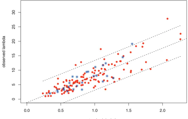
Figure 3.7 shows “observed” value λ versus sample standard deviation. The linear regression model is in the form of λ = α1σ + αˆ 0 with α1, α0 constant. As we use sample standard
deviation ˆσ, not standard deviation σ, λ should also be replaced by its estimate ˆλ. Then the following relation is obtained.
ˆ
λ = 9.4ˆσ − 1.2 (3.15)
Table 3.2 summarizes the results of our example linear regression as well as the R2 indicator
(0.714 a good fit) with a p-value 0.001 (close to zero). The coefficient of determination R2 is
expressed as the ratio of the explained variance to the total variance (Gujarati, 2009). The explained variance is the variance of the model predictions, while the sample variance is the variance of the dependent variable.
R2 = SSreg SStot = SSreg/n SStot/n (3.16) where ¯y = n1Pn
i=1yi mean of observed data, SStot = Pi(yi − ¯y)2 total sum of squares and
0.0 0.5 1.0 1.5 2.0 0 5 1 0 1 5 2 0 2 5 3 0 standard deviation o b se rv e d l a mb d a
Figure 3.7 Linear regression model. The training set (60 × 2 = 120 points) is plotted in red and the test set (13 × 2 = 26 points) in blue. Note that the blue dots are obtained using independent observations. The three dashed lines are the model obtained ˆλ = 9.4ˆσ − 1.2, together with the 95% lower and upper confidence bounds. The confidence bounds cover the majority of cases.
Model-based auto-selected λ plotting
This section presents the 73 clients’ slot cut visualization. They are Figure 3.8: Weekday auto-selected λ model
Figure 3.9: Weekday λobs defined slot cut
Figure 3.10: Weekend auto-selected λ model Figure 3.11: Weekend λobs defined slot cut
In the top figures on each page, the black and white colors show different slot cut decided by 1d fused lasso, where their regularization parameters ˆλj are computed from sample standard
deviations sigmaj and equation (3.15) for Figure 3.8 and Figure 3.10 or visually decided λobs
for Figure 3.9 and Figure 3.11. Every client has the piece-wise constant vector βunbiased, the edge points of regions are the changing positions from black to white.
Table 3.2 Summary of the linear regression model λ = α0 + α1σ.
Dependent variable: λ
Sample standard deviation ˆσ 9.389∗∗∗ (0.548) Constant −1.154∗∗ (0.562) Observations 120 R2 0.714 Adjusted R2 0.711 Residual Std. Error 2.581 (df = 118) F Statistic 293.901∗∗∗ (df = 1; 118) Note: ∗p<0.1;∗∗p<0.05;∗∗∗p<0.01 Discussion of results
Our analysis of the results shown in Figure 3.8, Figure 3.9, Figure 3.10, and Figure 3.11 can be summarized in the following two points:
• The auto-selected λ method offers a satisfactory result.
In both of the weekday and weekend scenarios, the model based results (Figure 3.8 and Figure 3.10) concur with the results of λobs (Figure 3.9 and Figure 3.11), most notably in the high similarity between their bar-plots. So our proposed method is verified through this experimental model. Thus, compared with the repeated work of tuning visually λobs for every
sample, if the linear model is well trained, the automatic λ selection method is a much faster and much more convenient way of achieving a good segmentation result, since the standard deviation of data is easy to calculate. If there is a large number of samples to deal with in the future, it is advised to use this method.
• A general segmentation structure should be selected.
It is important to remember that modeling effort is aimed at the general objectives of: (i) clustering customers into classes within which consumption patterns are relatively homo-geneous; (ii) identifying for each class, the distribution of piecewise constant parameters characterizing the water demand assumed, as we shall see, to evolve according to two-state
Markov chains. In particular, short time intervals (less than 2 hours) are avoided. This is because, in view of the rarity of samples on short intervals, it would be impossible to obtain consistent estimates of the process parameters (estimation is discussed in the next chapter). Also, since we shall see lag 1 autocovariance function empirical estimates are used in the parameter estimation part, sufficiently long time intervals are needed to empirically estimate the value (see equation (4.18) in Section 4.3).
For that purpose, and based on our customer wise time segmentation results, we have to extract common time periods within which a large number of customers are assumed to behave with stationary water consumption statistics. So the boundary points should be set where the majority of clients are changing their consumption pattern. Our analysis of Figure 3.8, Figure 3.9, Figure 3.10, and Figure 3.11 suggest the following time slot sequence of boundary points:
1. weekday time slot boundary points: 72, 96, 156, 216, 264, 288 2. weekend time slot boundary points: 84, 120, 156, 216, 264, 288
This segmentation preserve the intuition of the presence of a silent sleeping time, a morning peak period, a low consumption period, an evening peak period, followed by a quieter early night period.
Table 3.3 Time segmentation for homogeneous water demand statistics. Slot No. Time interval
Weekday Weekend 1 0∼6h 0∼7h 2 6∼8h 7∼10h 3 8∼13h 10∼13h 4 13∼18h 13∼18h 5 18∼22h 18∼22h 6 22∼24h 22∼24h
1 2 3 4 5 6 7 8 9 10 11 12 13 14 15 16 17 18 19 20 21 22 23 24 25 26 27 28 29 30 31 32 33 34 35 36 37 38 39 40 41 42 43 44 45 46 47 48 49 50 51 52 53 54 55 56 57 58 59 60 61 62 63 64 65 66 67 68 69 70 71 72 73 0 12 24 36 48 60 72 84 96 108 120 132 144 156 168 180 192 204 216 228 240 252 264 276 288 time index T a g 0 5 10 15 20 0 12 24 36 48 60 72 84 96 108 120 132 144 156 168 180 192 204 216 228 240 252 264 276 288 time index co u n t
Figure 3.8 Weekday auto-selected λ model. Top panel: x-axis is time sequence number from 1 to 288 (5 min per unit). y-axis is client tag from 1 to 73. For a client y, when the color changes at time index x, it means this client’s consumption pattern is changing and we are moving to a new slot. Conversely, when the color remains the same, it means the process is considered to have a relatively stationary property, indicating that parameter estimation theory based on this stochastic assumption is applicable. Bottom panel: The bar-plot indicates how many clients possess a slot cut point at time index x.
1 2 3 4 5 6 7 8 9 10 11 12 13 14 15 16 17 18 19 20 21 22 23 24 25 26 27 28 29 30 31 32 33 34 35 36 37 38 39 40 41 42 43 44 45 46 47 48 49 50 51 52 53 54 55 56 57 58 59 60 61 62 63 64 65 66 67 68 69 70 71 72 73 0 12 24 36 48 60 72 84 96 108 120 132 144 156 168 180 192 204 216 228 240 252 264 276 288 time index T a g 0 5 10 15 20 0 12 24 36 48 60 72 84 96 108 120 132 144 156 168 180 192 204 216 228 240 252 264 276 288 time index co u n t
Figure 3.9 Weekday λobs defined slot cut. Top panel: x-axis is time sequence number from 1
to 288 (5 min per unit). y-axis is client tag from 1 to 73. For a client y, when the color changes at time index x, it means this client’s consumption pattern is changing and we are moving to a new slot. Conversely, when the color remains the same, it means the process is considered to have a relatively stationary property, indicating that parameter estimation theory based on this stochastic assumption is applicable. Bottom panel: The bar-plot indicates how many clients possess a slot cut point at time index x.
1 2 3 4 5 6 7 8 9 10 11 12 13 14 15 16 17 18 19 20 21 22 23 24 25 26 27 28 29 30 31 32 33 34 35 36 37 38 39 40 41 42 43 44 45 46 47 48 49 50 51 52 53 54 55 56 57 58 59 60 61 62 63 64 65 66 67 68 69 70 71 72 73 0 12 24 36 48 60 72 84 96 108 120 132 144 156 168 180 192 204 216 228 240 252 264 276 288 time index T a g 0 5 10 15 0 12 24 36 48 60 72 84 96 108 120 132 144 156 168 180 192 204 216 228 240 252 264 276 288 time index co u n t
Figure 3.10 Weekend auto-selected λ model. Top panel: x-axis is time sequence number from 1 to 288 (5 min per unit). y-axis is client tag from 1 to 73. For a client y, when the color changes at time index x, it means this client’s consumption pattern is changing and we are moving to a new slot. Conversely, when the color remains the same, it means the process is considered to have a relatively stationary property, indicating that parameter estimation theory based on this stochastic assumption is applicable. Bottom panel: The bar-plot indicates how many clients possess a slot cut point at time index x.
1 2 3 4 5 6 7 8 9 10 11 12 13 14 15 16 17 18 19 20 21 22 23 24 25 26 27 28 29 30 31 32 33 34 35 36 37 38 39 40 41 42 43 44 45 46 47 48 49 50 51 52 53 54 55 56 57 58 59 60 61 62 63 64 65 66 67 68 69 70 71 72 73 0 12 24 36 48 60 72 84 96 108 120 132 144 156 168 180 192 204 216 228 240 252 264 276 288 time index T a g 0 5 10 15 0 12 24 36 48 60 72 84 96 108 120 132 144 156 168 180 192 204 216 228 240 252 264 276 288 time index co u n t
Figure 3.11 Weekend λobs defined slot cut. Top panel: x-axis is time sequence number from 1
to 288 (5 min per unit). y-axis is client tag from 1 to 73. For a client y, when the color changes at time index x, it means this client’s consumption pattern is changing and we are moving to a new slot. Conversely, when the color remains the same, it means the process is considered to have a relatively stationary property, indicating that parameter estimation theory based on this stochastic assumption is applicable. Bottom panel: The bar-plot indicates how many clients possess a slot cut point at time index x.
CHAPTER 4 PARAMETER ESTIMATION
We have 73 customers’ data in total. This section mainly presents the derivation of the method, which was used to estimate the water demand Markov chain time segment parame-ters for every single client on each defined time segment in Table 3.3. Indeed, the distribution of a hot water consumption event time durations was found to approximately follow an ex-ponential distribution; and while off consumption periods may not be exex-ponential, we find it analytically convenient to work with a two-state Markov chain water demand model.
ON
OFF
1 − β(t)β(t) = λ0e−λ0t
1 − α(t)
α(t) = λ1e−λ1t
Figure 4.1 Two state Markov chain.
Figure 4.1 illustrates a two-state Markov model, where α and β are the transition proba-bilities from state “ON” to state “OFF” and from state “OFF” to state “ON” over time duration t. In this specified model, state “ON” (also called state 1) means consumption is present; its transition probability α(t) is the exponential distribution with rate λ1, while state
“OFF” means no consumption and is denoted state 0. Its transition probability is exponential with rate λ0. Since in Section 3.2.3, a general slot segmentation has been decided, the
non-stationary 24 hours process is divided into 6 time regions. It is assumed that consumption patterns are stationary within each of them. Therefore, the theory of stationary alternating renewal processes will be later applied to estimate from the data a triplet of constant pa-rameters: “OFF” event rate λ0 (/min), “ON” event rate λ1 (/min) and average extraction
rate c (L/min). Over each time homogeneous interval, the stochastic water demand process will be characterized by these three parameters, and three independent equations will need to be identified based on existing data to estimate these parameters. We choose to obtain these equations through a moment approach (El-Férik and Malhamé, 1994; Mortensen, 1990) with the following moments used: mean, variance, and autocovariance function at lag 1 (i.e. correlation between two successive measurements).
4.1 Alternating renewal process
Let w(t) denote the continuous time alternating 1-0 renewal process of interest at time t with f1(τ ) and f0(τ ) the associated “ON” and “OFF” time durations stationary probability
density functions (pdf’s). Let µi = R0∞τ fi(τ )dτ , i = 0, 1, be the expected “OFF” and
“ON” durations. Assume that “ON” and “OFF” events duration time follow the exponential distributions. So
fi(t) = λie−λit i = 0, 1 (4.1)
where λi = 1/µi.
Also consider the water extraction rate c (L/min), when on, is a constant. Now the hot water consumption process is z(t) = cw(t) while Z(t) ,Rt
0 z(τ )dτ = c
Rt
0w(τ )dτ = cξ(t) is the total
volume consumed random variable during an interval of length t, and ξ(t) can be referred to as the total busy time during t. Given the fact that available customer data is hot water consumed over successive 5 min intervals, we shall develop expressions for the statistics of Zt
t0 =
Rt0+t
t0 z(τ )dτ , t = 5min, t0 = N t, N = 0, 1, 2, . . ..
4.2 Theoretical results
This section presents the moment method and develops the autocovariance functions under the equilibrium conditions in time domain and frequency domain.
4.2.1 Moments expressions
El-Férik and Malhamé have shown that the moments at stationarity of the Laplace transform of E[ξ(t)n] process for a general alternating renewal process satisfy a relationship recursive
in the power index n. In particular, based on their work, one obtains the following general formula for mean and variance1:
E(eq)s [Z(t)] = µ1c µ0 + µ1 1 s2 (4.2) (E(eq)[Z(t)] = µ 1ct/(µ0+ µ1) as expected) and E(eq)s [Z(t)2] = c2{ µ1 µ0+ µ1 2 s3 − 2 (µ0+ µ1)s4 [1 − F0(s)][1 − F1(s)] [1 − F0(s)F1(s)] } (4.3)
1The superscript(eq)means the expectation is taken under equilibrium. The subscript
smeans the Laplace transform