Aid and Growth
Evidence from Firm-level Data
Lisa Chauvet
∗H´
el`
ene Ehrhart
†October 14, 2014
Abstract
This paper explores the impact of foreign aid on firms growth for a panel of 5,640 firms in 29 developing countries, 11 of which in Africa. Using the World Bank Enterprise Surveys data and controlling for firms fixed effects, we find a positive impact of foreign aid on sales growth. This result is robust to various checks, notably to the instrumentation of aid. We then identify the main infrastructure obstacles to firms growth and examine whether foreign aid contributes to relaxing those constraints. We find that electricity and transport are perceived as important constraints which tend to decrease the growth rate of firms, as well as the utilization of their productive capacity. Evidence on the impact of aid on infrastructure obstacles suggests that total aid and aid to the energy sector tend to decrease electricity obstacles. We also show that transport aid projects, geo-localized at the region level, tend to decrease the transport obstacles.
Keywords: Foreign aid. Firms growth. Infrastructures constraints.
JEL codes: F35, O16, O50
∗(1) IRD, LEDa, DIAL UMR 225, Banque de France, PSL, Universit´e Paris-Dauphine, FERDI. †Banque de France.
We wish to thank Agn`es Dufour for amazing research assistance. We also wish to thank Sanvi Avouyi-Dovi, Antoine Berthou, Bruno Cabrillac, Christian Durand, Patrick Guillaumont, Sylviane Guillaumont Jeanneney, J´erˆome H´ericourt, Luc Jacolin, Katja Michaelowa, Henri Pag`es, Sandra Poncet and Emmanuel Rocher for useful discussions. We also thank the participants of the ABCA and AEL conferences for useful comments. This paper is a product of the Franc Zone and Development Financing Studies Division (COMOZOF) of the Banque de France. It reflects the opinions of the authors and do not necessarily express the views of the Banque de France. The usual disclaimers apply.
1
Introduction
The impact of aid on growth has been highly debated over the last decade, without any consensus emerging. Some authors have argued that aid is effective in spurring economic growth depending on specific charac-teristics of the developing countries such as the quality of their macroeconomic policy (Burnside and Dollar, 2000), their exposure to external shocks (Guillaumont and Chauvet, 2001; Collier and Dehn, 2001), their structural handicaps (Dalgaard et al., 2004). Those studies adopt a cross-country approach and all suffer from similar methodological weaknesses, the endogeneity of aid being poorly addressed. Using a better identification strategy based on a gravity model for bilateral aid flows, Rajan and Subramanian (2008) find hardly no effect of aid on aggregate growth.
In this article, we build on the existing literature on aid effectiveness but rely on more disaggregated data to assess its impact on growth. We examine how aid affects firms growth in a panel of 29 developing countries, using the World Bank Enterprise Surveys (WBES) panel datasets.
Aid may affect firms growth by relieving different constraints faced by firms. Aid to infrastructure and aid for trade may contribute to firms getting a better access to markets. Aid to electrical infrastructure may relax the electricity shortages weighting on their production. Inversely, aid may also induce a loss of competitiveness through a Dutch disease effect, as underlined by Rajan and Subramanian (2011).
To explore the impact of aid on firms growth, we compiled a panel dataset stacking firm-level data from the WBES. It is composed of more than 5,000 firms in 29 countries, for which we have two points in time depending on the years the surveys were conducted. Those firms surveys provide information on the growth rate of sales, but also on various other characteristics of the firms - its ownership, its size, its sector of activity. Among those characteristics, the WBES also provide information on the various obstacles to their activity (infrastructure constraints, financing constraints, legal and institutional constraints). In order to assess the impact of aid on firms growth, we combine this panel of firm-level data with macroeconomic variables such as foreign aid, income per capita, the quality of institutions.
There are various sources of endogeneity in the relationship we intend to estimate. Aid is endogeneous to economic performance since donors allocate aid purposively and are likely to react to countries growth performance. One major advantage of examining the impact of aid on a disaggregated outcome such as firms growth is that it considerably attenuates this source of endogeneity concern. Reverse causality (from firms growth to aid allocation) is much less likely than when looking at aggregate growth. Moreover, stacking panel data for firms has rarely been done for developing economies and also presents important advantages when dealing with the endogeneity of aid. Indeed, firms fixed-effects allow to control for time-invariant
heterogeneity, which may otherwise induce an endogeneity bias. The main source of endogeneity which remains is time-varying unobservable heterogeneity. To fully address the issue of aid endogeneity, we thus instrument aid. Following Rajan and Subramanian (2008) and Tavares (2003), we find an exogenous source of variation of aid in the change of total fiscal revenue of donor countries, weighted by the cultural distance between pairs of donor-receiving countries.
The article is structured as follows. After having presented the relevant literature (Section 2), we describe the model and data (Section 3). The benchmark results and various robustness checks are detailed in Section 4. Section 5 presents indirect evidence for the absence of Dutch disease. In Section 6 we examine the impact of aid on the infrastructure obstacles to firms growth. Finally, Section 7 concludes.
2
Aid effectiveness and the constraints on growth: a review of the
debates
2.1
The impact of aid on growth
A large body of the literature on aid effectiveness has explored the impact of aid on aggregate growth rates at the country-level. Since the work of Burnside and Dollar (2000), a flourishing literature has emerged, examining which recipients’ characteristics may make aid more or less effective in terms of growth. A large array of conditions have been found to influence aid effectiveness: the quality of policy choices (Burnside and Dollar (2000)), geography (Dalgaard et al., 2004), exposure to external shocks (Guillaumont and Chauvet, 2001; Collier and Dehn, 2001), post-conflict situations (Collier and Hoeffler, 2004), characteristics of the elite (Angeles and Neanidis, 2009), and the list is not exhaustive. The exponential number of findings on the conditions that affect the aid-growth relationship are difficult to reconcile one with the others and make it difficult to conclude about what really matters for aid effectiveness. Two contributions are particularly helpful to draw some conclusions from this literature. First, Roodman (2007) provides insightful robustness checks of the most cited studies on the conditions for aid effectiveness. He finds that post-conflict situations and geography seem to be more robust to changes in specification, changes in aid definition, extension of the sample and exclusion of outliers. Second, Hansen and Tarp (2000) and Hansen and Tarp (2001) show that the non-linearity in the aid-growth relationship is best captured by marginal decreasing returns of aid, than with any other interaction term. Thus if anything was to be concluded from this literature, it may well be that the absorptive capacity of aid is limited and that aid has marginal diminishing returns, which are better
captured by an aid squared term, but which may as well be proxied by the quality of policy, vulnerability of external shocks, geography etc.
This literature on the aggregate effect of aid on growth has been largely criticized for the lack of robustness of the results, on two grounds: (1) the weak treatment of the endogeneity of aid ; (2) the aggregation of aid and of the outcomes on which aid effectiveness is assessed. Both relate to the contribution of this article to the literature and are presented in what follows.
One major criticism was formulated by Rajan and Subramanian and refers to the weak treatment of endogeneity in the articles examining the aid-growth relationship. The endogeneity of aid is fully recognized: donors provide aid purposively and their aid allocation reflects their own objectives as well as the economic challenges of the receiving countries. Before the contributions of Tavares (2003)1 and Rajan and Subrama-nian (2008) the treatment of aid endogeneity was relying on instrumental variables procedures using specific characteristics of the receiving countries as instruments: dummies for colonial past, dummies for strategic interest (like ’Zone Franc’, Latin America, Egypt, Israel), arms imports, child mortality, lagged income, population. But of course this set of instruments does not meet the required conditions to be considered as valuable instruments, notably the excludability condition. One solution to this problem consists in instru-menting aid using the so-called ’supply-side’ instruments. Those instruments exploit the exogenous variation in aid allocation which stems from the economic or political situation in the donor countries. Tavares (2003) uses the weighted average of total aid budget of the 22 DAC donors, where the weights capture the bi-lateral (geographic and cultural) distance between each pair of donor-recipient. In the same vein, Rajan and Subramanian (2008) use a gravity model to estimate bilateral aid flows using structural determinants (colonial past, relative size of the recipient) and use the sum of those estimated flows as an instrument for aid received by each developing country. And the conclusion of Rajan and Subramanian’s work sharply differs from what was previously found: once properly instrumented, aid has no impact on growth - or when it has, it is negative.2 Their explanation for this negative impact is provided in a companion article - Rajan and Subramanian (2011) - in which they evidence the Dutch disease effect of aid using industry-level data.
The second set of criticisms that was addressed to the literature on the aggregate impact of aid on growth is that aid is composed of various heterogeneous flows which objectives are not necessarily short-term economic growth. The solutions provided so-far to tackle this issue have been three-fold: either disaggregate aid into its various components ; or disaggregate the outcome on which aid effectiveness is assessed ; or
1In this article, Tavares (2003) is not looking at the impact of aid on growth but he rather examines the impact of aid on
corruption.
both. The first attempt to disaggregate aid was provided by Clemens et al. (2011). In their article, the authors distinguish early-aid from the rest of it and find that early-aid, which is meant to improve economic growth has indeed the expected effect.3 Some other authors have looked at the impact of aggregate aid on economic outcomes disaggregated at the country-level. This is for example the case of Chauvet and Mespl´e-Somps (2007) and Bjørnskov (2010) who both look at the impact of aid on intra-country inequality using a panel data-set of income disaggregated by decile or quintile in more than 80 developing countries. Both articles conclude that the impact of aid on inequality depends on the characteristics of the political institutions, and whether the country is democratic or not. Finally, some authors have disaggregated aid and the outcome on which its effectiveness is assessed. Using intra-country data on health outcomes for a panel of developing countries (stacking the Demographic and Health surveys), Chauvet et al. (2013) and Ebeke and Drabo (2011) find that aid to the health sector actually improves health outcomes in receiving countries.4 One shortcoming of looking at the impact of sector aid on intra-country outcomes is that aid has never so far been geo-localized on receiving countries’ territory, hence attenuating the advantage of looking at intra-country variations in the outcome.
In this article, we assess aid effectiveness using firms’ growth outcomes, instead of aggregated growth. Our approach is therefore close to that of Rajan and Subramanian (2011) who explore the impact of aid on the growth of value added measured at the industry-level. Because firms are geo-localized at the region-level in our dataset, we have also geo-localized part of aid projects to the infrastructure sector in order to better assess its impact on firms growth.
2.2
What are the impediments to firms’ growth in developing countries?
The literature emphasizes three main kinds of constraints to firms’ growth in developing countries: (1) financial constraints, (2) the global macroeconomic and institutional environment and business climate, and (3) infrastructure.
Using firm-level data, financial factors have been found to be a large constraint to the performance of firms in developing countries. Beck et al. (2005) show that individual financing obstacles such as credit access, collateral requirements or bank bureaucracies do constrain firms’ growth. Moreover, weak access to finance reduces firms’ probability to enter into the export market (Berman and H´ericourt, 2010) and prevent
3Early-aid includes ”budget support or ’program’ aid given for any purpose and project aid given for real sector investments
for infrastructure or to directly support production in transportation (including roads), communications, energy, banking, agriculture and industry.” (Clemens et al. (2011) page 598).
4Results on the education sector go in the same direction, even though the data used to measure the education outcome do
not display any intra-country variation. Michaelowa and Weber (2006) and Dreher et al. (2008) show that aid to the education sector has a positive impact on education outcomes, notably in countries where governance is of high quality.
them from importing needed capital goods (Bas and Berthou, 2012).
The global macroeconomic and institutional environment of a country also affects significantly the way firms can profitably develop their activities. In particular, Fisman and Svensson (2007) and Chong and Gradstein (2009) respectively show that corruption and the volatility of economic policies tend to reduce firms’ growth.
A large body of the literature underlines the critical role of the provision of infrastructure, through its various dimensions of transport, energy, telecommunications and water, for economic development (see among others Calderon and Serven (2008), Rud (2012), Straub (2008)). Infrastructure have been shown to be quantitatively important in determining transport costs (Limao and Venables, 2001), and in ensuring access to the inputs and to the markets. At a more disaggregated level, several studies also found that a lack of infrastructure significantly undermines the growth of firms. Using firm-level data on Bangladesh, China, India, and Pakistan, Dollar et al. (2005) find that factor returns, growth and accumulation of firms are higher the lower the bottlenecks such as the number of days to clear goods through customs, days to get a telephone line or sales lost to power outages. Harrison et al. (2013) underline that the lack of good infrastructure, proxied by telecommunication infrastructure, is one of the key explanation of Africa’s disadvantage in firms performance, compared to other regions. In these countries, indirect costs, related to infrastructure and services, represent a large burden on the competitiveness of the firms (Eifert et al., 2008). In India, Mitra et al. (2002) and Datta (2012) also evidenced that infrastructure endowment substantially fosters the performance of the industrial sector.
Given that the lack of adequate infrastructure can be such an obstacle to firms growth, and since large amounts of aid are devoted to building infrastructure, we will investigate whether aid helps foster the growth of firms through its provision of basic infrastructure.
3
Model and data
We investigate the impact of foreign aid on firms growth using the general following specification:
F irmsgrowthi,k,j,t= α + βXi,k,j,t+ γYj,t+ µi+ τk,t+ εi,k,j,t (1)
where F irmsgrowthi,k,j,t is the average annual growth rate of the sales of firm i in industry k, country j and time t. The growth rate is computed over three years. Xi,k,j,t is a set of time-varying firm-level characteristics, while Yj,t is a set of country-level variables including foreign aid. We include firms fixed
effects, µi, as well as industry x year dummies, τk,t.
3.1
Firm-level panel data
We constructed a large dataset at the firm-level combining all the World Bank Enterprise Surveys (WBES) available in panel in September 2013.5 These surveys cover a representative sample of an economy’s manufac-turing and services sectors. In each country, data were gathered through an extensive questionnaire answered during a face-to-face interview by business owners and top managers. They represent a comprehensive and comparable source of firm-level data since the survey questions are the same across all countries and years. The sample of countries and years is presented in Appendix 1.
Data in local currencies have been converted into US dollars and deflated using the same base year (100 = 2005). GDP deflators and exchange rates are obtained from the IMF’s International Financial Statistics (IFS). After harmonization across countries, the panel dataset comprises more than 5,000 firms from 29 developing countries observed twice in time (details in Appendix 1). We did not consider surveys from Angola (2006, 2010), the Democratic Republic of Congo (2006, 2010) and Afghanistan (2005, 2009) since those three countries experienced violent events and benefited from higher than normal growth rates and/or aid amounts, driving artificially upwards our results on the effect of aid on growth.6
WBES include information on the sales in the year preceding the survey, as well as three years before. This allows us to compute the growth rate of sales over three years for each survey available. For some countries the time span is slightly different, depending on the years for which the questions have been asked.7 We rely on the existing literature (see notably Beck et al. (2005)) and account for the following firms characteristics: • GROWTHi,k,j,t: Growth rate of the sales of the firm computed between t and t-3. Sales are converted
into US dollars and deflated.
• SALESi,k,j,t−3: Logarithm of the lagged sales. It is most of the time measured in t-3, with some exceptions. Sales are converted into US dollars and deflated.
• EXPORTSi,k,j,t: Dummy variable which is equal to one when the firm is exporting part or all its sales, either directly or indirectly.
5Since then, panel data have been compiled by the World Bank for Nepal, Rwanda, Uganda, Kenya and Tanzania, but have
not yet been added to our dataset.
6Collier and Hoeffler (2004) illustrate the higher than normal effectiveness of aid in post-conflict societies.
7For example, the growth rate of sales covers four years for Botswana and Mali in period 1, Brazil, Pakistan, Senegal, South
• FOREIGNi,k,j,t: Dummy variable which is equal to one when part of (or all) the firm is owned by foreign individual or company.
• STATEi,k,j,t: Dummy variable which is equal to one when part of (or all) the firm is owned by the State.
3.2
Country-level variables
Country-level variables are averaged over the period on which the growth of firms’ sales is computed for each country. Following Beck et al. (2005) and Harrison et al. (2013), we control for the level of development using the logarithm of income per capita, the size of the country using the logarithm of the population, and the macroeconomic growth rate of the country. We also control for the quality of economic institutions using an indicator of control of corruption:
• GDP GROWTHj,t−3: Growth rate of country j, lagged one period. • INCOMEj,t−3: Logarithm of income per capita, lagged one period. • POPULATIONj,t: Logarithm of population of country j in year t.
• CORRUPTIONj,t: Indicator of the control of corruption. It ranges from approximately -2.5 (weak) to 2.5 (strong) control of corruption (Worldwide Governance Indicators, Kaufmann et al. (2011)). Finally, we include aid, ODAj,t, in our estimations. Aid data are from the OECD-DAC, when aggregated, but from the OECD-CRS (country reporting system) when disaggregated at the sector level. Aid is measured in percent of GDP. Table 1 presents basic summary statistics for our sample of firms.
3.3
Identification strategy for the impact of aid
Equation 1 is estimated using the fixed-effect estimator. This allows us to control for firm-level time-invariant heterogeneity. To this fixed-effect setting we add industry x time dummies in order to also control for industry time-varying heterogeneity. Finally the standard errors are clustered at the country level.
Endogeneity concerns are largely attenuated by the fact that foreign aid is measured at the country level while the outcome, sales growth, is measured at the firm level. Moreover, our framework allows us to account for part of observable heterogeneity - using a large set of control variables both at the firm and country level - and for unobservable heterogeneity - using firms fixed-effects and industry-year dummies.
Table 1: Summary statistics.
Variables N mean median sd min max
Firm’s characteristics
GROWTHi,k,j,t 9,970 7.71 3.08 35.05 -99.65 859.31
SALESi,k,j,t−3 logarithm 9,970 13.74 13.52 2.69 5.23 28.81
STATEi,k,j,t dummy 9,970 0.01 0.00 0.08 0.00 1.00
FOREIGNi,k,j,t dummy 9,970 0.12 0.00 0.33 0.00 1.00
EXPORTSi,k,j,t dummy 9,970 0.34 0.00 0.47 0.00 1.00
POWERi,k,j,t dummy 9,630 0.63 1.00 0.48 0.00 1.00
ELECTRICITY di,k,j,t dummy 9,940 0.56 1.00 0.50 0.00 1.00
TRANSPORT mi,k,j,t dummy 8,151 0.02 0.00 0.13 0.00 1.00
TRANSPORT di,k,j,t dummy 9,876 0.41 0.00 0.49 0.00 1.00
UNDER UTILIZATIONi,k,j,t dummy 7,051 0.87 1.00 0.33 0.00 1.00
Country variablesa Macroeconomic situation variables
INCOMEj,t−3 logarithm 58 7.40 7.46 1.15 5.27 9.51 POPULATIONj,t logarithm 58 16.53 16.43 1.32 13.05 19.05 GDP GROWTHj,t−3 58 -1.28 1.80 8.41 -34.74 10.08 CORRUPTIONj,t 58 -0.32 -0.44 0.66 -1.44 1.38 Aid variables ODAj,t(net) %GDP 58 5.17 1.24 6.60 -0.10 21.73 ODAj,t(gross) %GDP 58 7.45 1.66 10.74 0.02 57.12 PRODUCTIONj,t(gross) %GDP 58 0.45 0.09 0.65 0.00 2.76 ENERGYj,t (gross) %GDP 58 0.05 0.01 0.09 0.00 0.42
TRANSPORT GEOLOCj,r,t(gross) %GDP 58 0.02 0.00 0.07 0.00 0.48
TRANSPORT NOT GEOLOCj,t(gross) %GDP 58 0.28 0.07 0.44 0.00 2.42
Infrastructure variables
ELECTRICITYj,t logarithm 48 6.77 6.74 0.92 4.82 8.45
RAILj,t logarithm 33 8.06 7.69 1.35 5.82 10.48
ROADj,t 49 3.92 2.23 4.27 0.28 18.69
ROADj,t−1 lagged 54 3.87 2.26 4.74 0.06 23.11
aNumber of observations at the country-level.
However, the estimated correlation between foreign aid and firms’ growth could still be biased through mainly one remaining endogeneity channel: the existence of time-varying unobservable heterogeneity. Firms that are in countries which receive higher amounts of aid may well have unobservable time-varying char-acteristics correlated with their growth rates. To account for this issue, we rely on an instrumentation procedure based on ’supply-side’ determinants of aid allocation in the tradition of Tavares (2003) and Rajan
and Subramanian (2008). More specifically, we find a source of exogenous variation of aid in changes in donors’ economic environment, weighted by cultural and historic proximity between donors and receiving countries. More aid-prone donor environment is captured using the total amount of fiscal revenue (as a share of donors’ GDP), FISCALj,t. Our instrument is then the weighted average of FISCALj,t for the 24 CAD donors. We use two different variables to calculate the weighted sum of FISCALj,t : (1) either a dummy for whether the donor and the receiving country have the same religion - cultural distance ; or (2) a dummy for whether the receiving country is a former colony of the donor country - historic distance. We end up with two instruments for aid:
F ISCALj,t× RELIGIONi,j= Σ24j=1F ISCALj,t× RELIGIONi,j (2)
F ISCALj,t× COLON Y i, j = Σ24j=1F ISCALj,t× COLON Y i, j (3)
4
The impact of aid on firms growth
4.1
Benchmark results
Before turning to our core results, we look at the results when the OLS estimator is used. In this case, Equation 1 is estimated without the firms fixed-effects (µi), but including country dummies and industry x year dummies. The standard errors are clustered at the firm level. The results are presented in Table 2.
Using the OLS estimator, we do not need to restrict ourselves to the 5,640 firms for which we have panel data. Column (1) shows the results when all 20,732 firms are used. Then Column (2) shows the same estimation on the sample of firms for which we have two points in time. Finally, Column (3) shows the results when aid is instrumented. In all three estimations, the coefficient of SALESi,k,j,t−3 suggests a catching up effect: firms with lower levels of sales in t-3 tend to have higher growth rates in t than firms that already sale a lot. STATEi,k,j,t is never significant, suggesting that when firms are owned or partly owned by the state, their growth rate is not significantly different. FOREIGNi,k,j,tand EXPORTSi,k,j,tboth have positive and significant coefficients suggesting that outward-looking firms and firms which are foreignly owned have a higher growth rate. Turning to the country-level variables, Table 2 shows that the level of development is positively correlated with firms growth: lagged income per capita has a positive and significant coefficient, which may proxy for the fact that higher income countries have a better business environment. The size of the population is also displaying a positive correlation with firms’ growth, which reflects the fact that the
size of the market is larger in bigger countries. GDP GROWTHj,t−3 is not significant in OLS estimations. Finally, countries with a better control of corruption tend to have more performing firms.
Turning to the correlation of foreign aid with firms growth, regressions (1) to (3) show a positive and significant coefficient for aid, suggesting that a one percentage point increase in the share of aid in GDP would induce an increase in sales growth of around 1.2 percentage point.
The instruments used for aid in regression (3) seem to perform fairly well. They both have a significant coefficient in the first-step regression, with the expected sign. The Sargan over-identification test and the under-identification test are satisfactory.
Columns (4) to (6) display the results when firms fixed-effects are accounted for. Country dummies are now dropped and the standard errors are clustered at the country-level. When enterprises fixed-effects are introduced, some of the firm-level variables have to be abandoned. This is the case of STATEi,k,j,t and FOREIGNi,k,j,t which do not sufficiently vary through time. Only 21 firms have a switch in STATEi,k,j,t (0.42% of the observations) from period one to period two ; and 206 firms have a switch in FOREIGNi,k,j,t (4.13% of the observations). EXPORTSi,k,j,tis kept in the estimation because almost 10% of the firms (920) switched from no exports to exporting (or the reverse) between period one and two.
The results of regression (4) are very similar to those obtained in OLS. The only difference is that the country’s GDP growth rate si now significantly and positively correlated with firms growth. The coefficient for aid is slightly higher than in the OLS estimation, but very close to the TSLS coefficient for aid in regressions (3). It implies that firms in countries where aid is increased by one percentage point would see their growth increased by around 1.7 percentage point. While this may seem a lot, the impact of aid on firms growth has to be related to the average growth rate of the firms in our sample. Section 4.3 below provides evidence that the impact of aid on firms growth found in our regressions falls in the same range as the effect of aid on aggregate growth rate.
Table 2: Benchmark estimations of the impact of aid on firms’ growth.
Dependent variable: (1) (2) (3) (4) (5)
Sales growth OLS OLS TSLS FE TSLS-FE
SALESi,k,j,t−3 -4.008*** -4.540*** -4.540*** -11.16*** -11.18*** (0.169) (0.278) (0.276) (2.088) (2.046) STATEi,k,j,t 4.389 6.188 6.174 (2.976) (6.592) (6.550) FOREIGNi,k,j,t 6.137*** 6.523*** 6.524*** (0.655) (1.088) (1.081) EXPORTSi,k,j,t 6.828*** 6.563*** 6.563*** 5.216*** 5.260*** (0.513) (0.817) (0.813) (1.423) (1.373) INCOMEj,t−3 23.55*** 31.03*** 30.94*** 57.56*** 58.04*** (2.605) (5.199) (5.151) (18.56) (18.52) GDP GROWTHj,t−3 0.0132 0.276 0.259 1.080* 1.037* (0.0783) (0.184) (0.173) (0.623) (0.584) CORRUPTIONj,t 52.06*** 60.03*** 60.77*** 69.08*** 74.32*** (4.568) (7.511) (7.083) (12.21) (13.40) POPULATIONj,t 138.0*** 228.6*** 219.2*** 288.0** 263.6*** (28.91) (44.48) (42.20) (114.4) (100.6) ODAj,t, %GDP 1.220*** 1.346** 1.655** 1.770** 3.423** (0.407) (0.568) (0.782) (0.641) (1.429) First-step results
FISCALj,t x COLONYi,j 1.832*** 1.745***
(0.0545) (0.521)
FISCALj,t x RELIGIONi,j 0.195*** 0.182
(0.0179) (0.139)
Observations 25,062 9,970 9,970 9,970 8,660
R-squared 0.126 0.134 0.134 0.244 0.243
Number of firms 20,732 5,640 5,640 5,640 4,330
Firms FE no no no yes yes
Industry x Year dummies yes yes yes yes yes
Level of se clustering firm firm firm country country
Country dummies yes yes yes no no
Sargan (p-value) 0.815 0.212
F-test (stat) 769.63 9.45
Under id. test (p-value) 0.000 0.000
Columns (1) and (2) are estimated using the OLS estimator, with country and industry x year dummies and robust standard errors clustered at the firm level. Columns (3) is estimated using the TSLS estimator, with country and industry x year dummies and robust standard errors clustered at the firm level. Columns (4) and (6) are estimated using the within estimator, with firms fixed-effects, industry x year dummies and robust clustered standard errors at the country level. Column (5) is estimated using the TSLS estimator with firms fixed effects, industry x year dummies and robust clustered standard errors at the country level. ***p<0.01, **p<0.05, *p<0.1.
In Column (5), the two-stage least squares estimation when fixed-effects are accounted for are also very similar to the previous result. The Sargan over-identification test, the F-test and the under-identification test all provide satisfactory results. One of the two instruments used loses its significance (FISCALj,t x COLONYi,j), but we keep it in order to be able to display the over-identification test. The results are unaltered when this instrument is dropped.8 The only concern is that the coefficient of aid is now almost doubled. However, given the size of the standard deviations, the coefficients of Columns (4) and (5) are not significantly different. In regression (5), 1,310 enterprises are dropped because they only have one observation instead of two. The panel is therefore balanced, compared to the previous regressions in which it is unbalanced. The loss of 1,310 enterprises is a fairly high price to pay for having a balanced panel and the remaining of our analysis will therefore rely on the complete unbalanced panel.
4.2
Robustness checks
4.2.1 Endogeneity of the firm-level controls
In what follows we present various robustness checks for the benchmark results. First, we address the issue of the potential endogeneity of the firm-level control variables. As is common in the literature on firms growth, the firm-level variables can be re-aggregated on cells at the industry-region-size level in each country (see Harrison et al. (2013)). We apply this method to EXPORTSi,k,j,t, FOREIGNi,k,j,t and STATEi,k,j,t. On the sample of firms in panel, some of the cells are likely to be very small. When the cells include less than 5 firms, we set the aggregation level at the industry-region level. For those cells which remain too small (less than five firms), we set the aggregation level at the industry level. The three following variables are computed:
• sh EXPORTSi,k,j,t: Share of firms in the industry-region-size cell that are exporting part or all its sales, either directly or indirectly.
• sh FOREIGNi,k,j,t: Share of firms in the industry-region-size cell that are partly or fully owned by foreign individual or company.
• sh STATEi,k,j,t: Share of firms in the industry-region-size cell that are partly or fully owned by the State.
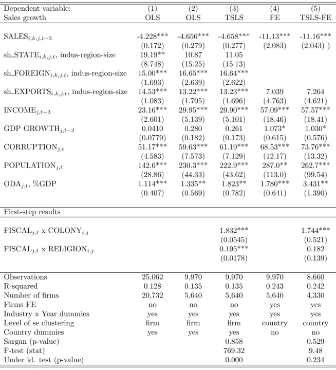
Table 3 displays the results when those three firm-level controls are replaced by their aggregation on industry-region-size. It highlights that the coefficient for foreign aid is unaltered by this change. Moreover, the effect of sh EXPORTSi,k,j,t, sh FOREIGNi,k,j,t and sh STATEi,k,j,t on firms growth is similar to the effect of EXPORTSi,k,j,t, FOREIGNi,k,j,tand STATEi,k,j,t.
Table 3: Measuring firm-level control variables on industry-region-size cells.
Dependent variable: (1) (2) (3) (4) (5)
Sales growth OLS OLS TSLS FE TSLS-FE
SALESi,k,j,t−3 -4.228*** -4.656*** -4.658*** -11.13*** -11.16***
(0.172) (0.279) (0.277) (2.083) (2.043) )
sh STATEi,k,j,t, indus-region-size 19.19** 10.87 11.05
(8.748) (15.25) (15.13)
sh FOREIGNi,k,j,t, indus-region-size 15.00*** 16.65*** 16.64***
(1.693) (2.639) (2.622)
sh EXPORTSi,k,j,t, indus-region-size 14.53*** 13.22*** 13.23*** 7.039 7.264
(1.083) (1.705) (1.696) (4.763) (4.621) INCOMEj,t−3 23.16*** 29.95*** 29.90*** 57.09*** 57.57*** (2.601) (5.139) (5.101) (18.46) (18.41) GDP GROWTHj,t−3 0.0410 0.280 0.261 1.073* 1.030* (0.0779) (0.182) (0.173) (0.615) (0.576) CORRUPTIONj,t 51.17*** 59.63*** 61.19*** 68.53*** 73.76*** (4.583) (7.573) (7.129) (12.17) (13.32) POPULATIONj,t 142.6*** 230.3*** 222.9*** 287.0** 262.7*** (28.86) (44.33) (43.62) (113.0) (99.54) ODAj,t, %GDP 1.114*** 1.335** 1.823** 1.780*** 3.431** (0.407) (0.569) (0.782) (0.641) (1.390) First-step results
FISCALj,t x COLONYi,j 1.832*** 1.744***
(0.0545) (0.521)
FISCALj,t x RELIGIONi,j 0.195*** 0.182
(0.0178) (0.139)
Observations 25,062 9,970 9,970 9,970 8,660
R-squared 0.128 0.135 0.135 0.243 0.242
Number of firms 20,732 5,640 5,640 5,640 4,330
Firms FE no no no yes yes
Industry x Year dummies yes yes yes yes yes
Level of se clustering firm firm firm country country
Country dummies yes yes yes no no
Sargan (p-value) 0.858 0.529
F-test (stat) 769.32 9.48
Under id. test (p-value) 0.000 0.234
Columns (1) and (2) are estimated using the OLS estimator, with country and industry x year dummies and robust standard errors clustered at the firm level. Columns (3) is estimated using the TSLS estimator, with country and industry x year dummies and robust standard errors clustered at the firm level. Columns (4) and (6) are estimated using the within estimator, with firms fixed-effects, industry x year dummies and robust clustered standard errors at the country level. Column (5) is estimated using the TSLS estimator with firms fixed effects, industry x year dummies and robust clustered standard errors at the country level. ***p<0.01, **p<0.05, *p<0.1.
4.2.2 Net versus Gross disbursements
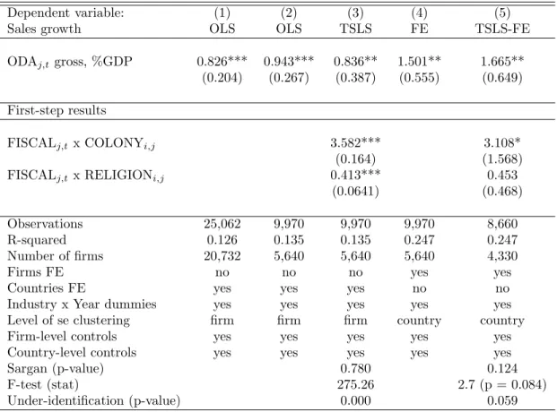
The second robustness check consists in examining the stability of the results when using aid gross disburse-ments instead of aid net disbursedisburse-ments, which are net of repaydisburse-ments. The correlation between net and gross disbursements is quite high (0.95, p-value = 0.000), and we would expect both variables to have a similar impact on firms growth. However, they do not measure the same thing: gross disbursements are a good proxy for the level of investments of donors in receiving countries while net disbursements are a good proxy for the financing capacity of the receiving countries. This robustness check is particularly important in our analysis. As discussed below, in order to understand the mechanisms through which aid flows influence firms growth, we will be looking at the impact of various sector aid variables on the constraints they face. Those sector aid variables are only available for gross disbursement and the remaining of our analysis will therefore switch from using net disbursements to using gross disbursements.
Table 4 reproduces our benchmark results with gross disbursements and underlines the stability of the results to changing the definition of aid. Column (4) of Table 4 reproduces our core estimation with gross disbursements. It suggests that a one percent increase in aid gross disbursements would lead to an increase of around 1.5 percentage point of the growth rate of enterprises in the receiving countries.
The results in Column (5) suggest that the instruments perform more poorly for gross disbursements than for net disbursements. As for net disbursements, the instrument FISCALj,t x RELIGIONi,j is not significant in the first-step, but it implies a drop in the F-test which gets to the low value of 2.7. However, when we exclude this instrument, and only keep FISCALj,t x COLONYi,j, the first-step results are better.9 The correlation of FISCALj,t x COLONYi,j with gross disbursements in the first-step is 3.935 (p-value = 0.009) and the first-step F-test is 7.94 (p-value = 0.009). The impact of aid on growth in the second-step is virtually unchanged, the coefficient being 2.064 (p-value = 0.027).
Table 4: Replacing net aid disbursements with gross aid disbursements.
Dependent variable: (1) (2) (3) (4) (5)
Sales growth OLS OLS TSLS FE TSLS-FE
ODAj,tgross, %GDP 0.826*** 0.943*** 0.836** 1.501** 1.665**
(0.204) (0.267) (0.387) (0.555) (0.649)
First-step results
FISCALj,tx COLONYi,j 3.582*** 3.108*
(0.164) (1.568)
FISCALj,tx RELIGIONi,j 0.413*** 0.453
(0.0641) (0.468)
Observations 25,062 9,970 9,970 9,970 8,660
R-squared 0.126 0.135 0.135 0.247 0.247
Number of firms 20,732 5,640 5,640 5,640 4,330
Firms FE no no no yes yes
Countries FE yes yes yes no no
Industry x Year dummies yes yes yes yes yes
Level of se clustering firm firm firm country country
Firm-level controls yes yes yes yes yes
Country-level controls yes yes yes yes yes
Sargan (p-value) 0.780 0.124
F-test (stat) 275.26 2.7 (p = 0.084)
Under-identification (p-value) 0.000 0.059
Columns (1) and (2) are estimated using the OLS estimator, with country and industry x year dummies and robust standard errors clustered at the firm level. Columns (3) is estimated using the TSLS estimator, with country and industry x year dummies and robust standard errors clustered at the firm level. Column (4) is estimated using the within estimator, with firms fixed-effects, industry x year dummies and robust clustered standard errors at the country level. Column (5) is estimated using the TSLS estimator with firms fixed effects, industry x year dummies and robust clustered standard errors at the country level. ***p<0.01, **p<0.05, *p<0.1.
4.2.3 Specification tests
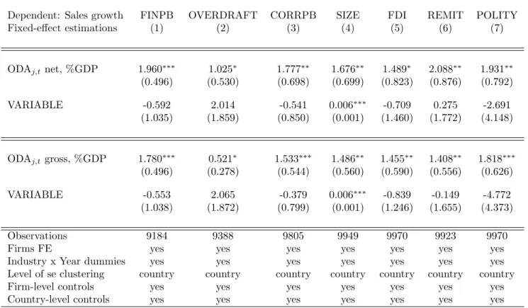
We next turn to specification tests. In Table 5 we introduce sequentially various firm-level and country-level characteristics in the benchmark regressions of Columns 4 of Tables 2 and 4. All regressions also include the same country and firm-level control variables as in the benchmark regression. In Columns (1) to (4) we introduce additional firm-level variables. The coefficient of aid - either measured in net or gross disbursements - is not altered by the introduction of FINPB (whether credit access is considered as a major obstacle), OVERDRAFT (whether the firm benefits from an overdraft facility), CORRPB (whether
corruption is considered as a major obstacle) and SIZE (number of employees).10 In Columns (5) to (7) we include additional country-level characteristics, that if correlated with aid and firms performances may induce an omitted variable bias. It turns out that neither FDI (foreign direct investment as a percentage of GDP), nor REMIT (workers remittances as a percentage of GDP), nor POLITY (the polity score provided by POLITY IV) have a significant influence on our sample of firms growth performance. The coefficient of the aid variable is unchanged when these variables are introduced in the benchmark estimations.
Table 5: Specification tests.
Dependent: Sales growth FINPB OVERDRAFT CORRPB SIZE FDI REMIT POLITY
Fixed-effect estimations (1) (2) (3) (4) (5) (6) (7) ODAj,tnet, %GDP 1.960∗∗∗ 1.025∗ 1.777∗∗ 1.676∗∗ 1.489∗ 2.088∗∗ 1.931∗∗ (0.496) (0.530) (0.698) (0.699) (0.823) (0.876) (0.792) VARIABLE -0.592 2.014 -0.541 0.006∗∗∗ -0.709 0.275 -2.691 (1.035) (1.859) (0.850) (0.001) (1.460) (1.772) (4.148) ODAj,tgross, %GDP 1.780∗∗∗ 0.521∗ 1.533∗∗∗ 1.486∗∗ 1.455∗∗ 1.408∗∗ 1.818∗∗∗ (0.496) (0.278) (0.544) (0.560) (0.590) (0.556) (0.626) VARIABLE -0.553 2.065 -0.379 0.006∗∗∗ -0.839 -0.149 -4.772 (1.038) (1.872) (0.799) (0.001) (1.246) (1.655) (4.373) Observations 9184 9388 9805 9949 9970 9923 9970
Firms FE yes yes yes yes yes yes yes
Industry x Year dummies yes yes yes yes yes yes yes
Level of se clustering country country country country country country country
Firm-level controls yes yes yes yes yes yes yes
Country-level controls yes yes yes yes yes yes yes
Estimation using the within estimator, with firms fixed-effects, industry x year dummies and robust clustered standard errors at the country level. All estimations include country and firm-level control variables. FINPB is a dummy equal to one if the firm declares access to credit to be a major obstacle to its activity. OVERDRAFT is equal to one if the firm declares having an overdraft facility. CORRPB is equal to one if corruption is a major obstacle to firm activity. SIZE is the number of employees. FDI is the ratio of foreign direct investment in GDP. REMIT is the ratio of workers remittances in GDP. POLITY is the POLITY IV indicator (-10, +10). ***p<0.01, **p<0.05, *p<0.1.
4.2.4 Sample dependence
We then explore the robustness of our results to changes in sample. Sample-dependence is an issue that is particularly acute in the aid effectiveness literature. Table 15 in Appendix 2 presents the results obtained for the fixed-effect benchmark estimation when each country is excluded one at the time. Column (1) presents the coefficient of net disbursements. Column (2) presents the coefficients of gross disbursements. Table 15 in Appendix 2 suggests that the coefficient of aid (net or gross) obtained in the fixed-effect estimations is unchanged by the exclusion of one country at the time.
As presented in Appendix 1, different numbers of firms have been surveyed in the countries of our sample. The number of observations spans from 96 (Niger) to 842 (Argentina). As our variable of interest, aid, is measured at the country level, this implies that some countries, those in which a larger number of firms was interviewed, are over-represented in our sample. In Table 6 we display the results when each country is given the same weight, by drawing randomly the same number of enterprises from each survey. In Columns (1) and (2) we draw randomly 40 firms for each country and then expend the number of firms to 70 (Columns (3) and (4)) and 100 (Columns (5) and (6)). As before, we use Columns (4) of Tables 2 and 4 as our benchmarks to run this exercise. The coefficients for aid - either measured as net or gross inflow - are very close to the coefficients of aid in Columns (4) of Tables 2 and 4.
Table 6: Random draw of firms.
Dependent: Sales growth 40 firms 70 firms 100 firms
Type of aid Net Gross Net Gross Net Gross
Fixed-effect estimations (1) (2) (3) (4) (5) (6) ODAj,t, %GDP 2.474*** 1.751*** 2.019*** 1.675*** 1.776*** 1.607*** (0.559) (0.318) (0.655) (0.445) (0.616) (0.486) Observations 2,302 2,302 3,750 3,750 4,758 4,758 R-squared 0.285 0.294 0.245 0.252 0.226 0.232 Number of Firms 1,151 1,151 1,875 1,875 2,379 2,379
Firms FE yes yes yes yes yes yes
Industry x Year dummies yes yes yes yes yes yes
Level of se clustering country country country country country country
Firm-level controls yes yes yes yes yes yes
Country-level controls yes yes yes yes yes yes
ODA is measured as a percentage of GDP, either in net flows or gross flows. Estimation using the within estimator, with firms fixed-effects, industry x year dummies and robust clustered standard errors at the country level. All estimations include country and firm-level control variables. ***p<0.01, **p<0.05, *p<0.1.
4.2.5 Attrition
World Bank Enterprise Surveys are sampled in a way as to be representative at the country level, with three levels of stratification: region, industry and size. However, the firms are representative for each round of survey; but the firms which were interviewed twice (two rounds) only represent one fourth of the total initial sample of firms. Obviously, there is no reason to believe that the firms that are interviewed twice are representative at the national level.
One related question is the issue of selection bias. If the firms that are interviewed twice are so because they are more likely to survive (better performance, specific activity, etc.) and if the probability to survive is somewhat related to how much aid is received in the country, then the estimated aid effect could be biased. There is no simple answer to this issue, as well as to the potential lack of representativeness of our sample.
In Table 7 we present simple mean-comparison tests of the growth rate of the firms, comparing those which survive in period two with those which do not. We compare the initial characteristics of these two groups, that is in period one. Table 7 suggests that the initial performance of the two groups of firms are not significantly different.
The remaining of Table 7 presents the same exercise, but comparing the firms that appear in period two to the firms that were already in the sample in period one. The growth rate of the two groups of firms seems to be significantly different, with the firms in panel displaying on average lower growth rates than the firms that appear in period 2.
Table 7: Mean-comparison tests, by period.
Group 1 Group 2
Firms which do not survive Firms which survive Difference p-value
SALES GROWTHi,k,j,t 10.14 10.92 -0.787 0.189
Observations 9074 4781
Group 1 Group 2
Firms which appear in period 2 Firms which survive Difference p-value
SALES GROWTHi,k,j,t 5.92 4.75 1.182 0.052
Observations 8018 5189
In the upper part of the table, firms of group 1 and 2 are compared for period one only. In the lower part of the table firms are compared in period 2 only.
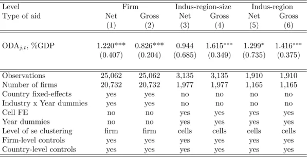
Table 7 suggests that attrition may indeed bias our results and calls for further investigation. In Table 8, we first reproduce the results obtained on the sample of all firms, using the OLS estimator. Despite the absence of firm-fixed effects, the results are similar to those obtained in the benchmark estimations.
We then turn to re-aggregating all variables on cells at the industry-region-size. All information concern-ing the 25,062 observations in the database is now used. We estimate the average growth rate computed at the industry-region-size level as a function of cells characteristics (share of firms in the cell that are state-owned, or owned by foreign investors, or exporting), as well as of the country-level characteristics. We include cells fixed effects and control for a time trend. Columns (3) and (4) present the results. Despite the fact that the coefficients are very close to those of the benchmark estimations (and not statistically different), the coefficient for net disbursements is no longer significant. The coefficient for gross disbursements remains significant at the 10% level.
Table 8: Re-aggregating at the industry-region-size and industry-region level.
Level Firm Indus-region-size Indus-region
Type of aid Net Gross Net Gross Net Gross
(1) (2) (3) (4) (5) (6)
ODAj,t, %GDP 1.220*** 0.826*** 0.944 1.615∗∗∗ 1.299∗ 1.416∗∗∗
(0.407) (0.204) (0.685) (0.349) (0.735) (0.375)
Observations 25,062 25,062 3,135 3,135 1,910 1,910
Number of firms 20,732 20,732 1,977 1,977 1,165 1,165
Country fixed-effects yes yes no no no no
Industry x Year dummies yes yes no no no no
Cell FE no no yes yes yes yes
Year dummies no no yes yes yes yes
Level of se clustering firm firm cells cells cells cells
Firm-level controls yes yes yes yes yes yes
Country-level controls yes yes yes yes yes yes
ODA is measured as a percentage of GDP, either in net flows or gross flows. In Columns (1) and (2) OLS estimations. In columns (3) to (6), estimation using the within estimator, with cells fixed-effects where cells are either industry x region x size cells or industry x region cells. All regressions include a year dummy. Robust clustered standard errors at the cells level. All estimations include country and firm-level control variables. ***p<0.01, **p<0.05, *p<0.1.
In our framework, there is a trade-off between solving the attrition bias and the endogeneity bias. The finer the level of analysis (firm or industry-region-size cells), the smaller is likely to be the endogeneity bias. However, the larger may be the selection issue. Indeed, despite the fact that the data is re-aggregated on cells, a large number of cells are only available for one period of time and do not provide information when
using the within estimator with cells fixed-effects. On the other hand, the larger is the size of the cells, the larger is likely to be the endogeneity bias. But then the attrition bias is likely to be smaller since the panel is relatively more balanced.
In Columns (5) and (6) of Table 8 we therefore use cells aggregated at the industry-region level, for which the attrition bias is likely to be smaller than in Columns (3) and (4). Overall, the results are very similar to the benchmark estimations, and confirm the positive impact of aid on firms growth.
4.3
Magnitude of the effect
Table 2 and Table 4 suggest that a one percentage point increase in aid would increase growth by 1.50-1.77 percentage point. While the magnitude of the effect seems large compared to what is usually found in the literature, it needs to be related to the level of average growth in our sample. A firm with an average annual growth rate of 7.71 (mean value of our sample, see Table 1), would see its growth rate increase by around 20-23% if aid was increased by one percentage point.
Table 9 compares the percentage increase in growth that would stem from a one percentage point increase in aid using different regressions as benchmarks. Using firm-level estimations, we report the coefficients ob-tained from the OLS and fixed-effects estimations using net disbursements (Table 2) and gross disbursements (Table 4). To compare this effect to what is usually found in the literature, we use Clemens et al. (2011) who reproduce Burnside and Dollar (2000) and Rajan and Subramanian (2008) results using extended datasets.11 They find that overall a one percentage point increase in aid would increase the income growth rate by around 0.1-0.3 percentage points in the following years.12 Because these studies look at national income per capita growth rate, the average value of growth of their sample is much lower (around 1.34-1.62 annual growth rate) than the average value of firms sales growth. For example, an economy growing at 1.34% per year would see its growth rate increased by 19.8% if aid was increased by one percentage point, and assuming that a one percentage point increase in aid increases growth by 0.265 percentage point.
Table 9 suggests that (1) the OLS estimator tends to under-estimate the impact of aid, this bias being relatively larger on aggregated data than on firms data ; (2) controlling for country fixed-effects (columns (2), (4), (6), and (8)) leads to estimates of an impact of a one percentage point increase in aid in the range of 12% to 22% of increase in average growth. Overall, the magnitude of our results appears thus to be in line with those found in the aid growth literature.
11They also lag the aid variable.
Table 9: Magnitude of the effect and comparison with other studies.
Firm’s sample Clemens et al. (2011)
Brunside and Dollar Rajan and Subramanian
Table 2 Table 4 Table 7 Table 9
Col(4) Col(5) Col(4) Col(5) Col(6) Col(7) Col(6) Col(7)
OLS WITHIN OLS WITHIN OLS FD OLS FD
(1) (2) (3) (4) (5) (6) (7) (8)
Impact of one percentage point increase in aid:
In percentage point of growth 1.346 1.770 0.943 1.501 0.117 0.265 0.070 0.187
Average growth rate 7.71 7.71 7.71 7.71 1.34 1.34 1.62 1.62
Increase in average growth (%) 17.5 22.9 12.2 19.5 8.75 19.8 4.3 11.6 The first line of Columns (5) to (8) report the estimated effect of a one percentage point increase in aid from 5.5 to 6.5 percent of GDP. Clemens et al. (2011) explain their calculation in footnote 27 page 609 of their article. The corresponding average level of growth are from Table 3 page 601 of their article.
In Columns (5) to (8) aid is lagged.
In Columns (1) and (2) net disbursements are used while in Columns (3) and (4) gross disbursements are used.
In Columns (2) and (4), WITHIN refers to the fixed-effect estimator; in Columns (6) and (8) FD refers to the estimation after first-differencing the equation.
5
Is aid enhancing the productive capacity of firms? Indirect
ev-idence of the absence of Dutch disease
The set of previous results suggest that aid tends to enhance firms growth. The literature has highlighted some mechanisms through which aid may positively affect firms performance. Foreign aid may overall increase the productive capacity of the country, either by financing basic infrastructure or investing in human capital. However, evidence on how aid may relieve the infrastructure constraints is still scarce.
If aid were to increase the productive capacity of firms, then we should expect that it does not induce, as contrarily argued by Rajan and Subramanian (2011), a decrease in the competitiveness of firms, the so-called Dutch disease. Indeed, this is the lack of absorptive capacity of aid that is at the heart of the Dutch disease mechanism: the increase in demand provoked by aid inflows is not met by an increase in supply, hence increasing prices. If aid allows firms to increase their supply, then the pressures on prices should be lower, hence attenuating Dutch disease.
So far, our results contradict those of Rajan and Subramanian (2008) who find that aid has no impact on aggregate growth. Rajan and Subramanian (2011) explain the absence of aid impact on growth by the fact that aid induces Dutch disease, i.e. a loss of competitiveness of the firms that are most likely to export.
The evidence they provide on the Dutch disease effect of aid is indirect. Building on the approach adopted by Rajan and Zingales (1998), they look at the effect of aid on industry growth rate for those industries that are more prone to export.
In what follows, we explore the Dutch disease effect of aid, or, more specifically the absence of Dutch disease. We interpret this absence of Dutch disease effect of aid as an indirect evidence that aid contributes to the adjustment of the supply side to the increase in demand, notably by increasing the productive capacity of the firms.
We follow Rajan and Subramanian (2011) and explore whether aid has a distinct impact on exporting firms. We therefore interact aid with a measure of ’exportability’ of the firms. Like them we construct various measures of ’exportability’, the most direct being a dummy for whether the firm exports its production, or part of it - EXPORTSi,k,j,t. This measure is complemented with an indicator of EXPORTABILITYi,k,j,t, which is equal to one if the firm exports more than country average.13
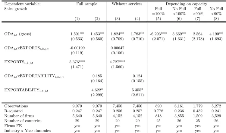
The results are presented in Table 10. Columns (1) and (2) highlight that foreign aid has a positive impact on firms growth independently of their proneness to export, measured either by EXPORTSi,k,j,t (Column (1)) or EXPORTABILITYi,k,j,t (Column (2)). This implies that the impact of aid is not different for those firms that export, indirectly suggesting the absence of Dutch disease mechanism. In Columns (3) and (4) of Table 10, we exclude from the sample the firms of the service sectors, since they are less likely to have an outward-orientation than the firms of the manufacturing sector. The results are overall consistent with the results on the full sample.
Overall, the results of the four first Columns of Table 10 provide indirect evidence for the absence of Dutch disease i.e. absence of a negative impact of aid on the outward-looking enterprises. One reason for the discrepancy between our results and those of Rajan and Subramanian (2011) may be that they aggregate their data at the industry level, while we work at the firm level. Moreover, the samples of countries are very different, which may also induce large differences in the results.
13We tested the robustness of the results to alternative definitions of ’exportability’, using EXPORTABILITY2 i,k,j,t (a
dummy variable which is equal to one if the firm exports more than the median of its industry in its country) and EXPORTABILITY3i,k,j,t (a dummy variable which is equal to one if the firm exports more than the median of all firms
Table 10: Absence of Dutch disease and firms productive capacity, indirect evidence.
Dependent variable: Full sample Without services Depending on capacity
Sales growth Full No Full Full No Full
=100% <100% >90% <90% (1) (2) (3) (4) (5) (6) (7) (8)
ODAj,t (gross) 1.501** 1.453** 1.824** 1.783** -6.293*** 3.669** 2.564 4.190**
(0.563) (0.560) (0.709) (0.710) (2.071) (1.631) (2.178) (1.693) ODAj,txEXPORTSi,k,j,t -0.00199 0.00647
(0.119) (0.106) EXPORTSi,k,j,t 5.376*** 4.727***
(1.471) (1.560)
ODAj,txEXPORTABILITYi,k,j,t 0.185 0.124
(0.164) (0.155) EXPORTABILITYi,k,j,t 4.622* 5.355* (2.299) (2.811) Observations 9,970 9,970 7,450 7,450 890 6,161 1,779 5,272 R-squared 0.247 0.247 0.256 0.257 0.778 0.236 0.432 0.241 Number of firms 5,640 5,640 4,152 4,152 818 3,855 1,509 3,529 Number of countries 29 29 29 29 25 26 25 26
Firms FE yes yes yes yes yes yes yes yes
Industry x Year dummies yes yes yes yes yes yes yes yes
Columns (1) to (8) are estimated using the within estimator, with firms fixed-effects, industry x year dummies and clustered standard errors at the country level. ***p<0.01, **p<0.05, *p<0.1.
The absence of evidence on a Dutch disease effect of aid suggests that the supply-side has managed to adjust to the increase in demand induced by aid inflows. This may notably be the case if aid contributes to increasing the productive capacity of the firms. As underlined by Guillaumont and Guillaumont Jeanneney (2007) the appreciation of the real exchange rate is likely to occur in the cases where the productive capacity is fully utilized. In cases where the productive capacity is under-utilized, the supply elasticity may be relatively high allowing for an adjustment of the supply-side, hence avoiding the loss of competitiveness (see Guillaumont and Guillaumont Jeanneney (2007), page 7).
The WBES provide information on the share of the productive capacity that is used by firms. The average percentage of utilization of the capacity is 70% for our sample of firms. It is 72% on average in Africa and in Latin America, and only 58% in the two Asian countries of the sample (Pakistan and Bangladesh).
Table 10 reports the results when we distinguish the impact of aid on growth according to whether the firm’s productive capacity is fully utilized or not. The impact of aid on growth is estimated on two separate
sub-samples: (1) the sub-sample of firms which declare using 100% of their productive capacity (Full) ; (2) the sub-sample of firms which declare using less than 100% of their productive capacity (No full). Columns (5) and (6) display the results and suggest that the positive impact of aid on growth is mainly at play for firms which are under-utilizing their productive capacity. It is significantly negative when estimated on the sample of firms which declare using 100% of their capacity, consistently with the Dutch disease hypothesis. In the last two Columns of Table 10 we test the robustness of the results to changing the threshold for under-utilization of capacity, in order to have more balanced sub-samples. We divide the sample using 90% of capacity utilization as the threshold. Lowering the threshold for full capacity induces a loss of significance of the coefficient of aid, which no longer has a significantly negative effect (even if under-utilization of capacity is only 10%, there is prospect for supply-side adjustment). The impact of aid on firms which utilize less than 90% of their capacity (Column (6)) remains significantly positive.
6
Does aid relax the constraints on growth?
In the last Section of this article, we examine the mechanisms which may explain the positive impact of aid on growth and the absence of Dutch disease. One way through which aid may increase the productive capacity of the enterprises is by relaxing the infrastructure constraints that they face. We explore this mechanism and focus on two potential infrastructure constraints: access to electricity and transports. Those two constraints may be particularly acute for manufacturing firms, those whose activity is more intensive in electricity and transports.
One way to look at whether the impact of aid on growth goes through infrastructure constraints is to include them into the baseline estimations and examine whether the impact of aid is modified. If relieving the infrastructure constraint is a channel through which aid is effective then its impact should disappear, or at least diminish.
We use the following three aggregate variables for infrastructure from the World Development Indicators (2013):
• ELECTRICITYj,t: Electric power consumption, kwh per capita, in logarithm. • RAILj,t: km of railways, in logarithm.
• ROADj,t: Km of paved roads, in percentage of total area.
Those infrastructure variables have a lot of missing values, implying the loss of many observations. For example, introducing RAILj,tinto the estimation induces the loss of 10 countries and an overall loss of 3,156 observations. The same applies to all four infrastructure variables, at various degrees. Because we want to look at how the coefficient of aid evolves when the infrastructure variables are added to the baseline model, we first reproduce the baseline estimation on the restricted samples corresponding to each infrastructure variables. The results are presented in Panel A of Table 11.
Despite the change in sample, the impact of aid on firms growth remains significantly positive. Its magnitude is substantially modified by the fact that it is estimated on smaller samples - it even reaches 10,16 % in Column (2) when estimated on the (very restricted) sample of RAILj,t.
Panel B of Table 11 presents the results when the infrastructure variables are introduced into the baseline estimations, and ODAj,tis dropped. We find that both proxies for electricity and railways infrastructure are positive and significantly correlated with firms growth. The proxy for road infrastructure is not significant and negative. Data on roads have become poorer recently and it is therefore possible to have a better panel of countries when lagging this variable by one period. The results when LAGGED ROADj,tis substituted for ROADj,t are presented in Column (4) of Table 11. Of course, if we want to compare the impact of aid with and without LAGGED ROADj,t, contemporary aid is not relevant and the right variable to use is LAGGED ODAj,t. Column (4) suggests that the density of paved road is significantly and positively correlated with firms performances in the following period. 14
Finally, Panel C of Table 11 presents the results when ODAj,t and the infrastructure variables are introduced simultaneously. Overall, the impact of aid remains significant, but the magnitude of the impact is reduced. In Column (1), introducing ELECTRICITYj,tinto the baseline estimation induces a drop in the coefficient of ODAj,t from 2.63 to 2.42. In Column (2) the coefficient of ODAj,t drops from 10.15 to 7.93. Finally, in Column (4), the coefficient of LAGGED ODAj,t is reduced from 1.99 to 1.72. The coefficient of LAGGED ROADj,tis now only borderline significant (p-value = 0.115).
14The fact that LAGGED ROAD
j,t is significant, while ROADj,t is not is mainly due to the change in sample. When
Table 11: Infrastructure as a channel of the aid impact on firms growth using country-level variables
Dependent variable: Sales growth (1) (2) (3) (4)
INFRASTRUCTURE: ELECTRICITY RAIL ROAD LAGGED ROAD
Panel A
ODAj,t gross disb., % GDP 2.634∗∗∗ 10.155∗∗ 1.588∗ 2.215∗∗∗
(0.869) (4.437) (0.843) (0.781)
Lagged ODAj,t−1 gross disb., % GDP 1.999∗∗
(0.756)
Panel B
INFRASTRUCTUREj,t 52.053∗∗ 171.550∗∗∗ -1.512 8.543∗∗
(25.143) (57.646) (2.972) (3.828)
Panel C
ODAj,t gross disb., % GDP 2.415∗∗∗ 7.930∗∗∗ 1.684∗ 1.468∗∗
(0.796) (2.340) (0.900) (0.716)
INFRASTRUCTUREj,t 47.186∗ 130.485∗∗∗ -2.330 6.783
(23.084) (36.027) (2.727) (4.172)
LAGGED ODAj,t−1 gross disb., % GDP 1.719∗∗
(0.720)
Observations 9220 6814 8657 9529
Number of firms 5212 4120 5368 5577
Number of countries 24 19 28 29
Firms FE yes yes yes yes
Industry x Year dummies yes yes yes yes
Level of se clustering country country country country
Firm-level controls yes yes yes yes
Country-level controls yes yes yes yes
Columns (1) to (4) are estimated using the within estimator, with firms fixed-effects, industry x year dummies and clustered standard errors at the country level. INFRASTRUCTUREj,t is either ELECTRICITY (Column (1)), RAIL
(Column (2)), ROAD (Column (3)), or LAGGED ROAD (Column (4)). ***p<0.01, **p<0.05, *p<0.1.
Overall, the results of Table 11 suggest that the level of development of infrastructure is spurring firms growth in developing countries. The results are also consistent with the idea that part of aid’s impact on sales growth is channeled through infrastructure.
We now turn to looking more directly at the impact of aid on firms infrastructure constraints. We proceed in two steps. First, we look at how the infrastructure constraints, measured at the firm level, influence their
growth performance and the probability that the enterprise is under-utilizing its productive capacity. Second, we look at the impact of aid on those constraints.
6.1
Impact of infrastructure obstacles on firms growth and capacity
The WBES provide an assessment of the obstacles faced by firms. Indeed, the respondents are asked the kind of problem they face in their activity. Some of those assessments are more objective than others. For example, whether or not the firm had to face power outages is obviously more objective than the perception by the manager of the electricity problems faced by his firm. Those perception variables are also more prone to endogeneity issues since the firms with lower performance may be likely to have a rougher assessment of the infrastructure constraints. We therefore use various measures to provide a picture as broad as possible of the different constraints weighing on firms growth. We use the following firm-level variables to proxy the infrastructure obstacles faced by firms:
• ELECTRICITY di,k,j,t: dummy variable which is equal to one if the firm considers electricity as a major or severe obstacle.
• POWERi,k,j,t: dummy variable which is equal to one if the firm had to face power outages during the fiscal year.
• TRANSPORT di,k,j,t: dummy variable which is equal to one if the firm considers transport as a major or severe obstacle.
• TRANSPORT mi,k,j,t: dummy variable which is equal to one if the firm considers transport as its main obstacle.
Despite the fact that they are all supposed to measure the infrastructure obstacles to firms activity, those four variables tend to be weakly correlated one with the others. For example, ELECTRICITY di,k,j,t and POWERi,k,j,thave a correlation of 0.21 (p-value = 0.000). The correlation is even weaker (0.098, p-value = 0.000) for TRANSPORT di,k,j,t and TRANSPORT mi,k,j,t. The perception variables of the infrastructure obstacles are those which are the most correlated: ELECTRICITY di,k,j,tand TRANSPORT di,k,j,thave a correlation of 0.26 (p-value = 0.000).
Panel A of Table 12 presents the effect of each of the constraints, introduced sequentially, on both sales growth and capacity under-utilization. When looking at the impact of the firm-level infrastructure obstacles on growth and under-capacity we exclude aid from the regressions. Indeed, infrastructure obstacles and aid
are correlated which blurs the results when looking at the impact of any of these variables on growth.15 In columns (1) to (4), where the outcome is sales growth, we can see that not all the variables capturing the constraints at the firm-level have a significant effect on growth. However, both electricity and transport infrastructure seem to matter for firms growth. Electricity problems, captured by POWERi,k,j,t, significantly decrease the growth rate. Transport obstacles, as measured by TRANSPORT mi,k,j,t, also significantly decrease the growth rate of firms.
Not all the firms have answered to the questions on the obstacles to their activity. Depending on the variable used to capture the constraints, we therefore loose some observations. To check whether the results are not driven by this reduction in sample, we therefore replace the missing observations by zero and create a dummy which is equal to one when the missing point was replaced. The results are displayed in Panel B of Table 12. They are not changed by this procedure, except for TRANSPORT mi,k,j,twhich looses significance (p-value = 0.129).
In Columns (5) to (8) of Table 12, we explore the impact of the infrastructure obstacles measured at the firm-level on whether firms under-utilize their capacity. Indeed, if we assume that aid increases the productive capacity of firms by relaxing the constraints they face, then it is important to check that those constraints do indeed imply a lower productive capacity. The dependent variable in columns (5) to (8) -UNDER-CAPACITY di,k,j,t - is a dummy variable which is equal to one whenever the capacity utilization is lower than 100%. We therefore switch from the within estimator to the probit estimator. In the probit estimations, along the firm-level and country-level control variables16, we also control for country dummies, industries x year dummies, and cluster the standard errors at the firm-level. Panel A of Table 12 suggests that, again both electricity (captured by POWERi,k,j,t) and transport (captured by TRANSPORT di,k,j,t) obstacles increase the probability that the firm will be under-utilizing its productive capacity. The results are confirmed in Panel B, when the missing observations are replaced by zero, suggesting that they are not driven by the reduction in sample due to missing observations for obstacles.
15The correlation of gross disbursements with POWER
i,k,j,tis 0.194***. It is 0.074*** with ELECTRICITY di,k,j,t, 0.059***
with TRANSPORT mi,k,j,tand 0.019*** with TRANSPORT di,k,j,t.
16The control variables introduced in the probit estimations are the same as those introduced in the OLS estimations of Table
Table 12: Impact of infrastructure constraints on firms growth and capacity
Dependent variable: GROWTH (fixed-effect estimations) UNDER-CAPACITY (probit estimations) (1) (2) (3) (4) (5) (6) (7) (8) Panel A POWERi,k,j,t -2.311∗∗ 0.095∗∗ (1.041) (0.046) ELECTRICITY di,k,j,t 0.219 0.037 (1.028) (0.044) TRANSPORT mi,k,j,t -11.785∗ -0.191 (5.796) (0.170) TRANSPORT di,k,j,t 1.585 0.077∗ (1.016) (0.043) Observations 9630 9940 8151 9876 6828 7034 5296 7017 Number of firms 5617 5632 5497 5623 4040 4051 3896 4050 Number of countries 29 29 29 29 26 26 26 26 Panel B POWERi,k,j,t -2.293∗∗ 0.079∗ (1.032) (0.044)
Missing POWERi,k,j,t 3.465 -0.313∗∗
(7.038) (0.132)
ELECTRICITY di,k,j,t 0.166 -0.006
(1.035) (0.043)
Missing ELEC di,k,j,t 7.188 -0.386
(7.763) (0.344)
TRANSPORT mi,k,j,t -8.960 -0.182
(5.732) p=0.13 (0.166) Missing TRANS mi,k,j,t 17.063∗∗ 0.233∗∗∗
(7.779) (0.086)
TRANSPORT di,k,j,t 1.362 0.110∗∗∗
(1.027) (0.042)
Missing TRANS di,k,j,t -17.063 0.151
(11.972) (0.278)
Observations 9970 9970 9970 9970 7051 7051 7051 7051 Number of firms 5640 5640 5640 5640 4054 4054 4054 4054 Number of countries 29 29 29 29 26 26 26 26
Firms FE yes yes yes yes no no no no
Country dummies no no no no yes yes yes yes Industry x Year dummies yes yes yes yes yes yes yes yes Clustering of st. errors country country country country firm firm firm firm Firm-level controls yes yes yes yes yes yes yes yes Country-level controls yes yes yes yes yes yes yes yes
Columns (1) to (4) are estimated using the within estimator, with firms fixed-effects, industry x year dummies and clustered standard errors at the country level. Columns (5) to (8) are estimated using the probit estimator, with country and industry x year dummies and clustered at the firm level. ***p<0.01, **p<0.05, *p<0.1.