Properties of the interstellar medium of the star-forming galaxy, IC10, at various spatial scales

(1)

HAL Id: tel-01735178

https://tel.archives-ouvertes.fr/tel-01735178

Submitted on 15 Mar 2018

HAL is a multi-disciplinary open access archive for the deposit and dissemination of sci-entific research documents, whether they are pub-lished or not. The documents may come from

L’archive ouverte pluridisciplinaire HAL, est destinée au dépôt et à la diffusion de documents scientifiques de niveau recherche, publiés ou non, émanant des établissements d’enseignement et de

galaxy, IC10, at various spatial scales

Fiorella Lucia Polles

To cite this version:

Fiorella Lucia Polles. Properties of the interstellar medium of the star-forming galaxy, IC10, at various spatial scales. Cosmology and Extra-Galactic Astrophysics [astro-ph.CO]. Université Paris-Saclay, 2017. English. �NNT : 2017SACLS276�. �tel-01735178�

(2)

NNT : 2017SACLS276

Thèse de doctorat

de l’Université Paris-Saclay

préparée au Université Paris-Sud

Ecole doctorale n 127

Astronomie et astrophysique d’Île-de-France

Spécialité de doctorat : Astronomie et astrophysique

par

Mme Polles Fiorella Lucia

Properties of the interstellar medium of the star-forming galaxy,

IC 10, at various spatial scales

Thèse présentée et soutenue à Gif-sur-Yvette, le 29 september 2017. Composition du Jury :

M. Verstraete Laurent Professeur (Président du jury)

Université Paris-Sud XI/IAS

Mme Satyapal Shobita Professeur (Rapporteur)

George Mason University

M. Schilke Peter Professeur (Rapporteur)

University of Koeln

Mme Meixner Margaret Professeur (Examinatrice)

Space Telescope Science Institute

Mme Habart Emilie Maître de Conférence (Examinatrice) Université Paris-Sud XI/IAS

Mme Hughes Annie Astronome adjoint (Examinatrice)

(3)

(4)

Abstract

The InterStellar Medium (ISM) provides the details of the environment and processes that lead to star formation, which in turn, drives the evolution of a galaxy. Moreover, it is the site of stellar birth and the repository of stellar ejecta, hosting the signatures of metal enrichment. How stars have been formed in galaxies in the early universe, when heavy elements are deficient, is a fundamental issue in astrophysics. While it is hard to analyze the ISM chemistry at high redshifts, the Local Group of galaxies offers the opportunity to study several ‘chemically-young’ dwarf galaxies in detail. These dwarfs are perfect laboratories to investigate how the metal-poor ISM affects the interplay between gas, dust and stars.

This thesis project investigates the properties of the multi-phase ISM of the nearby dwarf galaxy IC10, which has a metallicity of 1/3 solar. In particular, it focuses on the analysis of the physical properties of the compact HII regions and the diffuse ionized gas, traced by the mid- and far-infrared

cooling lines. The proximity of this galaxy (d=700 kpc) enables the analysis of the ISM on different spatial scales: from the compact, bright clumps (≥25 pc) to the whole star-forming body of the galaxy (≥650pc). It has been observed with the space telescopes Spitzer and Herschel, providing a set of ≥16 infrared emission lines. I complemented this dataset with new observations made with the SOFIA airborne telescope.

I have studied the spatial distribution of the far-infrared (FIR) lines (lin-ear resolution ≥40 pc). I found that [OIII] 88µm is the brightest infrared cooling line everywhere along the body of the galaxy, suggesting a high filling factor of diffuse ionized gas. The ISM is very porous, allowing UV photons to leak from the HIIregions and traverse large distances, unique to low

metallic-ity galaxies with low dust abundance. [CII] 157.7 µm, which can arise from both ionized and neutral gas, is the second brightest FIR cooling line. De-spite the prominent ionized gas phase, the ratio [CII] 157.7 µm/[NII] 121.9 µm shows that most of the [CII] 157.7 µm emission (at least 98%) comes from the neutral Photo-Dissociation Regions (PDRs), not from the ionized gas.

(5)

lines were compared to photoionization and photodissociation models. Using

Cloudy

(Ferland et al. 2013), I have built grids of models adapted to the specific case of IC 10 and I have tested two different strategies to compare the observations with the model predictions: line ratios and absolute flux values. Since the sensitivity and the spatial coverage of the observations were not homogeneous, it was not possible to select the same combinations of tracers at the different scales. Hence, exploring those methods was necessary to extract the best possible constraints on the physical properties. The investigation suggested that, based on the dataset, the best choice was to compare all of the available tracers at each scale using the line absolute values.

The modeling enabled me to determine the properties of the brightest clumps within the galaxy and demonstrate that the emission at large scales (≥300 pc) is dominated by that of the compact, bright clumps that lie in the region. Moreover, at those large scales we found that a simple description of a single component model was not sufficient to reproduce all of the tracers. A second ionized gas component, with lower density, filling the ISM between the compact HII regions, is required.

In order to draw a complete resolved picture of the ISM composition in metal-poor galaxies, it is important to extend the analysis to the PDR/molecular phase. The next step following the PhD work is the application of the mod-elling method refined in this project to the PDR phase including the tracers [OI] 63.2 µm, [OI] 145.5 µm, [CII] 157.7 µm, CO lines as well as the total infrared luminosity (LT IR).

(6)

Résumé

Le milieu interstellaire (MIS), composé de gaz et de poussière, renferme les informations essentielles sur l’environnement et les processus menant à la for-mation d’étoiles qui, à son tour, influe sur l’évolution d’une galaxie. C’est le lieu où les étoiles naissent et déposent de la matière, dont les métaux ou élé-ments lourds. La structure du MIS n’est pas homogène; au contraire, le MIS contient plusieurs composantes avec des compositions chimiques, densités, températures, etc. différentes. L’élément en phase gazeuse le plus abondant étant l’hydrogène, une façon simplifiée de décrire les composantes du MIS est basée sur l’état d’ionisation de l’hydrogène : la phase atomique ionisée, où l’hydrogène est sous la forme ionisée notée H+_{, la phase atomique neutre,}

où l’hydrogène est sous la forme neutre notée H0_{/HI, et la phase moléculaire,}

où l’hydrogène est sous la forme de molécule de dihydrogène notée H2.

Une des questions fondamentales en astrophysique actuellement est de comprendre comment les étoiles se sont formées dans les galaxies et notam-ment dans l’univers jeune où les métaux, importants pour le refroidissenotam-ment, sont absents. S’il est difficile d’accéder à la chimie du MIS à grand redshift, le Groupe Local offre la possibilité d’étudier en détails plusieurs galaxies peu évoluées chimiquement. Ces galaxies naines sont de parfaits laboratoires pour voir comment le contenu en métaux (ou métallicité) du MIS affecte l’interaction entre le gaz, la poussière et les étoiles. Dans ce sens, le pro-gramme Herschel le Dwarf Galaxy Survey (DGS ; Madden et al. 2013) a ouvert une nouvelle porte pour l’étude des propriétés physiques du MIS dans ces galaxies. L’analyse du MIS des galaxies du DGS, à échelle intégrée donc sans résoudre spatialement les différentes phases du MIS, a mis en avance l’importance de la phase diffuse ionisée et la faiblesse de l’émission de CO (Cormier et al. 2015). Comme la molécule H2 ne peut pas être observée

directement car elle est symétrique et monucléaire, ce sont les raies de ro-tation du monoxyde de carbone, CO, qui sont généralement utilisées pour tracer le réservoir de gaz moléculaire. Et c’est à partir de ce réservoir que se forment les nouvelles étoiles. La faible émission de CO dans les galaxies à faible métallicité (Leroy et al. 2009;Schruba et al. 2012;Cormier et al. 2014)

(7)

par le fait que le MIS à faible métallicité contient des photons ionisants très énergétiques qui peuvent pénétrer plus profondément à l’intérieur des nuages atomiques et moléculaires quand la poussière est moins abondante. Ainsi ces photons peuvent dissocier les molécules comme CO plus facilement alors que la molécule de H2, qui est beaucoup plus abondante, est moins affectée car

elle peut s’auto-écrantè plus efficacement. La phase de gaz correspondant aux régions où CO est photo-dissocié et H2 est auto-écranté s’appelle le gaz

‘sombre en CO’. L’existence de cette composante de gaz sombre en CO a été suggérée d’abord à travers des observations de la raie de [CII] 157.7 µm dans le LMC par Poglitsch et al. (1995) et dans IC 10 par Madden et al. (1997). Son existence a aussi été confirmée dans la Voie Lactée (ex: Grenier et al. 2005; Planck Collaboration et al. 2011). Voir Chapitre 1.

Mon projet de thèse porte sur les propriétés du MIS multi-phases de la galaxie naine IC 10, dont la métallicité est 1/3 solaire (Chapitre 1). La proximité de cette galaxie (d=700 kpc) offre la possibilité d’analyser le MIS à plusieurs échelles spatiales: des nuages brillants compacts (25 pc) au corps entier de la galaxie formant des étoiles (650 pc). En particulier, je me suis intéressée à l’analyse des propriétés physiques des régions HIIcompactes et du

gaz ionisé diffus, que l’on trace avec les raies de refroidissement en infrarouge moyen (MIR) et lointain (FIR). Les raies de structure fine en MIR et FIR sont des traceurs puissants des propriétés du MIS ainsi que de l’activité de formation stellaire, et elles sont moins affectées par l’extinction par la poussière que les raies en optiques. Cela est important dans le cas de IC 10 car cette galaxie se situe très près du plan Galactique (b=-3.3¶). IC 10 a

été observée avec les télescopes spatiaux Spitzer et Herschel, fournissant un jeu d’environ 16 raies d’émission en infrarouge. J’ai complété ce jeu avec des observations que j’ai effectuées grâce au télescope aéroporté SOFIA (Chapitre 2).

Au Chapitre 3, je présente l’étude de la distribution spatiale des raies FIR, dont la résolution est d’environ 40 parsecs. J’ai trouvé que [OIII] 88.4 µm est la raie de refroidissement FIR la plus brillante, et ce, tout du long du corps de la galaxie, suggérant un facteur de remplissage du gaz diffus ionisé élevé. Le MIS de IC 10 semble être très poreux, ce qui permet aux photons UV de s’échapper des régions HII denses et de parcourir des distances importantes,

une caractéristique unique aux galaxies avec un contenu faible en métaux et en poussière. La raie de [CII] 157.7 µm dont l’émission peut provenir à la fois des phases ionisées et neutres, est la seconde raie FIR la plus brillante. Malgré une phase diffuse ionisée importante, le rapport de [CII] 157.7 µm/[NII] 121.9 µm indique que la plupart de l’émission de [CII] 157.7 µm (au moins 98%)

(8)

µm, révèle que la densité du gaz ionisé est d’environ 500 cm≠3.

L’émission des raies de refroidissement est fonction des conditions physiques des phases du MIS. Afin d’estimer les propriétés physiques des phases prin-cipales (densités, extinction, etc.) et la nature des sources de rayonnement ionisant, j’ai confronté les observations des raies MIR et FIR à des modèles de photoionisation et photodissociation. Pour cela, j’ai utilisé le code de synthèse spectrale

Cloudy

(Ferland et al. 2013) et construit des grilles de modèles adaptées au cas de IC 10 (Chapitre 4). Afin de produire un spec-tre observé, le code considère un nuage de gaz et de poussière à géométrie plan-parallèle et divise ce nuage en plusieurs zones en fonction de la pro-fondeur du nuage. Ensuite, le champ de radiation à l’entrée du nuage est propagé à travers ces zones et, à chaque étape, les processus physiques tels que le transfert radiatif, les réactions chimiques, les niveaux de population, etc. sont traités. Contrairement à d’autres codes,

Cloudy

permet un cal-cul cohérent de la structure thermique et chimique du gaz à travers la région HII et la PDR.

Cloudy

est donc un outil idéal pour extraire les

informa-tions physiques des nombreux traceurs infrarouge observés qui proviennent de plusieurs phases du MIS. Dans l’étude de IC 10, l’histoire de formation d’étoiles des amas stellaires responsables de l’ionisation du gaz est représentée par une flambée d’étoiles unique. Cette hypothèse est peut-être valable pour une région HIIindividuelle mais le gaz distribué à plus grande échelle spatiale

est probablement chauffé et ionisé par des populations stellaires d’âges variés. Un scenario avec un taux de formation stellaire continu pourrait être envis-agé, mais la pente du continu spectral UV en-deçà de 103 _{Å (énergies plus}

de 13.6 eV) est quasiment indépendante de l’âge de la population stellaire, ce qui rend ce scenario difficile à tester avec seulement des traceurs du gaz ionisé en main. Une étude de suivi, modélisant à la fois les raies du gaz ionisé et les raies du gaz neutre et sondant ainsi une gamme d’énergies plus large, permettra peut-être de tester ce scenario de formation d’étoiles continue.

Un des objectifs majeurs de mon projet est de comparer les conditions physiques du gaz ionisé obtenues à partir des traceurs observés aux différentes échelles spatiales étudiées. Pour cela, j’ai choisi trois échelles spatiales:

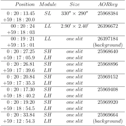
1. les “clumps”, la plus petite échelle spatiale réalisable avec la résolution des instruments. La meilleure résolution possible avec les observations de Spitzer/IRS SL est de 4”, ce qui correspond à 14 pc à la distance de IC 10. Avec cette résolution, je peux séparer les nuages brillants compacts d’une composante d’émission plus diffuse. Bien que plusieurs clumps pourraient être étudiés, je me suis restreinte à ceux qui sont les

(9)

centrale et deux dans le premier arc.

2. les “zones”, de grandes régions dans la galaxie (aire de quelques kpc2₎

dans lesquels on s’attend à ce que les conditions physiques locales soient différentes d’une région à l’autre. Certaines zones incluent des clumps et des structures visibles en H– alors que d’autres zones sont choisies pour examiner le milieu diffus ionisé.

3. le “body”, la plus grande échelle correspondant à la majeure partie du corps de la galaxie avec une activité de formation d’étoiles notable. D’une taille de 608 pc ◊ 855 pc, cette échelle inclus la plupart des zones étudiées individuellement.

J’ai développé et testé deux méthodes différentes de comparaison des obser-vations aux prédictions des modèles : l’une basée sur des rapport de raies, l’autre sur les valeurs absolues des flux des raies (Chapitre 5). Comme la sensibilité et la couverture spatiale des observations de IC 10 ne sont pas ho-mogènes, il est impossible de sélectionner et modéliser la même combinaison de raies pour toutes les échelles spatiales. Ainsi, l’exploration de ces méth-odes a été nécessaire pour établir les meilleures contraintes possibles sur les conditions physiques des régions de IC 10. Les deux méthodes diffèrent prin-cipalement dans la façon d’explorer l’espace de paramètres des modèles. La méthode de rapport des raies permet de combiner des raies provenant d’un même instrument ou d’un même élément, minimisant ainsi certaines incer-titudes. Cependant, le choix des raies à combiner pour créer les rapports a un impact sur les résultats et sur les meilleurs modèles trouvés. En effet, j’ai montré qu’en choisissant un ensemble de rapports différent, les valeurs des paramètres reproduisant au mieux ces rapports et donc les meilleurs mod-èles peuvent changer. A l’inverse, la méthode des flux des raies considère les raies telles qu’elles et ne nécessite aucune combinaison de raies. Les résultats de cette étude suggèrent que, avec le jeu de données en main, la méthode la plus performante pour comparer tous les traceurs disponibles à chaque échelle spatiale est celle utilisant les valeurs absolues des flux. Cette méth-ode suggère toutefois le besoin d’une seconde composante dans les modèles, une phase diffuse ionisée, pour mieux reproduire certaines raies observées telles que [OIII] 88.4 µm.

Mon travail de modélisation a permis de déterminer les propriétés des nuages les plus brillants dans cette galaxie ainsi que les propriétés de ré-gions plus grandes (300 parsecs), et j’ai démontré que l’émission à grande échelle spatiale est dominée par celle des clumps (Chapitre 6). Les propriétés

(10)

les régions HIIanalysées ici pourrait être reliée à la rétroaction des vents

stel-laires et supernovae dus à la génération d’étoiles précédente. Pour chaque clump, l’extinction peut être calculée, d’une part, en comparant le flux H– observé avec celui prédit par les meilleurs modèles, et d’autre part, de façon théorique avec le rapport de Hu–(7-6)/H–(3-2). Je trouve que ces deux méthodes donnent des valeurs d’extinction similaires. Un résultat important concernant les clumps est qu’ils semblent être délimités par la matière, c.-à-d. qu’il n’y a pas assez de matière pour absorber tous les photons ionisants et la taille de la région HII est définie par la taille du nuage de matière.

Ainsi, les clumps sont quasiment transparents au champ de radiation, ce qui permet à une fraction importante des photons ionisants de s’échapper de la région HII. A plus grandes échelles, le gaz devient de plus en plus délimité

par la radiation et non par la matière, c.-à-d. les régions sont optiquement épaisses au champ de radiation, ce à quoi on s’attend car les photons ion-isants s’échappant des régions HII ont plus de chance d’être absorbés au fur

et à mesure que le volume de gaz augmente. Ce scenario de photons ionisant qui s’échappent et l’échelle spatiale typique qu’ils traversent avant d’être absorbés est très intéressant dans le contexte d’un MIS poreux à faible mé-tallicité. De plus, à grande échelle, je trouve qu’aucun modèle n’arrive, seul, à reproduire l’émission de tous les traceurs de manière satisfaisante. En effet, une deuxième composante de gaz ionisé est nécessaire, avec une plus faible densité et remplissant le MIS entre les régions HIIcompactes. Cependant, le

nombre de contraintes observationnelles n’est pas suffisant pour construire un modèle fiable du MIS avec plusieurs composantes. Enfin, je me suis in-téressée à l’origine de l’émission des raies de [CII] 157.7 µm, [FeII] 25.9 µm et [SiII] 34.8 µm pour déterminer quelle fraction de leur émission provient du gaz ionisé (et non du gaz neutre). En comparant l’émission prédite par les meilleurs modèles aux observations, j’ai trouvé que la plupart de l’émission de ces raies de [CII], [FeII] et [SiII] provient de la PDR.

Pour finir, le Chapitre 7 présente les perspectives offertes par mon travail de thèse. Cette étude de modélisation de IC 10 suggère que, pour toutes les échelles spatiales étudiées, le gaz ionisé contient probablement plusieurs composantes aux caractéristiques différentes (ex : densités). L’ajout d’une autre composante dans les modèles est possible mais requiert davantage d’observables. Une possibilité serait d’inclure les raies optiques comme con-traintes additionnelles. Par exemple, le rapport des raies optiques [SII] 6716Å / [SII] 6731Å est généralement un bon traceur de la densité du gaz au front d’ionisation des régions HII. Des spectres optiques ont été obtenus pour un

(11)

Spec-problèmes d’extinction, la spectroscopie optique fournit une résolution spa-tiale supérieure à celle de la spectroscopie infrarouge, et permettra peut-être une modélisation plus détaillée de la structure du MIS. Une autre perspec-tive intéressante est le James Webb Space Telescope, une mission de la NASA dont le lancement est prévu pour fin 2018. En particulier, l’instrument en infrarouge moyen MIRI couvre les longueurs d’ondes de 4.9 µm à 28.8µm. MIRI va permettre d’observer les mêmes raies spectrales que l’IRS ainsi que des raies dont l’émission est plus faible grâce à sa sensibilité accrue, à une meilleure résolution spatiale et spectrale, ce qui sera suffisant pour séparer les diverses composantes du gaz ionisé. Cependant, avec le champ de vue restreint de MIRI (3.9” ◊ 7.7”), on ne pourra pas faire de grande carte de IC 10 et seules des petites régions HII bien ciblées pourront être observées

dans IC 10 et dans les galaxies proches.

Etendre l’analyse du gaz ionisé à la phase neutre atomique et au gaz moléculaire est important pour établir une vue complète du MIS résolu dans les galaxies à faible métallicité. La prochaine étape suivant ce travail de thèse sera donc d’appliquer la méthode de modélisation que j’ai développée à la phase PDR en incluant les traceurs: [OI] 63.2 µm, [OI] 145.5 µm, [CII] 157.7 µm, CO lines ainsi que LT IR. Un de mes objectifs est d’utiliser les modèles PDR pour estimer spatialement la masse de gaz moléculaire sombre en CO dans cet environnement à faible métallicité. Parmi les paramètres les plus importants à prendre en compte pour cela sont le rapport de gaz-sur-poussière et l’extinction des nuages.

Certains de mes résultats, comme la délimitation des régions par la matière ou par la radiation ou encore l’importance de la phase ionisée, reflètent des changements notables dans la balance des phases et dans le transport de ra-diation à faible métallicité; et cela peut avoir de fortes implications pour le refroidissement et l’évolution des galaxies dans l’univers jeune. De plus, une des perspectives principales les plus captivantes pour l’évolution des galaxies est de mieux comprendre comment les processus qui agissent aux échelles locales, comme la formation stellaire, dépendent des processus qui agissent à plus grandes échelles voire à l’échelle d’une galaxie entière, comme le MIS ou la dynamique globale d’une galaxie. Dans ce cadre, étendre mon analyse multi-échelles des propriétés du MIS (densités, champs de radiation, masses, facteurs de remplissage, etc.) à des galaxies recouvrant une gamme étendue de conditions va permettre de mieux relier les petites et les grandes échelles et de fournir des diagnostics directs sur les propriétés physiques en fonction de l’environnement galactique.

(12)

List of Figures

1.1 Schematic view of the interplay between the components of a galaxy. . . 25

1.2 Phases of the ISM. . . 27

1.3 Schematic of the photoelectric heating on the neutral gas.. . . 29

1.4 Intensity ratios of the infrared lines tracing the density. . . 32

1.5 Excitation potential versus critical density diagram. . . 33

1.6 Theoretical ratios of [NII]122/205µm, [CII]/[NII]205µm and [CII]/[NII]122µm as a function of the density for a tempera-ture of 9000 K. (Figure from Bernard-Salas et al. 2012).. . . . 36

1.7 Example of standard extinction curve. . . 38

1.8 Infrared spectrum of the Orion nebula. . . 39

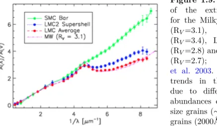
1.9 A comparison of the extinction curves for the Milky Way. . . . 40

1.10 SED fitting of three regions of IC 10: dense region in red, diffuse region in blue and intermediate region in green. The points are WISE, Spitzer and Herschel observations (Lianou et al, in prep). . . 41

1.11 Illustration of ISM phases at different metallicity. . . 45

1.12 Metallicity distribution for the DGS sample. . . 47

1.13 Histogram of the Herschel and Spitzer and other ancillary data available for the DGS sources. . . 48

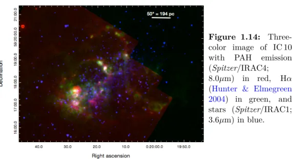
1.14 Three-color image of IC 10 with the clump position overlaid. . 50

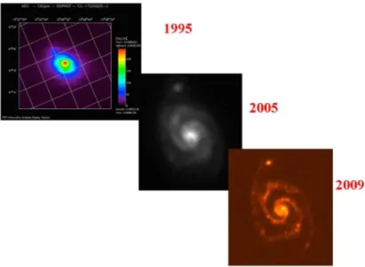
2.1 Images of M51 at 160 µm obtained by ISO, Spitzer and Herschel. 56

2.2 Spitzer configuration. . . . 58

2.3 The four IRS modules. . . 60

2.4 Schematic view of the slits and peak-up apertures. . . 60

2.5 Projection of the configuration of the slits for SL and LL ob-servations of IC 10. . . 62

2.6 Position of the HR pointing. . . 63

2.7 The Herschel spacecraft. . . . 67

2.8 Spectrometer (Left) and photometer (Right) side layout of the SPIRE focal plane unit. . . 67

(17)

2.11 Filter transmissions of the three photometric band of PACS. . 71

2.12 PACS spectrometer point-source line sensitivity as a function of wavelength and PACS spectrometer PSF as a function of wavelength. . . 72

2.13 Example of how a scan map is performed by PACS photometer. 72 2.14 PACS: Raster projection of the [CII] 157.7 µm observations IC 10 into subgrid of 3” pixels. . . 74

2.15 SOFIA Observatory. . . 75

2.16 Integral-field spectrometer of FIFI-LS. . . 77

2.17 SOFIA FIFI-LS pointings positions. . . 78

3.1 H– map (Gil de Paz et al. 2003). Red borders show the ar-eas covered by Herschel/PACS [OIII] 88.4 µm map, magenta Spitzer/IRS Short-Low maps and blue Spitzer/IRS Long-Low maps. . . 81

3.2 Spitzer/IRS SL maps. . . . 82

3.3 Spitzer/IRS LL maps. . . . 83

3.4 Herschel/PACS maps. . . . 85

3.5 H– map of IC 10 (Hunter & Elmegreen 2004). . . . 86

3.6 LF IR map of IC 10. . . 87

3.7 Observed [OIII] 88.4 µm/[CII] 157.7 µm ratio. . . . 89

3.8 Density map inferred from the observed [SIII] 33.5 µm/[SIII] 18.7 µmratio. . . . 90

3.9 Observed [CII] 157.7 µm[NII] 121.9 µmratio. . . . 92

3.10 Comparison of theoretical and observational [NII] 121.9 µm /[CII] 157.7 µm . . . . 92

3.11 Observed [OI] 63.2 µm/[CII] 157.7 µm ratio. . . . 93

4.1 Schematic view of the configuration of ionized code. . . 100

4.2 Schematic view on modeling technique. . . 101

4.3 Scheme of the multi-phase ISM structure modeled by Cloudy. 102 4.4 Stellar population spectra for a single burst. Left - Spectra for fixed total mass at different ages. Right - Spectra for a fixed age at different stellar masses. . . 105

4.5 Stellar population spectra for continuous star formation. Left: Spectra for a fixed SFR of at different ages. Right: Spectra for fixed age at different SFR. . . 106

4.6 Open geometry and spherical geometry in

Cloudy

. . . 109

(18)

the H– background image. The Body zone corresponds to the largest area that we investigated. . . 121

5.3 The Spitzer/IRS and Herschel/PACS lines for the Central

main zone. . . . 121

5.4 Example of the decomposition obtained with the Rxy method. 123

5.5 Comparison of the Spitzer line fluxes determined for the three clumps in the Central main zone. . . . 125

5.6 Comparison of the PACS line fluxes determined for the three clumps in the Central main zone. . . . 126

5.7 Comparison of the Spitzer line fluxes determined for the two clumps in the ArcA region. . . . 127

5.8 Comparison of the PACS line fluxes determined for the two clumps in the ArcA region. . . . 128

5.9 PDFs for nH, log U, tburst, and physical depth for the Central

main zone with the line ratio method, set number 1. . . . 134

5.10 PDFs for the Central main zone with the line ratio method, set number 2. . . 135

5.11 Left: The observed line ratios (solid lines) are plotted in the model parameter space log U vs. log nH. Right: ‰2

distribu-tion in the parameter space. . . 137

5.12 PDFs for the clump Center c1 with the line ratio method. . . 139

5.15 PDFs for the clump ArcA c1 with the line ratio method. . . . 142

5.16 PDFs for the clump ArcA c2 with the line ratio method. . . . 143

5.17 Histograms of the distribution of the parameters for the clumps

Center c1, Center c2 and Center c3 with the line ratio method.145

5.18 Histograms of the distribution of the parameters for the clumps

ArcA c1 and ArcA c2 with the line ratio method. . . . 146

5.19 Results for the Central main zone with the line ratio method. 150

5.20 Results for the ArcA zone with the line ratio method. . . . 152

5.21 Results for the ArcB zone with the line ratio method. . . . 153

5.22 Results for the Intermediate zone with the line ratio method. 154

5.23 Results for the Central north zone with the line ratio method. 155

5.24 Results for the West zone with the line ratio method. . . . 156

5.25 Results for the Diffuse zone with the line ratio method. . . . . 157

5.26 Results for the Body zone with the line ratio method. . . . 158

5.27 PDFs for the clump Center c1 with the absolute line flux method. . . 163

(19)

5.30 PDFs for the clump Center c2 with the absolute line flux method, including [SIII] 33.5 µm/[SIII] 18.7 µm as constraint. 166

5.32 PDFs for the clump Center c3 with the absolute line flux method, including [SIII] 33.5 µm/[SIII] 18.7 µm as constraint. 168

5.33 PDFs for the clump ArcA c1 with the absolute line flux method.169

5.34 PDFs for the clump ArcA c1 with the absolute line flux method, including [SIII] 33.5 µm/[SIII] 18.7 µm lines as constraint. . . 170

5.35 PDFs for the clump ArcA c2 with the absolute line flux method.171

5.36 PDFs for the clump ArcA c2 with the absolute line flux method, including [SIII] 33.5 µm/[SIII] 18.7 µm lines as constraint. . . 172

5.37 Histograms of parameter distributions for the best models for the clumps Center c1, Center c2, and Center c3 with the ab-solute line flux method.. . . 174

5.38 Histograms of parameter distributions for the best models for the clumps ArcA c1 and ArcA c2 with the absolute line flux method. . . 175

5.39 PDFs for the clumps Center c1, Center c2 and Center c3 with the absolute line flux method. The PDF overplotted in red is for the subset of the models with tburst between 2.8-3.3 Myr. . 176

5.40 PDFs for the clumps ArcA c1 and ArcA c2 with the absolute line flux method. The PDF overplotted in red is for the subset of the models with tburst between 2.8-3.3 Myr. . . 177

5.41 PDFs for the clumps Center c1, Center c2 and Center c3 from top to bottom. The PDF overplotted in red is for the subset of the models with tburst between 5.2-5.8 Myr. . . 178

5.42 PDFs for the clumps ArcA c1 and ArcA c2 from top to bottom. The PDF overplotted in red is for the subset of the models with tburst between 5.2-5.8 Myr. . . 179

5.43 PDFs of observed vs. predicted constraint values for the clump

Center c1. . . 181

Center c2. . . 182

5.45 PDFs of observed vs. predicted constraint values for clump

(20)

ArcA c2. . . 185

5.48 Results for the Central main zone with the absolute line flux method. . . 187

5.49 Results for the ArcA zone with the absolute line flux method. 188

5.50 Results for the ArcB zone with the absolute line flux method. 189

5.51 Results for the Intermediate zone with the absolute line flux method. . . 190

5.52 Results for the Central north zone with the absolute line flux method. . . 191

5.53 Results for the West zone with the absolute line flux method . 192

5.54 Results for the Diffuse zone with the absolute line flux method.193

5.55 Results for the Body zone with the absolute line flux method. 194

5.56 PDFs of the observed vs. predicted constraint values for the

Central main zone. . . . 196

6.1 Examples of extinction curves used for the Milky Way. . . 205

6.2 PDFs of the observed over predicted [SiII] 34.8 µm and [CII] 157.7 µm for the zones Central main zone , ArcA and ArcB.. 211

6.3 PDFs of the observed over predicted [SiII] 34.8 µm (left) and [FeII]25 µm (right), for the North zone. See Figure 6.2 for the plot description. . . 212

6.4 PDFs of the observed over predicted [SiII] 34.8 µm for the zones Intermediate , Diffuse and Body. . . . 213

7.1 Density diagnostic plots using the [OIII] ratio. . . 223

7.2 SOFIA/FIFI-LS Cycle 5 preliminary maps of the FIR fine structure line [OIII] 51.8µm in Central main zone (left) and

ArcA zone (right) in units of [Jy]. . . . 224

7.3 Multi-component modeling of the Central main zone. . . . 225

7.4 Gas temperature and line emission across a standard cloud with Cloudy.. . . 226

(21)

(22)

List of Tables

1.1 Characteristics of the ISM phases in the Galaxy . . . 30

1.2 Properties of the infrared fine-structure cooling lines. . . 31

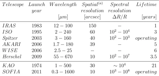
2.1 List of infrared and submillimetre telescopes. . . 57

2.2 Main properties of the IRS modules. . . 61

2.3 Summary of IRS observations of IC 10. . . 64

2.4 Fluxes obtained with HR modules for each pointing used in this work. . . 66

2.5 SPIRE spectrometer characteristics. . . 68

2.6 SPIRE photometer characteristics. . . 69

2.7 General capabilities of the instruments onboard SOFIA (from SOFIA Observer’s Manual). . . 76

4.1 Elemental abundances used to model the HII regions of IC 10

with

Cloudy

. . . 111

5.1 Integrated fluxes for each zone . . . 120

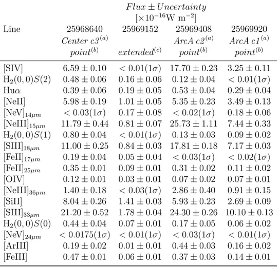
5.2 Fluxes (◊1e-16 W m≠2 ) for each clump using the different

decomposition methods. . . 124

5.3 Results of the best model parameters with 1‡ uncertainties for each clump for the line ratio method. . . 144

5.4 Results for each zone using the line ratio method. . . 160

5.5 Results of the best model parameters with 1‡ uncertainties, obtained with the absolute flux method.. . . 183

5.6 Summary of the results for each zone. . . 197

6.1 Comparison of the extinction E(B-V) determined toward the clumps in IC 10. . . 206

6.2 E(B-V) from previous works. . . 206

6.3 Integrated fluxes of [CII]157.7µm, [FeII] 25.9µm and [SiII] 34.8

(23)

(24)

Chapter 1 The Interstellar Medium of

Dwarf Galaxies

1.1 Galaxy

The word galaxy is derived from the Greek galaxias (“–⁄–›í–Î), literally “milky”, a reference to the Milky Way. Until well into the twentieth century, it was by no means clear that any object existed beyond the confines of the Milky Way. In the mid-eighteenth century Immanuel Kant published his treatise, General Natural History and Theory of the Heavens, in which he suggested that the Milky Way might not be the only stellar system, and that some of the nebulae (faint, fuzzy, approximately elliptical patches of light seen in the sky) might be complete island universes, similar in structure to the Milky Way but viewed from large distances and at a variety of angles to the line of sight. Towards the end of the eighteenth century, increasingly powerful telescopes led to more systematic studies of nebulae. In 1922, Edwin Hubble observed Cepheid variable stars in the Andromeda Nebula and estimated their luminosities. Measuring their apparent brightness then yielded a direct estimate of their distances. Using this method, Hubble obtained a value for the distance to Andromeda of some 300 kpc. So it firmly demonstrated that the Andromeda Nebula was not an element within the Milky Way, but it was a comparable stellar system in its own right.

A galaxy is a gravitationally-bound collection of stars, stellar remnants, an interstellar medium (ISM) of gas and dust, surrounded by a dark mat-ter halo with each component emitting at a different wavelength. In the band between the ultraviolet (UV) and near-infrared (NIR), the radiation is mainly due to an ensemble of stars, with spectra resembling black bodies having emission peaks at different wavelengths, depending on the temper-ature. Young stars (few Myr) peak in the UV at ≥ 0.1 µm, while older stars (0.1 - 1 Gyr) peak in the visible at ≥0.5 µm. At longer wavelengths, thermal emission from warmer dust is observed (hundreds of K) in the mid-infrared (MIR), to colder dust (tens of K) in the far-mid-infrared (FIR). At radio wavelengths, synchrotron emission from relativistic particles, accelerated by supernovae explosions and thermal free-free emission from ionized plasma, can be observed. The distribution of the total energy emitted by a galaxy at various wavelengths is the spectral energy distribution (SED). The emission from gas, unlike that of stars and dust, is not contributing to the continuum emission of the SED, but through spectral line emission and absorption over the whole electromagnetic spectrum.

The repartition of these different components can vary from galaxy to galaxy, influencing the evolution and the properties we observe. In the Milky Way, for example, the total baryonic mass is dominated by the stellar mass, while the ISM (dust and gas) represents only 2.5% (Tielens 2005). The luminosity of the ISM, however, contributes to 30% of the total luminosity

(26)

of the Milky Way.

All of the galaxy components are interrelated and participate in the evo-lution of the galaxy, which is due to the cyclic process between stars and the ISM. The low mass stars, through their stellar winds, eject dust and metals produced by the stellar nucleosynthesis, to the surrounding medium. The more massive stars explode in supernovae at the end of their lives, enriching the ISM with metals. The gas and dust of the ISM, now more metal rich, is then recycled, forming clouds that collapse gravitationally to form stars. A schematic view of this continuous interplay between the star, gas and dust components, is shown in Figure 1.1.

Figure 1.1: Schematic view of the interplay between the components of a galaxy. The visible components of a galaxy are the stars, the gas and the dust. All of those components are related: at the end of their lives, massive stars explode in supernovae, releasing metal elements into the surrounded medium. The gas and dust, thus enriched, then collapse to form a new generation of stars.

Hence, the ISM is a fundamental component of a galaxy. It is the birth-place of stars, and on the other hand its properties, structure, composi-tion and chemical evolucomposi-tion are driven by feedback processes, such as stellar winds, supernovae, emission of ionizing photons, etc. In order to trace a galaxy’s evolution, it is thus fundamental to understand the processes that link the ISM to the stars and how the properties of the dust and gas affect

(27)

the star formation activity of galaxies.

1.2 Phases of the Interstellar Medium

This work is focused on the investigation of the gas components of the ISM, which represent around 99% of the ISM. Most of the gas is hydro-gen (≥71.8%), followed by helium (≥27%), the rest consists of gaseous met-als. The ISM gas structure is not homogeneous; on the contrary it shows a multi-component structure of different compositions, densities, tempera-tures, abundances, etc. A rather simplified way to view the ISM, since the dominant element of the gas is hydrogen, is to consider the ISM based on the ionization state of hydrogen: ionized atomic phase, where the hydrogen is in the H+_{, neutral atomic phase, where the hydrogen is in the neutral}

atomic form, H, and molecular phase, where hydrogen is in the molecular form, H2. Typical physical properties of the different gas phases are

summa-rized in Table 1.1 and shown in schematic form in Figure 1.2. More details on the chemistry and physics of the ISM can be found in Tielens(2005) and

Osterbrock & Ferland(2005).

1.2.1 Ionized phase

Photons with energies greater than 13.6 eV, produced by hot stars, ionize the surrounding gas creating HII regions. These are normally young stars

(Æ15 Myr), typically O and B stars, which link the HII regions to the recent

star formation. Therefore, HII regions are often studied to determine the

present day chemical abundances (Yin et al. 2010;López-Sánchez et al. 2011;

Garnett 1990). The compact HII regions around the ionizing sources are

typically characterized by densities of ≥ 105 _cm≠3 while the more diffuse

ionized regions are on the order of ≥ 1 cm≠3. Temperatures of H_II regions

can be ≥ 102 _{to 10}4 _{K. Their linear scales can be a few parsecs, such as the}

Orion nebula (D≥8 pc) to hundreds of parsecs, such as NGC5471 (D≥1 kpc;

García-Benito et al. 2011).

Ionizing photons escaping from HII regions, ionize the diffuse ISM,

creat-ing the Warm Ionized Medium (WIM). This component is characterized by very low densities (10≠1 cm3) and can have one of the largest filling factors

in galaxies.

The primary heating source of the ionized phases is photoionization. Ion-ized species collide with electrons in the gas and fine structure lines are emit-ted via radiative decay from UV to IR wavelengths. Highly ionized species, such as S3+ _{and Ne}2+_{, probe the dense H}_II _{regions in close proximity to the}

(28)

Figure 1.2: Schematic of the phases of the ISM of galaxies. Bottom: A global picture of the complex ISM phases of a galaxy showing ionized regions and neutral atomic and molecular cloud complexes embedded within a more diffuse phase, which can be neutral in part and mostly ionized. Top: A zoom into the layered interfaces of the ionized, neutral and molecular phases (Figure fromCormier 2012). UV photons produced by the stars ionize the surrounding gas creating a HII region.

Photons with energy less than 13.6 eV (ionization potential of H0_{) escape from}

the HII region and penetrate deeper into the cloud, creating the photodissociation

region, where the hydrogen is neutral, CO is photodissociated and carbon is ionized (ionization potential of C0 _{is 11.3 eV). Finally, deeper into the cloud, the gas is}

in molecular form. Each of these phases can be traced by various emission lines (Section 1.2.4).

exciting stars since they require the most energetic photons, while species with lower ionization states, such as N+ _{and Ne}2+ _{originate in the more}

extended, diffuse ionized gas.

The Hot Ionized Medium (HIM) is characterized by extreme temperatures (≥105 _{- 10}6 _{K) and very diffuse gas (≥ 3◊10}≠3 cm≠3), carrying a small mass

fraction of the ISM. This phase is ionized normally by shocks generated by supernovae explosions and stellar winds and emits thermal X-ray continuum and highly-excited emission lines, such as N4+_{, O}6+ _{and O}7+_.

(29)

1.2.2 Neutral atomic phase

Much of the ISM of galaxies is composed of neutral atomic hydrogen, par-ticularly in disk galaxies. The atomic phase is identified by the dominance of atomic H in the interface phase where the UV photons have energy less than 13.6 eV, but where H2 molecules do not exist. This phase, consisting of

neutral atomic species such as H0_{, C}0 _{and O}0_{, is most easily traced by the}

21 cm HI line.

The neutral phase can be divided in two very different components: the Cold Neutral Medium (CNM) and the Warm Neutral Medium (WNM). The CNM is a cool, diffuse HI cloud with typical temperatures of ≥100 K and densities of ≥50 cm≠3. The WNM is an intercloud gas at temperatures

typically of ≥8000 K and densities of ≥0.5 cm≠3.

The neutral interface between the HII region and the molecular core is

the PhotoDissociation Region (PDR; Figure1.2). The physics and chemistry of this transition phase is controlled by FUV photons which have escaped the HII region with 6 < h‹ <13.6 eV. These photons ionize species with

ioniza-tion potentials less than 13.6 eV, such as C, Si and S and dissociate molecular hydrogen. Deeper into the cloud the ionizing photons are sufficiently attenu-ated allowing H2 to exist, forming the dense, molecular core. In dense PDRs

this transition between the PDR and the molecular phase occurs near visual extinction, AV (see section 1.2.5), ≥2 magnitudes.

The heating of this phase is primarily via two processes: the photoelectric effect and FUV pumping of H2. The photoelectric effect occurs when a FUV

photon is absorbed by a dust grain and an energetic electron is ejected into the gas, transferring energy to heating the gas. This process is illustrated in Figure 1.3. The efficiency of the photoelectric heating depends on the size and the charge of the grains. The efficiency increases inversely with grain size. Hence the most efficient dust components are the smallest grains, the polycyclic aromatic hydrocarbons (PAHs) and other small grains. The charge of the grains is given by the balance between the photoionization and the electron recombination, which is controlled by “ = G0T1/2/ne, where

G0 is the radiation field (Tielens & Hollenbach 1985) and ne is the electron density. The second source of heating in the PDRs is the FUV pumping of H2. The molecule H2 absorbs photons via the Lyman-Werner electronic

transitions ( E > 11.2 and 12.3 eV). Most of the time the H2 cascades to

an excited vibrational level in the ground electronic state via fluorescence while 10 to 15% of the FUV pumping events, the molecule will dissociate via fluorescence to the ground electronic state.

The cooling of the PDR gas is due mainly to IR fine-structure line emis-sion from species such as [CII] 157.7 µm , [OI] 63.2 µm and [OI] 145.5 µm .

(30)

Figure 1.3: Schematic of the photoelectric heat-ing via the dust grains and PAHs (Figure from Tielens 2005). The efficiency, ‘, is a function of fn for PAH and of Y for the grains. fnis the probability of the PAH to be ionized by the FUV pho-tons, while Y is the prob-ability that the electron es-capes from the grain.

1.2.3 Molecular phase

The molecular phase is the densest component of the ISM and exists where H2 dominates the gas phase. While H2 is the most abundant molecule, other

molecules are forming within this phase, shielded from dissociating photons, such as CO, HCN, O2. The molecular phase is characterized by densities >

102 _cm≠3 and temperatures on the order of ≥10 K.

Molecules can form on the surface of dust grains and can be destroyed by UV photons if their self-shielding efficiency or the shielding from the dust is insufficient. For example, for H2 the Lyman-Werner bands become optically

thick at high density; hence the molecule can be shielded from starlight. On the other hand, CO, which is the second most abundant molecule, is not as efficiently self-shielded, but relies on the dust to shield it from the dissociating photons.

FUV photons and cosmic rays are the main heating sources of molec-ular clouds. Molecules, excited by collisions and shocks, cool the gas via vibrational and rotational transitions emitted in the FIR to submillimeter (submm) wavelength range. A prominent coolant in the molecular gas phase is CO in its various rotational transitions.

1.2.4 Observational tracers

The state of the ionized, PDR, and molecular phases can be derived by studying the emission lines, which emit at various wavelengths. Baldwin et al.(1981), for example, proposed the [OIII]⁄5007/H— and [NII]⁄6584/H– diagnostic diagram (the BPT diagram) to separate the line-emission objects based on the excitation mechanism: HII regions, planetary nebulae, and

(31)

Table 1.1: Typical characteristics of the ISM phases in the Galaxy and principal ways to observe the phases. Table adapted from Tielens(2005)

Phase T [K] n [cm≠_3] _M(a)_[109_M

§] Observation

Hot Ionized Medium 105 _{- 10}6 _0.003 _- _{Thermal X-ray emission}

Ionized metal absorption/emission lines Thermal radio emission

HII regions 104 _{1 - 10}5 _0.05 _{Thermal radio emission}

H– recombination line FIR fine-structure lines Bright MIR continuum Warm Ionized Medium 8000 0.1 1.0 H– recombination line

Thermal radio emission

Warm Neutral Medium 8000 0.5 2.8 HI 21 cm absorption/emission line Cold Neutral Medium 80 50 2.2 HI 21 cm emission line

Molecular cloud 10 > 200 1.3 CO rotational lines (a) Representative mass of the phases in the Milky Way.

simple line ratios can sometimes characterize the physical properties of the emitted gas. For example, the ratio of lines of the same element but different ionization stage, such as [NeIII] 15.5 µm /[NeII] 12.8 µm , traces the tem-perature of the ionizing source, while the ratio of lines of the same ion but different transition, can estimate the electron density (Osterbrock & Ferland 2005;Abel et al. 2005). Consider two levels with the same excitation energy but with different Einstein A coefficients (rate of spontaneous emission and absorption) or collisional de-excitation rates, the excitation of these levels will be related only by different densities. Examples of ratios that can be used to measure the gas electron density are [SII]6716/[SII]6731 Å in the optical and [OIII]88/[OIII]52 µm in the IR. Figure1.4 shows examples of in-frared line ratios that trace different density regimes. Each line ratio, in fact, can trace the density of the gas when the value of the density lies between the critical densities of the two lines. The critical density is the density for which the collisional rate coefficient is equal to the radiative de-excitation co-efficient. For densities higher that this threshold density, collisions dominate the de-excitation process.

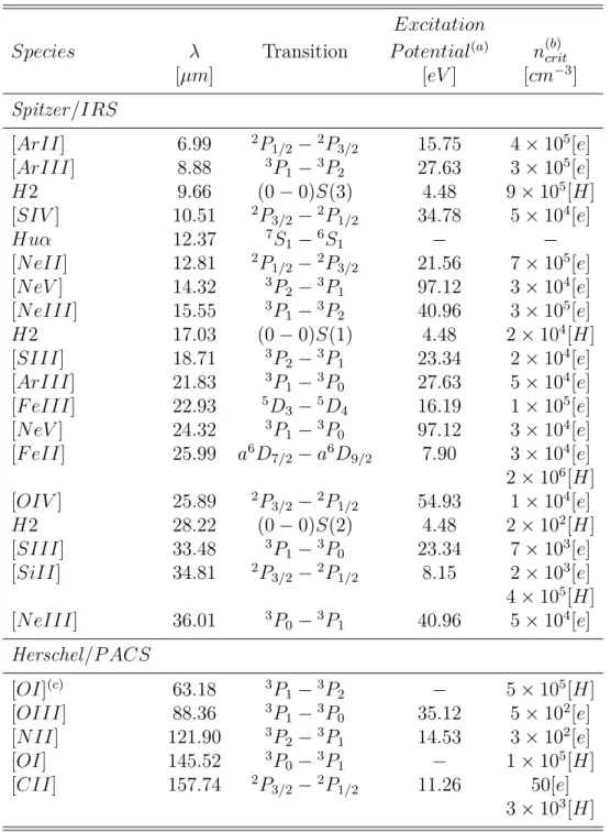
Unlike the optical lines, infrared observations are slightly effected by ex-tinction (see Section1.2.5) and they cover a wide range of excitation poten-tials and critical densities (Figure 1.5; Kennicutt et al. 2011). The wave-lengths, excitation potentials and critical densities of the MIR and FIR lines observed with Spitzer and Herschel space telescopes (see Chapter2), are pre-sented in Table 1.2.

(32)

Table 1.2: Properties of the infrared fine-structure cooling lines observed with

Spitzer and Herschel space telescopes.

Excitation

Species ⁄ Transition P otential(a) n(b)crit

[µm] [eV ] [cm≠3] Spitzer/IRS [ArII] 6.99 2_P 1/2≠2P3/2 15.75 4 ◊ 105[e] [ArIII] 8.88 3_P 1≠3P2 27.63 3 ◊ 105[e] H2 9.66 (0 ≠ 0)S(3) 4.48 9 ◊ 105[H] [SIV ] 10.51 2_P 3/2≠2P1/2 34.78 5 ◊ 104[e] Hu– 12.37 7S1≠6S1 ≠ ≠ [NeII] 12.81 2_P 1/2≠2P3/2 21.56 7 ◊ 105[e] [NeV ] 14.32 3_P 2≠3P1 97.12 3 ◊ 104[e] [NeIII] 15.55 3_P 1≠3P2 40.96 3 ◊ 105[e] H2 17.03 (0 ≠ 0)S(1) 4.48 2 ◊ 104[H] [SIII] 18.71 3_P 2≠3P1 23.34 2 ◊ 104[e] [ArIII] 21.83 3_P 1≠3P0 27.63 5 ◊ 104[e] [F eIII] 22.93 5_D 3≠5D4 16.19 1 ◊ 105[e] [NeV ] 24.32 3_P 1≠3P0 97.12 3 ◊ 104[e] [F eII] 25.99 a6_D 7/2≠ a6D9/2 7.90 3 ◊ 104[e] 2 ◊ 106_[H] [OIV ] 25.89 2_P 3/2≠2P1/2 54.93 1 ◊ 104[e] H2 28.22 (0 ≠ 0)S(2) 4.48 2 ◊ 102[H] [SIII] 33.48 3_P 1≠3P0 23.34 7 ◊ 103[e] [SiII] 34.81 2_P 3/2≠2P1/2 8.15 2 ◊ 103[e] 4 ◊ 105_[H] [NeIII] 36.01 3_P 0≠3P1 40.96 5 ◊ 104[e] Herschel/P ACS [OI](c) _63.18 3_P 1≠3P2 ≠ 5 ◊ 105[H] [OIII] 88.36 3_P 1≠3P0 35.12 5 ◊ 102[e] [NII] 121.90 3_P 2≠3P1 14.53 3 ◊ 102[e] [OI] 145.52 3_P 0≠3P1 ≠ 1 ◊ 105[H] [CII] 157.74 2_P 3/2≠2P1/2 11.26 50[e] 3 ◊ 103_[H]

(a) Energy required to create the ion. (b) Critical density for collisions with electrons [e] or with hydrogen atoms [H].

(33)

Figure 1.4: Intensity ratios of the infrared lines of [OIII], [SIII], [NeIII] and [ArIII] as a function of the electron density. (Figure from

Tielens 2005).

MIR fine-structure lines

The MIR fine-structure lines, observed by Spitzer, are diagnostics mostly of the compact ionized gas (Spinoglio et al. 2015;Abel et al. 2005), due to their high critical density and excitation potential. In the following I present the MIR tracers that I have used in my PhD study.

• [ArII] 6.9 µm and [ArIII] 8.9 µm

Ar0 _{and Ar}+ _{have ionization potentials of 15.7 and 27.6 eV,}

respec-tively, and critical densities for collisions with electrons of 4 ◊ 105

cm≠3 for [ArII] 6.9 µm and 3 ◊ 105 cm≠3 for [ArIII] 8.9 µm . Since

these two lines are emitted by two different ionization stages of the same element, the ratio [ArIII] 8.9 µm /[ArII] 6.9 µm traces the hard-ness of the radiation field. [ArIII] 8.9 µm , requiring the higher energy to ionize, would originate closer to the radiation source in the dense HII regions than [ArII] 6.9 µm , which would be emitted more from the

outer shell of the HII regions. Therefore, the ratio [ArIII] 8.9 µm /[ArII]

6.9 µm can trace the leakage of ionizing photons from the HII regions

(Section 4.3.2).

• [NeII] 12.8 µm and [NeIII] 15.5 µm

Of the two MIR neon lines, the [NeIII] 15.5 µm has a much higher excitation potential, requiring 41 eV photons to ionize the Ne+ _while

(34)

Figure 1.5: Excitation potential versus critical density for the fine-structure cooling lines observed with Spitzer and Herschel space telescopes. (Adapted from

Kennicutt et al. 2011).

Ne0_{, requires 21.6 eV to create Ne}+ _(Table _1.2_{). The [NeII] 12.8 µm}

and [NeIII] 15.5 µm are exclusively found in HII regions. The critical

density of [NeII] 12.8 µm for collisions with electrons is 7 ◊ 105 _cm≠3,

while for [NeIII] 15.5 µm the critical density with electrons is lower, 3 ◊ 105 cm≠3. However, while [NeIII] 15.5 µm is associated only with

dense, hot HII regions, [NeII] 12.8 µm can arise from HII regions as well

as relatively diffuse low-ionization gas (Cormier et al. 2012; Dimaratos et al. 2015). Since these two lines are emitted by different ionization stages of the same element, the ratio [NeIII] 15.5 µm/[NeII] 12.8 µm traces the hardness of the radiation field.

(35)

• [SIII] 18.7 µm , [SIII] 33.5 µm and [SIV] 10.5 µm

S+ _{has an ionization potential of 23.3 eV and traces the ionized gas.}

The two [SIII] transitions at 18.7 µm and 33.5 µm have critical den-sities with electrons of 2 ◊ 104 _cm≠3 and 7 ◊ 103 cm≠3, respectively.

Hence the ratio [SIII] 33.5 µm/[SIII] 18.7 µm is a useful density tracer. S2+_{, has an ionization potential of 34.7 eV and [SIV] has a critical}

density for collisions with electrons of 5 ◊ 104 _cm≠3, tracing the dense

hot HII regions. The combination of [SIV] 10.5 µm with [SIII] 18.7

µm , as well as [SIII] 33.5 µm , provides useful ratios to measure the hardness of the radiation field.

• [FeII] 25.9 µm and [SiII] 34.8 µm

Fe+ _{and Si}+ _{ions require ionizing photons lower than that of}

hydro-gen (7.9 eV to ionize Fe0 _{and 8.2 eV to ionize Si}0_{; see Figure} _1.5_).

Therefore, Fe+ _{and Si}+ _{may exist in the neutral gas, excited mostly by}

H0_{, H}

2 and free electrons, as well as in the ionized gas, excited by

elec-trons. In order to understand which phase these lines trace, modeling of the full suite of lines is required.

FIR fine-structure lines

The FIR fine-structure lines are important diagnostics of the properties of the ionized phase as well as of the PDR phase (Wolfire et al. 1990; Kaufman et al. 2006). They have been observed in the past with ISO and the KAO, in more recent past with Herschel and now with SOFIA.

• [OIII] 88.4 µm

[OIII] 88.4 µm has an excitation potential of 35.1 eV and a critical density 500 cm≠3, thus arises only from ionized gas. The combination

of [OIII] 88.4 µm with [OIII] 52 µm, is a useful constraint of electron density the HII region (Lebouteiller et al. 2012). [OIII] 52 µm was not

accessible with Herschel, but can now be observed with SOFIA (Sec-tion 2.4.3).

• [CII] 157.7 µm

[CII] 157.7 µm is one of the most important cooling lines of the ISM. It has been studied in many different environments, including Galactic

(36)

PDRs (Bennett et al. 1994), dwarf galaxies (e.g. Madden et al. 1997;

Cormier et al. 2015; Fahrion et al. 2016), spiral galaxies (e.g. Kapala et al. 2017), high-redshift galaxies (Neeleman et al. 2017). Usually it is the brightest FIR emission line in galaxies, which can sometimes be used to determine the redshift of galaxies (e.g. Brada et al. 2017) and its luminosity can be used as a measure of the star formation rate in galaxies (e.g. De Looze et al. 2011).

The ionization potential of C0 _{is 11.3 eV, less than that of hydrogen}

(13.6 eV). Thus C+_{, in principle, may exist in the ionized phase, excited}

by collisions with electrons with a critical density of 50 cm≠3, as well

as in the neutral phase, excited by H or H2 with a critical density of

2.8◊103_cm≠3. The potential for [CII] 157.7 µm to exist in different

phases complicates the interpretation of this popular diagnostic. In our Galaxy, [CII] 157.7 µm has been found to trace the surface layers of PDRs. For example,Bernard-Salas et al. (2012) have found that in the Orion Bar > 82% of the [CII] emission is coming from the PDR region. Similar conclusions have been determined for [CII] 157.7 µm observed around the 30Doradus region in the Large Magellanic Cloud (Chevance et al. 2016). However [CII] 157.7 µm has also been observed to originate in the ionized gas phase (Madden et al. 1993; Abel et al. 2005; Cormier et al. 2012).

There are several methods to disentangle the origin of [CII] 157.7 µm. It can be done through detailed modeling (e.g. Bernard-Salas et al. 2012; Cormier et al. 2012) or by inspecting key diagnostic line ratios, such as [CII] 157.7 µm/[NII] 121.9 µm as explained below (e.g. Oberst et al. 2011).

• [NII] 121.9 µm and [NII] 205.2 µm

N+_{with an excitation potential of 14.5 eV originates only in the ionized}

phase. The two FIR transitions, [NII] 121.9 µm and [NII] 205.2 µm, with relatively low critical densities of 300 cm≠3 and 45 cm≠3,

respec-tively, when used as a ratio, become a useful electron density tracer of the diffuse ionized gas, as is shown in Figure 1.6. Since these lines can only arise from the ionized phase while the origin of [CII] 157.7 µm is ambiguous, the ratios [NII] 121.9 µm/[CII] 157.7 µm and [NII] 205.2 µm/[CII] 157.7 µm can be used to disentangle the origin of [CII] 157.7 µm . In particular, since [CII] 157.7 µm and [NII] 205.2 µm have very similar critical densities and excitation temperatures, the ratio of

(37)

[CII]/[NII] depends mostly on the abundances of N+ _{and C}+ ₍_Oberst

et al. 2006;Oberst et al. 2011; Bernard-Salas et al. 2012).

Figure 1.6: Theoretical ratios of [NII]122/205µm, [CII]/[NII]205µm and [CII]/[NII]122µm as a function of the density for a temperature of 9000 K. (Figure from

Bernard-Salas et al. 2012).

• [OI] 63.2 µm and [OI] 145.5 µm

The two [OI] lines at 63.2 and 145.5 µm, together with [CII] 157.7 µm , are the dominant coolants in PDRs. These two lines have critical densities of 5◊105 _{and 10}5 _cm≠3, respectively and excitation energies

of 228 and 325 K. The ratio [OI] 145.5 µm /[OI] 63.2 µm is a popular diagnostic used to determine the physical conditions in PDRs ( Kauf-man et al. 1999). In particular, this ratio can be used to estimate the density and temperature of the neutral gas: the ratio increases with increasing temperature and decreases with decreasing density (Tielens & Hollenbach 1985). The [OI] 63.2 µm is one of the brightest cool-ing lines (Oberst et al. 2011; Bernard-Salas et al. 2012; Cormier et al. 2015) but is known to be affected by optical depth effects (Tielens & Hollenbach 1985; Abel et al. 2007; Chevance et al. 2016). The [OI] 145.5 µm line, however, is fainter than the 63.2 µm line, often by at least an order of magnitude, making it a challenge, even for Herschel, to map large regions in galaxies.

(38)

Molecular lines

• H2

H2 is the most abundance molecule in galaxies. However, it is a

sym-metric molecule and does not have a permanent dipole moment, making this molecule difficult to observe. Nevertheless, its rotational quadrupole transitions ( J = ±2; defining J as the rotational quantum number) have been observed in the MIR with Spitzer. These lines (3.4 to 28µm) are pure rotational transitions ( ‹= 0), while the NIR lines (1 to 4µm) are vibrational transitions ( ‹= ±1). However, these transitions need excitation temperatures > 500 K, hence they trace a warm neutral phase instead of the bulk of the cold molecular gas found in the star-forming disks of galaxies, for example.

H2 can also be observed in absorption in the UV in the Lyman-Werner

band, from warm as well as cold diffuse gas heated by UV sources. It can also be a prominent emission line diagnostic in shocked regions tracing the turbulent cascade throughout the ISM (e.g. Guillard et al. 2009; Guillard et al. 2010)

This molecule has been observed in a variety of objects, including star-forming regions and PDRs in our galaxy (e.g. Tielens & Hollenbach 1993; Lebouteiller et al. 2006), and in other galaxies (Roussel et al. 2007; Naslim et al. 2015).

• CO

The H2 reservoir is important to quantify since it is the fuel for star

formation. Since the cold H2 is difficult to observe, the usual tracers

of the molecular phase are the CO emission lines. The CO rotational transitions emit in the FIR to submm wavelengths, excited by collisions with H2. The CO rotational transitions can sometimes, arbitrarily, be

divided into low-J transitions, namely J = 1-0, 2-1 and J=3-2; and high-J transitions where J = 3-2, 4-3, 5-4 and higher. Since the criti-cal densities and the excitation temperatures increase with increasing transition level, the low-J transitions normally trace the bulk of the cold molecular gas, while the high-J transitions trace warmer molec-ular gas. The most commonly detected lines are 12_{CO (1-0) and the}

isotopic version, 13_{CO (1-0) (e.g.} _{Wilson et al. 2009}_; _{Chevance et al.}

2016). However, since CO forms deep inside the cloud, its lower rota-tional transitions can be affected by optical depth effects, in particular

(39)

1.2.5 Dust phase

Dust grains are formed in the envelopes of evolved stars as well as in novae and supernovae and are then ejected into the ISM by stellar winds and su-pernovae, which can also destroy them in the associated shock waves. Even though the dust represents only ≥1% of the total ISM mass, it is a fundamen-tal component of the ISM. Dust grains provide the surfaces for the accretion and reaction of species that lead to the formation of molecules. They are also responsible for the stellar light extinction at wavelengths longer than 912Å, through the absorption and scattering of radiation, and its re-emission in the infrared. The monochromatic extinction is expressed in magnitudes as A(⁄) and is linked to the optical depth (·(⁄)) of the cloud traversed by the emission through the relation: A(⁄) = 1.086 ◊ ·(⁄). Hence, for the monochromatic intensity emitted by the source I(⁄0), the observed intensity I(⁄) is:

I(⁄) = I(⁄)010≠1.086A(⁄)= I(⁄)0e≠·(⁄) (1.1)

An example of a Galactic extinction curve, as a function of wavelength, is pre-sented in Figure1.7. Commonly, the extinction curve is given as A⁄/E(B≠V ) as a function of 1/⁄. E(B ≠ V ) is the colour excess defined as:

E(B ≠ V ) = AB≠ AV (1.2)

where AB and AV are the extinctions calculated at the Johnson blue band B (centered close to 4400Å) and at the Johnson visible band V (centered near 5500Å), respectively. The total-to-selected extinction ratio, RV, is:

RV = AV/E(B ≠ V ) (1.3)

Since extinction decreases with increasing wavelength it is often called red-Figure 1.7: Example of a standard Galactic extinction curve normal-ized to the visible extinc-tion, V band (A(V ) =

AV). The circles corre-spond to observations by

Savage & Mathis(1979). (Adapted from Lequeux 2005).