THREE
DIMENSIONAL INVERSION OF MAGNETIC SURVEY DATA
COLLECTED OVER KIMBERLITE PIPES IN PRESENCE OF REMANENT
MAGNETIZATION
PENGZHI ZHAO
DÉPARTEMENT DES GÉNIES CIVIL, GÉOLOGIQUE ET DES MINES ÉCOLE POLYTECHNIQUE DE MONTRÉAL
MÉMOIRE PRÉSENTÉ EN VUE DE L’OBTENTION DU DIPLÔME DE MAÎTRISE ÈS SCIENCES APPLIQUÉES
(GÉNIE MINÉRAL) AOÛT 2012
ÉCOLE POLYTECHNIQUE DE MONTRÉAL
Ce mémoire intitulé:
THREE DIMENSIONAL INVERSION OF MAGNETIC SURVEY DATA COLLECTED OVER KIMBERLITE PIPES IN PRESENCE OF REMANENT MAGNETIZATION
Présenté par: ZHAO Pengzhi
en vue de l'obtention du diplôme de: Maîtrise ès sciences appliquées a été dûment accepté par le jury d'examen constitué de:
M. JI Shaocheng, Ph.D., président
M. CHOUTEAU Michel, Ph.D., membre et directeur de recherche M. VALLÉE Marc-Alex, Ph.D., membre
To my parents Yong Zhao and Shuhua Yu To my wife Huicong Zhang
ACKNOWLEDGMENT
ACKNOWLEDGMENT
ACKNOWLEDGMENT
ACKNOWLEDGMENTS
S
S
S
Here, I would like to express my sincere gratitude to all the people who have helped me during my master study. Without their help, I am sure that I will not accomplish my master degree.
Foremost, I am grateful to my supervisor, Professor Michel Chouteau. He is an exceptional individual, with a vast knowledge of geophysics, and I truly appreciate the invaluable insight he has provided me during the research and writing process. In particular, I am thankful for the countless hours of his guidance, encouragement, and help during my master study. Furthermore, without his acceptance and financial support, I could not come to Canada to study.
I would like to thank the Ecole Polytechnique de Montreal. The school provides the perfect learning environment. I acknowledge China Scholarship Council for the exemption of my foreign student tuition fees.
Special mention must also give to the members of group of geophysics. Thanks for their support and smile. When I meet the problem during my research, they answer my questions and offer suggestions with all their forces.
I also want to thanks all my friends in Canada and in China. Accompanied by them, my study life will be unforgettable memory though out my life.
R
R
R
RÉ
É
É
ÉSUM
SUM
SUM
SUMÉ
É
É
É
La méthode magnétique est une technique géophysique couramment utilisée pour explorer les kimberlites. L'analyse et l'interprétation des données magnétiques fournissent les informations des propriétés magnétiques et géométriques des cheminées de kimberlite détectées. Un paramètre crucial de l'interprétation magnétique des kimberlites est l'aimantation rémanente, parce que le classement des kimberlites est dominé par la rémanence. Toutefois, l'aimantation rémanente entrave l'interprétation des données magnétiques et elle détermine la quantité difficilement. La présence de l'aimantation rémanente peut poser des défis dans l'interprétation quantitative des données magnétiques quand les anomalies magnétiques sont inclinées ou déplacées latéralement par rapport à la source située sous la surface (Haney et Li, 2002). Par conséquent, l'identification des effets de rémanence et la détermination de l'aimantation rémanente sont importantes dans l'interprétation magnétique.
Ce projet présente une méthode pour déterminer les propriétés magnétiques et géométriques des cheminées de kimberlite en présence d'aimantation rémanente forte. Cette méthode se compose de deux étapes. La première étape consiste à estimer l'aimantation totale et les propriétés géométriques de l'anomalie magnétique. La deuxième étape consiste à séparer l'aimantation rémanente de l'aimantation totale.
Dans la première étape, le signal analytique est dérivé à partir des données magnétiques par filtrage dans le domaine de Fourier; par la suite, l'inversion paramétrique pour obtenir l'aimantation totale et les propriétés géométriques d'anomalie magnétique est réalisée. L'algorithme d'inversion est basé sur la méthode de Gauss-Newton et combine l'intensité du champ magnétique total et son signal analytique. L'inversion conjointe du champ magnétique et du signal analytique a été testée avec des données synthétiques et appliquée pour interpréter les anomalies magnétiques de kimberlites du Lac de Gras, Territoires du Nord-Ouest, au Canada.
Les résultats obtenus sur les exemples synthétiques et sur les données réelles montrent que l'algorithme d'inversion conjointe du champ magnétique et du signal analytique permet une bonne détermination des paramètres géométriques et physiques. L'algorithme développé est robuste et stable.
Dans la deuxième étape, la méthode électromagnétique fréquencielle est utilisée pour estimer la susceptibilité magnétique de la structure magnétique, et de séparer l'aimantation remanente de l'aimantation totale en utilisant une formulation mathématique simple. La susceptibilité est calculée à l’aide du code d’inversion électromagnétique dans le domanine de fréquence "EM1DFM", qui a été publié par l’Université de Colombie Britannique. Il a été conçu pour déterminer des modèles 1D de la susceptibilité magnétique et de la conductivité électrique, en utilisant n'importe quel type de données mesurées par un systéme dipolaire, et en utilisant l'une des quatre variantes de l'algorithme d'inversion.
La méthode décrite propose une nouvelle idée pour déterminer les propriétés magnétiques et géométriques de cheminées de kimberlite en présence d'aimantation rémanente forte. L'inversion conjointe du champ magnétique et du signal analytique permet de surmonter l'influence de l'aimantation rémanente et d'obtenir l'aimantation totale et les propriétés géométriques. La précision et la stabilité de l'inversion conjointe sont accrues par rapport à celles obtenues avec l'inversion du champ magnétique et de l’inversion du signal analytique séparément. La technique électromagnétique permet la détermination de la susceptibilité de sorte que l'aimantation rémanente est séparée de l'aimantation totale.
ABSTRACT
ABSTRACT
ABSTRACT
ABSTRACT
Magnetic method is a common geophysical technique used to explore kimberlites. The analysis and interpretation of measured magnetic data provides the information of magnetic and geometric properties of potential kimberlite pipes. A crucial parameter of kimberlite magnetic interpretation is the remanent magnetization that dominates the classification of kimberlite. However, the measured magnetic data is the total field affected by the remanent magnetization and the susceptibility. The presence of remanent magnetization can pose severe challenges to the quantitative interpretation of magnetic data by skewing or laterally shifting magnetic anomalies relative to the subsurface source (Haney and Li, 2002). Therefore, identification of remanence effects and determination of remanent magnetization are important in magnetic data interpretation.
This project presents a new method to determine the magnetic and geometric properties of kimberlite pipes in the presence of strong remanent magnetization. This method consists of two steps. The first step is to estimate the total magnetization and geometric properties of magnetic anomaly. The second step is to separate the remanent magnetization from the total magnetization.
In the first step, a joint parametric inversion of total-field magnetic data and its analytic signal (derived from the survey data by Fourier transform method) is used. The algorithm of the joint inversion is based on the Gauss-Newton method and it is more stable and more accurate than the separate inversion method. It has been tested with synthetic data and applied to interpret the field data from the Lac de Gras, North-West Territories of Canada. The results of the synthetic examples and the field data applications show that joint inversion can recovers the total magnetization and geometric properties of magnetic anomaly with a good data fit and stable convergence.
In the second step, the remanent magnetization is separated from the total magnetization by using a determined susceptibility. The susceptibility value is estimated by using the frequency domain electromagnetic data. The inversion method is achieved by a code, named “EM1DFM”, developed by University of British Columbia was designed to construct one of four types of 1D model, using any type of geophysical frequency domain loop-loop data with one of four variations of the inversion algorithm. The results show that the susceptibility of magnetic body is recovered, even if the depth and thickness are not well estimated.
This two-step process provides a new way to determine magnetic and geometric properties of kimberlite pipes in the presence of strong remanent magnetization. The joint inversion of the total-field magnetic data and its analytic signal obtains the total magnetization and geometric properties. The frequency domain EM method provides the susceptibility. As a result, the remanent magnetization can be separated from the total magnetization accurately.
TABLE
TABLE
TABLE
TABLE OF
OF
OF
OF CONTENTS
CONTENTS
CONTENTS
CONTENTS
ACKNOWLEDGMENTS...IV RÉSUMÉ... V ABSTRACT...VII TABLE OF CONTENTS... IX LIST OF TABLES... XII LIST OF FIGURES... XV LIST OF SYMBOLS AND ABBREVIATIONS...XXI
INTRODUCTION... 1 CHAPTER 1 BACKGROUND...7 1.1 Concept of magnetics... 7 1.1.1 Magnetic elements... 7 1.1.2 Magnetization... 9 1.1.3 Induced magnetization...10 1.1.4 Remanent magnetization... 12 1.2 Magnetic interpretation...15 1.2.1 Depth estimation...15 1.2.2 Parametric inversion... 16
1.2.3 Physical property inversion... 17
1.3 Magnetic interpretation with strong remanent magnetization... 17
1.4 Magnetic technique for detecting the kimberlite... 18
CHAPTER 2 ANALYTIC SIGNAL METHODOLOGY...20
2.1 Introduction... 20
2.3 Calculating the analytic signal field by Fourier transform... 23
2.3.1 Fourier transform derivation...23
2.3.2 Fourier transform derivation computational...25
2.4 Calculating the analytic signal field by finite difference method...26
2.5 Analytic signal technique... 27
2.6 Synthetic example...29
2.7 Conclusion... 37
CHAPTER 3 INVERSION METHODOLOGY... 38
3.1 Inversion theory... 38
3.1.1 Nonlinear inversion... 38
3.1.2 Joint inversion of magnetic field and analytic signal... 40
3.1.3 Singular value decomposition and Marquardt’s factor...41
3.2 Computational aspect... 44
3.2.1 Forward modeling of magnetic field anomaly and analytic signal... 44
3.2.2 Normalizing magnetic field anomaly and analytic signal... 44
3.2.3 Sensitivity calculation...45
3.2.4 Trade-off parameters between magnetic field and analytic signal... 46
3.2.5 Convergence... 47
3.2.6 Joint inversion technique... 48
3.3 Synthetic examples... 49
3.4 Conclusion... 61
CHAPTER 4 DETERMINING REMANENT MAGNETIZATION...62
4.1 Remanent magnetization computation... 62
4.2.1 Introduction... 65
4.2.2 Program “EM1DFM”... 66
4.2.3 Synthetic examples... 68
4.3 Conclusion... 72
CHAPTER 5 TESTS AND APPLICATIONS... 73
5.1 Tests...73
5.1.1 Gaussian noise... 74
5.1.2 Regional noise... 88
5.1.3 Two pipes anomaly...102
5.2 Applications...119
5.3 Conclusion... 127
CONCLUSION... 129
LIST
LIST
LIST
LIST OF
OF
OF
OF TABLE
TABLE
TABLE
TABLES
S
S
S
Table 1.1: List of magnetic susceptibility values for common minerals and rocks... 11
Table 1.2: Types of remanent magnetization (Shearer, 2005)... 13
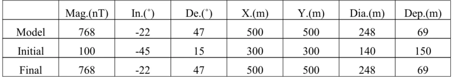
Table 3.1: Joint inversion of magnetic field and analytic signal for model 1... 49
Table 3.2: Joint inversion of magnetic field and analytic signal for model 2... 52
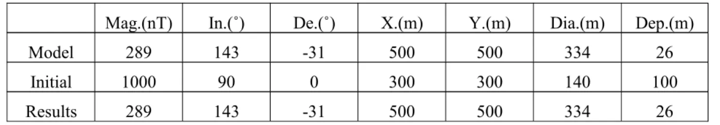
Table 3.3: Joint inversion of magnetic field and analytic signal for model 3... 55
Table 3.4: Joint inversion of magnetic field and analytic signal for model 4... 58
Table 5.1: Model 1 (a vertical cylinder at an intermediate depth with an inclination and a declination close to the geomagnetic inclination and declination contaminated with 50nT Gaussian noise): joint inversion of magnetic field and analytic signal (JIMA), magnetic field inversion (MFI) and analytic signal inversion (ASI)...75
Table 5.2: Model 2 (a vertical cylinder at an intermediate depth with an inclination and a declination differing from the geomagnetic inclination and declination contaminated with 50nT Gaussian noise): joint inversion of magnetic field and analytic signal (JIMA), magnetic field inversion (MFI) and analytic signal inversion (ASI)...78
Table 5.3: Model 3 (a shallow large diameter vertical cylinder with an inclination and a declination differing from the geomagnetic inclination and declination contaminated with 50nT Gaussian noise): joint inversion of magnetic field and analytic signal (JIMA), magnetic field inversion (MFI) and analytic signal inversion (ASI)...81
Table 5.4: Model 4 (a deep small diameter vertical cylinder similar to a vertical dipole with an inclination and a declination close to the geomagnetic inclination and declination contaminated with 50nT Gaussian noise): joint inversion of magnetic field and analytic signal (JIMA), magnetic field inversion (MFI) and analytic signal inversion (ASI)...84
Table 5.5: Model 5 (a vertical cylinder at an intermediate depth with an inclination and a declination close to the geomagnetic inclination and declination contaminated with 20nT Gaussian noise plus a plane regional): joint inversion of magnetic field and analytic signal (JIMA), magnetic field inversion (MFI) and analytic signal inversion (ASI)...89
Table 5.6: Model 6 (a vertical cylinder at an intermediate depth with an inclination and a declination differing from the geomagnetic inclination and declination contaminated with 20nT Gaussian noise plus a plane regional): joint inversion of magnetic field and analytic signal (JIMA), magnetic field inversion (MFI) and analytic signal inversion (ASI)...92 Table 5.7: Model 7 (a shallow large diameter vertical cylinder with an inclination and a declination differing from the geomagnetic inclination and declination contaminated with 20nT Gaussian noise plus a plane regional): joint inversion of magnetic field and analytic signal (JIMA), magnetic field inversion (MFI) and analytic signal inversion (ASI)...95 Table 5.8: Model 8 (a deep small diameter vertical cylinder similar to a vertical dipole with an inclination and a declination close to the geomagnetic inclination and declination contaminated with 20nT Gaussian noise plus a plane regional): joint inversion of magnetic field and analytic signal (JIMA), magnetic field inversion (MFI) and analytic signal inversion (ASI)... 98 Table 5.9: Model 9 (two vertical cylinders at an intermediate depth with an inclination and a declination close to the geomagnetic inclination and declination contaminated with 20nT Gaussian noise): joint inversion of magnetic field and analytic signal (JIMA), magnetic field inversion (MFI) and analytic signal inversion (ASI): joint inversion of magnetic field and analytic signal (JIMA), magnetic field inversion (MFI) and analytic signal inversion (ASI)... 103 Table 5.10: Model 10 (two vertical cylinders at an intermediate depth with an inclination and a declination differing from the geomagnetic inclination and declination contaminated with 20nT Gaussian noise): joint inversion of magnetic field and analytic signal (JIMA), magnetic field inversion (MFI) and analytic signal inversion...107 Table 5.11: Model 11 (two shallow large diameter vertical cylinders with an inclination and a declination differing from the geomagnetic inclination and declination contaminated with 20nT Gaussian noise): joint inversion of magnetic field and analytic signal (JIMA), magnetic field inversion (MFI) and analytic signal inversion (ASI)...111 Table 5.12: Model 12 (two deep small diameter vertical cylinders similar to a vertical dipole with an inclination and a declination close to the geomagnetic inclination and declination contaminated with 20nT Gaussian noise): joint inversion of magnetic field and analytic signal (JIMA), magnetic field inversion (MFI) and analytic signal inversion (ASI)...115
Table 5.13: AE-1: Initial and final parameters of joint inversion of magnetic field and analytic signal...122 Table 5.14: AE-2: Initial and final parameters of joint inversion of magnetic field and analytic signal...125
LIST
LIST
LIST
LIST OF
OF
OF
OF FIGURES
FIGURES
FIGURES
FIGURES
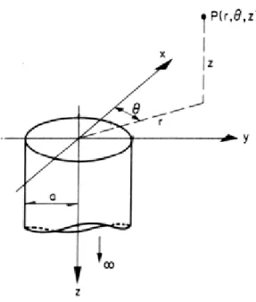
Figure 1.1: Model of an idealized kimberlite magnetic system illustrating the relationships between crater, diatreme and hypabyssal facies rocks. The diatreme root zone is composed primarily of hypabyssal rocks (After Mitchell, 1986)... 2 Figure 1.2: Relations between the remanent magnetization and induced magnetization when the total magnetization is known... 4 Figure 1.3: Geometry relationship of magnetic elements. Inclination (I) is the angle between the magnetic field vector and the local horizontal plane of the Earth. Declination (D) is the angle between the magnetic field projections to the Earth's surface and geographic north... 8 Figure 1.4: Relationship between types of magnetizations. Total magnetization is vector sum of induced magnetization and remanent magnetization... 9 Figure 1.5 Arrangements of atoms or dipole moments within or without the magnetic field: (a) is the arrangement of atoms of magnetizable material without the magnetic field; (b) is the arrangement of dipole moments without the magnetic field; (c) is the arrangement of atoms of magnetizable material within the magnetic field; (d) is the arrangement of dipole moments within the magnetic field... 10 Figure 1.6: Polarity of the Earth's magnetic field as a function of geological time. The paleomagnetic record is less detailed than the sea-floor data. Through the Cambrian to the Permian the field was mostly reversed, Triassic through Cretaceous mostly normal, and about half and half in the recent Cenozoic. (Macnae, 1995)...14 Figure 2.1: Geometry of semi-infinite vertical cylinder...21 Figure 2.2: Flow chart for the analytic signal computation...28 Figure 2.3: Model 1: magnetic field anomaly and its analytic signal. X-axes is directed to the east and Y-axes is directed to the north. (a) Total-field magnetic anomaly, (b) analytic signal computed using the Fourier transform method, (c) analytic signal computed using the finite difference method... 30 Figure 2.4: Model 2: magnetic field anomaly and its analytic signal for model. X-axes is directed to the east and Y-axes is directed to the north. (a) Total-field magnetic anomaly, (b)
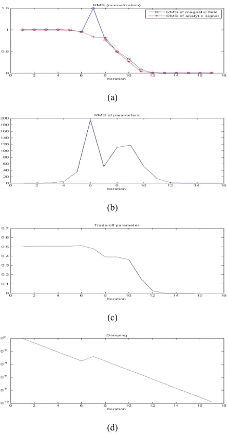
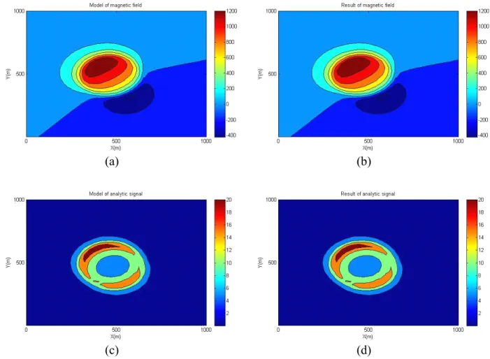
analytic signal computed using the Fourier transform method, (c) analytic signal computed using the finite difference method... .32 Figure 2.5: Model 3: magnetic field anomaly and its analytic signal. X-axes is directed to the east and Y-axes is directed to the north. (a) Total-field magnetic anomaly, (b) analytic signal computed using the Fourier transform method, (c) analytic signal computed using the finite difference method... 34 Figure 2.6: Model 4: magnetic field anomaly and its analytic signal. X-axes is directed to the east and Y-axes is directed to the north. (a) Total-field magnetic anomaly, (b) analytic signal computed using the Fourier transform method, (c) analytic signal computed using the finite difference method... 36 Figure 3.1: Flow chart for joint inversion computation...48 Figure 3.2: Model 1: joint inversion of magnetic field and analytic signal. X-axes is directed to the east and Y-axes is directed to the north. (a) Modeled total-field magnetic anomaly, (b) total magnetic field response to the inverted model, (c) modeled analytic signal, (d) analytic signal response to the inverted model... 50 Figure 3.3: Model 1: (a) data misfits of magnetic field and analytic signal respectively, (b) parameter changes, (c) trade-off parameter, and (d) damping factor... 51 Figure 3.4: Model 2: joint inversion of magnetic field and analytic signal. X-axes is directed to the east and Y-axes is directed to the north. (a) Modeled total-field magnetic anomaly, (b) total magnetic field response to the inverted model, (c) modeled analytic signal, (d) analytic signal response to the inverted model... 53 Figure 3.5: Model 2: (a) data misfits of magnetic field and analytic signal respectively, (b) parameter changes, (c) trade-off parameter, and (d) damping factor... 54 Figure 3.6: Model 3: joint inversion of magnetic field and analytic signal. X-axes is directed to the east and Y-axes is directed to the north. (a) Modeled total-field magnetic anomaly, (b) total magnetic field response to the inverted model, (c) modeled analytic signal, (d) analytic signal response to the inverted model... 56 Figure 3.7: Model 3: (a) data misfits of magnetic field and analytic signal respectively, (b) parameter changes, (c) trade-off parameter, and (d) damping factor... 57
Figure 3.8: Model 4: joint inversion of magnetic field and analytic signal. X-axes is directed to the east and Y-axes is directed to the north. (a) Modeled total-field magnetic anomaly, (b) total magnetic field response to the inverted model, (c) modeled analytic signal, (d) analytic signal response to the inverted model... 59 Figure 3.9: Model 4: (a) data misfits of magnetic field and analytic signal respectively, (b) parameter changes, (c) trade-off parameter, and (d) damping factor... 60 Figure 4.1: Geometry relationship between induced and remanent magnetizations... 63 Figure 4.2: Screen shot of the interface for EM1DFM...66 Figure 4.3: Inversion result of the semi-infinite prim model using EM1DFM software and synthetic data (top) and 20 recovered 1D models of conductivity and susceptibility concatenated into a 2D cross section under the survey line. True model: an outcropping vertical semi-infinite prism embedded in a homogeneous medium. Conductivity and susceptibility of the prism are 0.01 S/m and 0.1 SI units respectively, and conductivity and susceptibility of the background are 0.0001 S/m and 0 SI units. The reference models are a homogeneous half space of conductivity and susceptibility (a) 0.01 S/m and 0.1 SI units and (b) 0.0001 S/m and 0.0 SI units respectively...69 Figure 4.4: Inversion result of the semi-infinite prim model using EM1DFM software and synthetic data (top) and 20 recovered 1D models of conductivity and susceptibility concatenated into a 2D cross section under the survey line. True model: a vertical semi-infinite prism at 20m depth, embedded in a homogeneous medium. Conductivity and susceptibility of the prism are 0.01 S/m and 0.1 SI units respectively, and conductivity and susceptibility of the background are 0.0001 S/m and 0 SI units. The reference models are a homogeneous half space of conductivity and susceptibility (a) 0.01 S/m and 0.1 SI units and (b) 0.0001 S/m and 0.0 SI units respectively...70 Figure 5.1: Model 1 (a vertical cylinder at an intermediate depth with an inclination and a declination close to the geomagnetic inclination and declination contaminated with 50nT Gaussian noise): 2D contours of the models and inversion results... 75
Figure 5.2: Model 1 (a vertical cylinder at an intermediate depth with an inclination and a declination close to the geomagnetic inclination and declination contaminated with 50nT Gaussian noise): convergence plots...77 Figure 5.3: Model 2 (a vertical cylinder at an intermediate depth with an inclination and a declination differing from the geomagnetic inclination and declination contaminated with 50nT Gaussian noise): 2D contours of the models and inversion results... 78 Figure 5.4: Model 2 (a vertical cylinder at an intermediate depth with an inclination and a declination differing from the geomagnetic inclination and declination contaminated with 50nT Gaussian noise): convergence plots...80 Figure 5.5: Model 3 (a shallow large diameter vertical cylinder with an inclination and a declination differing from the geomagnetic inclination and declination contaminated with 20nT Gaussian noise): 2D contours of the models and inversion results... 81 Figure 5.6: Model 3 (a shallow large diameter vertical cylinder with an inclination and a declination differing from the geomagnetic inclination and declination contaminated with 20nT Gaussian noise): convergence plots...83 Figure 5.7: Model 4 (a deep small diameter vertical cylinder similar to a vertical dipole with an inclination and a declination close to the geomagnetic inclination and declination contaminated with 20nT Gaussian noise): 2D contours of the models and inversion results...84 Figure 5.8: Model 4 (a deep small diameter vertical cylinder similar to a vertical dipole with an inclination and a declination close to the geomagnetic inclination and declination contaminated with 20nT Gaussian noise): convergence plots... 86 Figure 5.9: Model 5 (a vertical cylinder at an intermediate depth with an inclination and a declination close to the geomagnetic inclination and declination contaminated with 20nT Gaussian noise plus a plane regional): 2D contours of the models and inversion results... 89 Figure 5.10: Model 5 (a vertical cylinder at an intermediate depth with an inclination and a declination close to the geomagnetic inclination and declination contaminated with 20nT Gaussian noise plus a plane regional): convergence plots... 91
Figure 5.11: Model 6 (a vertical cylinder at an intermediate depth with an inclination and a declination differing from the geomagnetic inclination and declination contaminated with 20nT Gaussian noise plus a plane regional): 2D contours of the models and inversion results... 92 Figure 5.12: Model 6 (a vertical cylinder at an intermediate depth with an inclination and a declination differing from the geomagnetic inclination and declination contaminated with 20nT Gaussian noise plus a plane regional): convergence plots... 94 Figure 5.13: Model 7 (a shallow large diameter vertical cylinder with an inclination and a declination differing from the geomagnetic inclination and declination contaminated with 20nT Gaussian noise plus a plane regional): 2D contours of the models and inversion results... 95 Figure 5.14: Model 7 (a shallow large diameter vertical cylinder with an inclination and a declination differing from the geomagnetic inclination and declination contaminated with 20nT Gaussian noise plus a plane regional): convergence plots... 97 Figure 5.15: Model 8 (a deep small diameter vertical cylinder similar to a vertical dipole with an inclination and a declination close to the geomagnetic inclination and declination contaminated with 20nT Gaussian noise plus a plane regional): 2D contours of the models and inversion results... 98 Figure 5.16: Model 8 (a deep small diameter vertical cylinder similar to a vertical dipole with an inclination and a declination close to the geomagnetic inclination and declination contaminated with 20nT Gaussian noise plus a plane regional): convergence plots... 100 Figure 5.17: Model 9 (two vertical cylinders at an intermediate depth with an inclination and a declination close to the geomagnetic inclination and declination contaminated with 20nT Gaussian noise): 2D contours of the models and inversion results... 104 Figure 5.18: Model 9 (two vertical cylinders at an intermediate depth with an inclination and a declination close to the geomagnetic inclination and declination contaminated with 20nT Gaussian noise): convergence plots...106 Figure 5.19: Model 10 (two vertical cylinders at an intermediate depth with an inclination and a declination differing from the geomagnetic inclination and declination contaminated with 20nT Gaussian noise): 2D contours of the models and inversion results...108
Figure 5.20: Model 10 (two vertical cylinders at an intermediate depth with an inclination and a declination differing from the geomagnetic inclination and declination contaminated with 20nT Gaussian noise): convergence plots... 110 Figure 5.21: Model 11 (two shallow large diameter vertical cylinders with an inclination and a declination differing from the geomagnetic inclination and declination contaminated with 20nT Gaussian noise): 2D contours of the models and inversion results... 112 Figure 5.22: Model 11 (two shallow large diameter vertical cylinders with an inclination and a declination differing from the geomagnetic inclination and declination contaminated with 20nT Gaussian noise): convergence plots...114 Figure 5.23: Model 12 (two deep small diameter vertical cylinders similar to a vertical dipole with an inclination and a declination close to the geomagnetic inclination and declination contaminated with 20nT Gaussian noise): 2D contours of the models and inversion results.. 116 Figure 5.24: Model 12 (two deep small diameter vertical cylinders similar to a vertical dipole with an inclination and a declination close to the geomagnetic inclination and declination contaminated with 20nT Gaussian noise): convergence plots...118 Figure 5.25: Aeromagnetic map (public domain) from a region of Ekati, Lac de Gras. The locations of AE-1 and AE-2 are marked on the map...120 Figure 5.26: AE-1: joint inversion of magnetic field and analytic signal, X-axis is directed to the east and Y-axis is directed to the north: (a) observed field magnetic data, (b) total-field magnetic response to the modeled pipe, (c) computed analytic signal data from total-total-field data, (b) analytic signal response to the modeled pipe... 122 Figure 5.27: AE-1: (a) data misfits of magnetic field and analytic signal respectively, (b) parameter changes, (c) trade-off parameter, and (d) damping factor... 123 Figure 5.28: AE-2: joint inversion of magnetic field and analytic signal, X-axis is directed to the east and Y-axis is directed to the north: (a) observed field magnetic data, (b) total-field magnetic response to the interpreted model, (c) computed analytic signal data from the total-field data, (d) analytic signal response to the interpreted model...125 Figure 5.29: AE-2: (a) data misfits of magnetic field and analytic signal respectively, (b) parameter changes, (c) trade-off parameter, and (d) damping factor... 126
LIST
LIST
LIST
LIST OF
OF
OF
OF SYMBOLS
SYMBOLS
SYMBOLS
SYMBOLS AND
AND
AND
AND ABBREVIATIONS
ABBREVIATIONS
ABBREVIATIONS
ABBREVIATIONS
f Total-field magnetic anomaly
g Analytic signal tot J� Total magnetization i J� Induced magnetization r J� Remanent magnetization tot
J Intensity of total magnetization
i
J Intensity of induced magnetization
r
J Intensity of remanent magnetization
tot
I Inclination of total magnetization
i
I Inclination of induced magnetization
r
I Inclination of remanent magnetization
tot
D Declination of total magnetization
i
D Declination of induced magnetization
r
D Declination of remanent magnetization
Q Königsberger ratio
κ Magnetic susceptibility
µ Magnetic permeability
0
µ Magnetic permeability of vacuum
σ Electric conductivity
TM Total magnetization
RM Remanent magnetization
JIMA Joint inversion of magnetic field and analytic signal MFI Magnetic field inversion
ASI Analytic signal inversion Mag. Total magnetization intensity
In. Total inclination of the magnetic field De. Total declination of the magnetic field Dia. Diameter of the cylinder
Dep. Depth of the cylinder RMS Root mean squares error Dep. Depth of the cylinder
β Trade-off parameter
λ Damping factor
Nor Normalization factor SI International system
INTRODUCTION
INTRODUCTION
INTRODUCTION
INTRODUCTION
Diamond is the fifth mineral in economic importance after iron, gold, copper and zinc
(Baumier, 1993). The diamond is generally found in two types of rock: kimberlite and lamproite. The total volume of known kimberlite in the world is more than 5,000 cubic kilometers and lamprophyre in the world is less than 100 cubic kilometers (Mitchell and Bergman, 1991). Most of diamonds are extracted from kimberlite rocks.The definition for kimberlite was present by Mitchell (1986): inequigranular alkalic peridotites containing rounded and corroded megacrysts of olivine, phlogopite, magnesian ilmenite and pyrope set in fine grained groundmass of second generation euhedral olivine and phlogopite together with primary and secondary diamond. The surrounding rock of kimberlite can be any sedimentary, metamorphic or igneous. Mitchell (1986) provided an idealized kimberlite model (Figure 1.1) that illustrates the relationships between crater, diatreme and hypabyssal facies rocks. The diatreme root zone is composed primarily of hypabyssal rocks. The diameter of kimberlite pipe is from a few meters to hundreds of meters, and the depth extent is from a few meters to thousands of meters.
Macnae (1995) describes the geometry of kimberlite pipe: “kimberlites tend to have circular, ellipsoidal or kidney shaped shallow expressions in plan. The least eroded pipes (generally larger in surface area) will have shallower dips at the pipe walls than more deeply eroded pipes. Geophysical modeling should not require a non-vertical dip for the axes of a pipe. Blind secondary or satellite pipes on the other hand may, however, cause response asymmetries. ” The classical model of a pipe is a carrot shaped or conical geometry with steeply dipping walls and diameter vanishing with increasing depth (Skinner, 1986) as in Figure 1.1.
Figure 1.1: Model of an idealized kimberlite magnetic system illustrating the relationships between crater, diatreme and hypabyssal facies rocks. The diatreme root zone is composed primarily of hypabyssal rocks (After Mitchell, 1986).
The magnetic properties are an important feature of kimberlite, because the magnetism of igneous rocks is larger than metamorphic rock or sedimentary rock generally. The existing geophysical literature in rock magnetism (Clark, 1983; Hargraves, 1989) shows that the kimberlite magnetic response is mainly caused by the direction and amplitude of remanent magnetization (RM in brief for the remaining of the thesis). For example, Hargraves (1989) The magnetic properties are an important feature of kimberlite, because the magnetism of igneous
rocks is larger than metamorphic rock or sedimentary rock generally. The existing geophysical literature in rock magnetism (Clark, 1983; Hargraves, 1989) shows that the kimberlite magnetic response is mainly caused by the direction and amplitude of remanent magnetization (RM in brief for the remaining of the thesis). For example, Hargraves (1989) published extensive paleomagnetic results over kimberlites in Southern Africa, and determined that RM was very consistent in direction within each sampled pipe.
Because of the magnetic properties of kimberlite, magnetic method is one of the most useful geophysical techniques to accurately determine the geometrical and magnetic properties, such as pipe shape, depth to top, magnetization. The magnetics show not only high sensitivity to kimberlite occurrence, but also it is relatively low cost and highly efficient, especially the airborne magnetics.
Magnetic interpretation provides information about the magnetization, location and size of the kimberlite pipe. A crucial parameter of kimberlite magnetic interpretation is the RM which dominates the classification of kimberlite, but the presence of RM can pose severe challenges to the quantitative interpretation of magnetic data by skewing or laterally shifting magnetic anomalies relative to the subsurface source (Haney and Li, 2002).
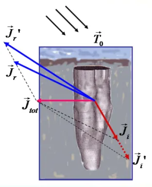
When the strong RM is present, the magnetic data is responding to total magnetization (TM in brief for the remaining of the thesis), which is consisted of a variety set of induced magnetization (IM in brief for the remaining of the thesis) and RM.However, the RM cannot be estimated directly or separated from the TM just utilizing the magnetic interpretation. Most of the methods use the mathematical relationships or direction bias to estimation the RM, such as minimizing the amplitude of RM. These methods can't estimate RM with certainty, because the RM not only biases the direction of TM but also change its magnitude. Figure 1.2 shows an example to explain this problem. If the TM is known, both magnitude and direction of RM are changed ( J�r changes to the J�r') when the magnitude of IM changes ( J�i changes to the J�i'). Therefore, the magnitude of IM or susceptibility must be known when the remanent magnetization has to be separated from the TM.
Figure 1.2: Relations between the remanent magnetization and induced magnetization when the total magnetization is known.
The objective of my thesis is to determine the RM and geometrical properties of kimberlite pipe. Furthermore, the magnetic interpretation method must be stable in presence of different typical noises.
To achieve this objective, I use a two-step strategy to interpret the magnetic data. The first step is to determine the TM from the total magnetic data in presence of strong RM. The second step is to obtain the magnetic susceptibility and then to separate the RM from the TM.
A three-dimensional (3D) parametric inversion algorithm was developed to determine the TM and geometrical properties of kimberlite pipe by using the magnetic total-field anomaly and its analytic signal in presence of strong RM. In general magnetic interpretation, the direction of magnetization is identical to the one of the geomagnetic field. However, the strong RM changes the direction of magnetization and generates the "false targets". The parametric inversion is a mean to solve this problem, because the direction of magnetization is independent on the geomagnetic field that is one of parameters to be interpreted.
For the interpretation of magnetic survey data collected over kimberlite, the parametric inversion assumes that a single magnetic body is present in selected area. However, the magnetic
anomaly can be affected with geological and processing noise, regional anomaly, interfering anomalies from other magnetic bodies. Thus the inversion algorithm needs to overcome those effects. The analytic signal is therefore used to improve interpretation of the magnetic data, because its sensitivity is different to total-field magnetic data in presence of noise. The joint inversion of the total magnetic field and the analytic signal is superior over the separated inversion of each set of data. It increases the resolution and stability of the results. The inversion algorithm uses Gauss-Newton method solved by singular value decomposition and Marquardt’s method.
As mentioned above, the RM cannot be estimated uniquely, unless the susceptibility is known. Traditionally, the RM or susceptibility of minerals and rocks are measured from orientated cores and active source experiments. However, these methods are not always feasible and have limitations because of its cost and they are time consuming (Shearer, 2005). Fortunately, the susceptibility can be estimated by using electromagnetic method, which is not affected by RM. The 1D inversion of EM data proposed by Zhang and Oldenburg (1996) is used to estimate the magnetic susceptibility and the electric conductivity. Then, the RM can be separated from the TM according to the relationship between the RM, susceptibility and TM.
In order to verify the joint inversion of magnetic field and analytic signal, four different synthetic models are used. The first model is a vertical cylinder at an intermediate depth, an inclination and a declination close to the geomagnetic inclination and declination. The second model is an intermediate depth vertical cylinder with inclination and declination differing with the Earth's field inclination and declination. The third model is a shallow large diameter vertical cylinder with inclination and declination differing with the Earth's field inclination and declination. The fourth model is a deep small diameter vertical cylinder similar to a vertical dipole, its inclination closes to the vertical and its declination closes to the Earth's field declination.
The main scientific contributions from my thesis are: (1) the analytic signal is derived by using Fourier transform method; (2) a joint inversion of magnetic field and analytic signal is implemented, which adds stability and precision to the solution; (3) the magnetic technique and EM technique are combined to separate the RM from the TM.
There are five chapters in this thesis:
Chapter 1 is an overview of the magnetic techniques. I introduce the history and concepts of magnetics and illustrate the main interpretation methods including the one with strong RM. Then I present development of magnetic technique for detecting the kimberlite.
Chapter 2 describes the analytic signal methodology that contains the basic principle of analytic signal and its calculations. First, I introduce the theory of analytic signal and the expression of its absolute value. Then, I review the expression of magnetic total-field anomaly due to a vertical right circular cylinder. After that, I introduce the computational method to obtain the analytic signal by Fourier transform. Finally, I illustrate the algorithm with synthetic examples.
Chapter 3 describes the inversion methodology that contains the theory and computation of joint inversion of magnetic field and analytic signal. Firstly, I introduce the inversion theory to solve the general problem. Then, I present the specific computation and structure diagram to complete the joint inversion of the magnetic total-field anomaly and its analytic signal due to a vertical right circular cylinder with arbitrary polarization. Finally, I illustrate the algorithm with synthetic examples.
Chapter 4 examines how to resolve the RM. I first introduce the RM computation from the TM and IM. Then the frequency EM survey is proposed to estimate the magnetic susceptibility. Finally, I illustrate the algorithm with synthetic examples.
Chapter 5 examines the performance of the joint inversion using synthetic tests. It discusses the advantages and usability of joint inversion of magnetic field and analytic signal. First, all model responses of total-field magnetic data and its analytic signal are contaminated with Gaussian noise only. Then, the regional noise is added. After that, I also consider a model response generated by two pipes and contaminated with Gaussian noise. Finally, a field example is used to illustrate the usability of joint inversion of magnetic field and analytic signal.
CHAPTER
CHAPTER
CHAPTER
CHAPTER 1
1
1
1
BACKGROUND
BACKGROUND
BACKGROUND
BACKGROUND
The purpose of this chapter is to briefly overview the developments magnetic techniques. Firstly, I introduce the history and concepts of magnetics. Then, I illustrate main methods of magnetic interpretation. After that, I introduce methods to interpret magnetic data with strong RM. Lastly, I present development of magnetic technique for detecting the kimberlite.
1.1
1.1
1.1
1.1
Concept
Concept
Concept
Concept of
of
of
of magnetics
magnetics
magnetics
magnetics
The magnetism was used for navigation as early as several centuries B.C in China, and recognized Earth's field by 11th century. In end of 12th century, the magnetic compass was
developed in Europe.
The magnetics method has become a geophysical exploration technique
first studied by occidental scientists since William Gilbert (1544-1603), who is regarded by some as the father of magnetism and published "De Magnete" in 1960. He carved sphere from lodestone and found field similar to Earth's. In the middle of seventeen century, Swedish geophysicists have used magnetic compass to detect magnetite. Until 1843, Von Wrede first used variations in the field to locate deposits of magnetic ore. In 1879, Thalen examined magnetite deposits with magnetics. The magnetics is used variations of the magnetic field were used to map the distribution of magnetic materials buried underground. Schmidt invented the quartz blade magnetometer and since then magnetics have been used for mineral exploration at large in 1915. In the 1940s, the vertical component of magnetic field has been measured. After World War Second, the Fluxgate magnetometer was invented that made the aeromagnetic measurement possible, and aeromagnetic measurement became popular in geophysical exploration later. After that, Proton-precession magnetometers and Optically pump alkali-vapor magnetometers came out, caused the measurements more accurate. At present, the digital technique is using in recording and processing of magnetic data.1.1.1
1.1.1
1.1.1
1.1.1 Magnetic
Magnetic
Magnetic
Magnetic elements
elements
elements
elements
In general, the magnetic field could be described by rectangular coordinates. Supposed that origin of coordinate is observation point, x-axes directs north, y-axes directs east, z-axes directs the Earth’s core. The magnetic features of this point can be expressed by seven magnetic
elements. Figure 1.2 presents the geometrical relationship of magnetic elements, and the expressions of the relationships of magnetic elements are written as follow:
Figure 1.3: Geometry relationship of magnetic elements. Inclination (I) is the angle between the magnetic field vector and the local horizontal plane of the Earth. Declination (D) is the angle between the magnetic field projections to the Earth's surface and geographic north.
2 2 2 2 2 2
cos ; sin ; tan /
cos ; sin ; tan /
T H Z X Y Z X H D Y H D D Y X H T I Z T I I Z H ⎧ = + = + + ⎪ = = = ⎨ ⎪ = = = ⎩ (1.2.1-1)
where, T is the magnetic intensity vector, H is the horizontal component of T, Z is the vertical component of T, X is the x axes component of T, Y is the y axes component of T, I is the inclination which is the angle between the magnetic field vector and the horizontal plane. D is the declination, which is the angle between Geographical meridional plane and the horizontal component of magnetic field vector. The unit of T, H, X, Y, Z is Tesla (T) in SI system and gamma (γ ) in cgs system ( 2 / 1 1T = Wb m , nT 9T 10 1 1γ = = − ).
According to the expressions of magnetic elements, all the elements can be expressed by arbitrarily three elements. The magnetic intensity vector, inclination and declination are generally used in magnetic exploration.
1.1.2
1.1.2
1.1.2
1.1.2 Magnetization
Magnetization
Magnetization
Magnetization
Material in magnetic field produces magnetic phenomenon calls magnetization. It is a function of location and varies from point to point (Blakeley, 1996). Different materials in the same magnetic field or same materials in the different magnetic field are magnetized differently. Magnetization can be defined according to the following equation:
= m J V ∆
∑
� � (1.2.2-1) where, J� represents magnetization, m� is the individual magnetic dipole moment, ∆Vrepresents summation volume of dipole moments.
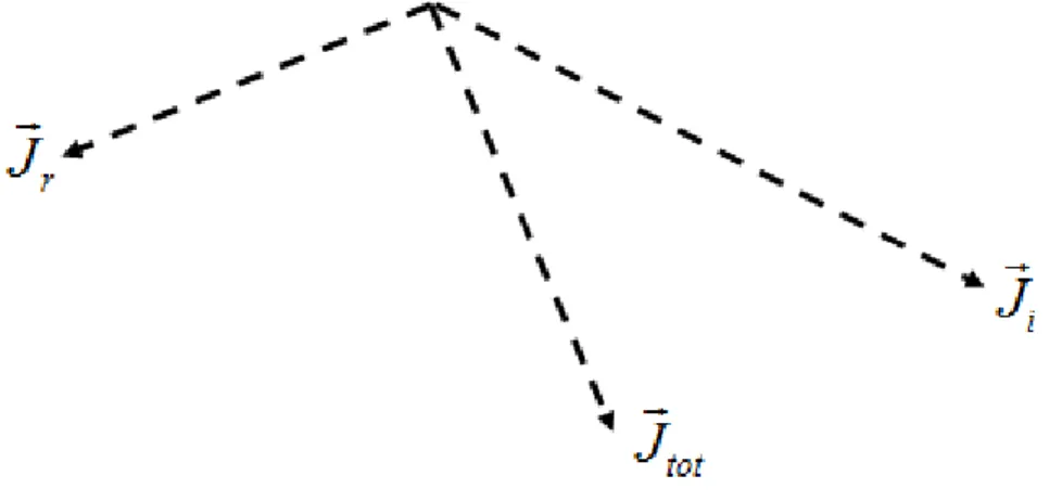
Macro to see, the magnetization is called total magnetization ( J�tot ) is composed of induced magnetization (J�i) and remanent magnetization (J�r). Figure 1.3 shows the relationship of magnetizations which is expressed that:
Figure 1.4: Relationship between types of magnetizations. Total magnetization is vector sum of induced magnetization and remanent magnetization.
tot i r
J� = J� +J� (1.2.2-2)
The unit of magnetization is ampere/meter (A/m) in SI system and gauss (G) in cgs system (1G=103A/m).
1.1.3
1.1.3
1.1.3
1.1.3 Induced
Induced
Induced
Induced magnetization
magnetization
magnetization
magnetization
The induced magnetization is the material magnetic polarization in reaction to an external
magnetic field. In the subsurface, magnetic domains in magnetically susceptible mineral and rocks act as a collection of small magnets, with each domain having a dipole moment. In the absence of an external magnetic field, the individual dipole will be randomly orientated. With this arbitrary orientation, the net magnetization is zero (Shearer, 2005).Figure 1.5 Arrangements of atoms or dipole moments within or without the magnetic field: (a) is the arrangement of atoms of magnetizable material without the magnetic field; (b) is the arrangement of dipole moments without the magnetic field; (c) is the arrangement of atoms of magnetizable material within the magnetic field; (d) is the arrangement of dipole moments within the magnetic field.
Magnetic susceptibility is the physical property describing the ability of materials to be magnetized into an inducing external field. “The physics of induced internal magnetization in small fields such as the Earth’s is mathematically expressed by a linear relationship” (Macnae 1995). The expression of relationship is written as followed:
0
i
J =κT
(1.2.3-1) where, J is the induced magnetization, κ is the magnetic susceptibility andi T is the0
external inducting magnetic field.
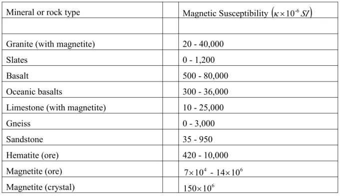
In general, the mineral magnetism is defined by susceptibility. Consequently, basic and ultrabasic rocks have the highest susceptibility, acid igneous and metamorphic rocks have intermediate to low values, and sedimentary rocks have very small susceptibilities in general (Chen, 2009). Sharma (1997) shows the list of magnetic susceptibility values for common mineral and rock types in Table 1.1.
Table 1.1: List of magnetic susceptibility values for common minerals and rocks.
Mineral or rock type Magnetic Susceptibility
(
-6SI)
10 ×
κ
Granite (with magnetite) 20 - 40,000
Slates 0 - 1,200
Basalt 500 - 80,000
Oceanic basalts 300 - 36,000
Limestone (with magnetite) 10 - 25,000
Gneiss 0 - 3,000 Sandstone 35 - 950 Hematite (ore) 420 - 10,000 Magnetite (ore) 4 10 7 × -14×106 Magnetite (crystal) 6 10 150×
Whole rock susceptibilities can considerably vary owing to a number of factors in addition to mineralogical composition. Susceptibilities depend upon the alignment and shape of the magnetic grains dispersed throughout the rock (Reynolds, 1997).
1.1.4
1.1.4
1.1.4
1.1.4 Remanent
Remanent
Remanent
Remanent magnetization
magnetization
magnetization
magnetization
Certain materials not only have atomic moments, but neighboring moments interact strongly with each other. Such materials are said to be ferromagnetic. The ferromagnetic materials have an ability to retain the magnetization in the absence of external magnetic field. This permanent magnetization is called remanent magnetization (Blakely, 1996).
The remanent magnetization is a function of quantity, atomic, crystallographic, chemical makeup, and grain size of the magnetic minerals. Small magnetic grains support strong, stable remanent magnetizations. It is also affected by the geologic, tectonic, and thermal history of the mineral or rock (Blakely, 1996). The various processed by which rocks can acquire a remanent magnetization are detailed in the table 1.2 (Shearer, 2005).
Table 1.2: Types of remanent magnetization (Shearer, 2005).
Remanent Magnetization Acronym Rock Types Description
Natural NRM ALL Summation of all remanent
magnetization components (primary and secondary).
Thermal TRM Igneous,
Metamorphic
Primary remanent magnetization acquired during cooling from a temperature above the Curie temperature in the presence of an external magnetic field.
Viscous VRM All Secondary remanent magnetization
acquired over time, related to thermal agitation and causes decay of primary remanent magnetization.
Depositional DRM Sedimentary Primary remanent magnetization acquired during deposition in the presence of an external field by the physical rotation of magnetic mineral particles. Usually occurs as grains settle out of water.
Post-depositional PDRM Sedimentary Acquired during post-depositional retention of interstitial grains.
Chemical CRM All Remanent magnetization acquired
during growth of magnetic minerals in presence of an external field. Includes growth by nucleation or replacement.
Isothermal IRM All Secondary remanent magnetization
acquired over a short time at one temperature in a strong, external field.
Natural remanence (NRM) is the main property to control the kimberlite magnetic responses. It is the phenomenon most studies by paleomagnetists (Figure 1.5) whose interest lies in ancient magnetic fields, specifically their intensity and direction (Macnae, 1995). TRM and CRM are two important causes of NRM.
Figure 1.6: Polarity of the Earth's magnetic field as a function of geological time. The paleomagnetic record is less detailed than the sea-floor data. Through the Cambrian to the Permian the field was mostly reversed, Triassic through Cretaceous mostly normal, and about half and half in the recent Cenozoic. (Macnae, 1995)
Commonly the amplitude of hard remanence measured by rock magnetists is larger than the amplitude of induced magnetism, and the Koningsberger ratio (Q) has been defined as the ration of remanent to induced response (Macnae, 1995). Usually the kimberlite breccias are characterized by a low (ranging from 0.2 - 0.8, rarely 2 - 3), however for the hypabyssal kimberlite type, the indicator displays remanence magnitudes of 4 to 6 (Dortman, 1984).
Viscous remanent magnetization (VRM) is an extremely important property to control the kimberlite magnetic responses. VRM is the continuing development of an internal remanent magnetic field parallel to the external field. The intensity of VRM if often a significant fraction of the NRM and induced magnetization, and may exceed either or both in amplitude. VRM intensities are quoted for continental samples; they vary from a few percent of the total NRM up to amplitudes equal to or greater than hard remanent magnetization. VRM will tend to increase
the fraction of the total internal magnetization that will be approximately parallel to the Earth's present field, and may explain why detected anomalies are of normal polarity even when quoted Q values such as those by Clark (1983) indicate that remanence should dominate (Macnae, 1995).
1.2
1.2
1.2
1.2 Magnetic
Magnetic
Magnetic
Magnetic interpretation
interpretation
interpretation
interpretation
Magnetic interpretation is an automatic numerical procedure that constructs a model of subsurface geology from measured magnetic data and other information, with the additional condition that input data are reproduced within a given error tolerance (Nabighian and al., 2005). In order to solve different problems, three interpretation methods were successfully developed: depth estimation, parametric inversion and physical property inversion. Shearer (2005) reviewed a variety of numerical interpretation approaches.
1.2.1
1.2.1
1.2.1
1.2.1 Depth
Depth
Depth
Depth estimation
estimation
estimation
estimation
Depth estimation techniques are initial and useful method to obtain a semi-quantitative representation of the source location. This type of technique initially presumes a regular geometric body shape (contacts, dikes, plates, cylinders and so on) in order to solve nonlinear inversion problems. The estimation parameters is vastly reduced that the problem is an over-determined Shearer (2005).
Naudy (1971) introduced a method to calculate profile over a vertical dike or thin plate by a matched filter, which is applied to observed and reduced-to-the-pole components. O'Brien (1972) introduced CompuDepth method, a frequency-domain technique that determines location and depth to 2D magnetic sources.
Hartman (1971) and Jain (1976) introduced Werner deconvolution method, that utilize total field as well as vertical and horizontal derivative information to estimate the depth, dip, horizontal position and susceptibility contrast of an assumed dike or interface source body. Phillips (1979) introduced ADEPT method, which estimates source parameters from an autocorrelation of an evenly sampled magnetic anomaly profile with dike or contact models.
Thompson (1982) introduced Euler Deconvolution method that solves Euler equation to find depth estimations based on a structural index and increasing window sizes. This method uses first order for each derivatives to determine location and depth for various simple targets, such as
sphere and cylinder, each characterized by specific structural index. Reid (1990) extended this method to 3D domain, offering a technique for analyzing mapped magnetic data. Nabighian and Hansen (2001) introduce an extended Euler deconvolution based on 3D Hilbert transform.
1.2.2
1.2.2
1.2.2
1.2.2 Parametric
Parametric
Parametric
Parametric inversion
inversion
inversion
inversion
Parametric inversion is a quantitative inversion technique for recovering the simple geometry of causative bodies that forward modeling. This method requires certain a prior information, such as a known magnetization direction. This type of nonlinear inversion solves an over-determined problem and recovers parameters for simple bodies, such as prisms and dikes (shearer, 2005).
Bhattacharyya (1980) introduced a 3D iterative method to characterize the magnetized region that fits the measured anomalous response of the subsurface. The horizontal dimensions of the rectangular blocks that comprise the model region are based on the height of observation surface, and the vertical extents of the blocks are adjusted to find a least squares fit between the observed and calculated field values. This method uses the RM to constrain the magnetization direction of each block.
Zeyen and Pous (1991) introduced 3D inversion method to recover parameters for the top and base of vertical rectangular prisms, susceptibility and RM. This method is strongly dependent on the initial model which is modeling by a mount of a prior information, that will restrict the solution to a subset of possible models and does not let the inversion recover a set of parameters that fall outside this model space. Therefor, this method is limited to areas where details about causative body geometry, parameter and property values are well known.
Wang and Hansen (1990) extended the CompuDepth method (O'Brien, 1972) to figure out the corners of 3D homogeneous polyhedral bodies. The depth and location of polyhedral vertices are described by a series of calculated coefficients. The method has the limitation in constructing causative bodies from discrete vertices, even though Wang and Hansen (1990) used other parametric inversion to improve the problem.
1.2.3
1.2.3
1.2.3
1.2.3 Physical
Physical
Physical
Physical property
property
property
property inversion
inversion
inversion
inversion
Physical property inversion is an inversion technique for recovering the subsurface distribution of a physical property, such as magnetic susceptibility (Li and Oldenburg, 1996). This type of linear or nonlinear inversion solves an under-determined problem and recovers parameters for the distribution of physical property.
Li and Oldenburg (1996) introduced a generalized magnetic inversion for distributions of susceptibility, which is useful in areas of multiple anomalies on a variety of scales. The method solves an underdetermined problem by minimizing a global objective function comprised of a model objective function and data misfit. The non-uniqueness of the solution, which is caused by underdetermined problem, is reduced by prior information and constraints (positivity, depth weighting, geologic reasonability).
Pilkington (1997) introduced a 3D inversion method that uses a preconditioned conjugate gradient method for computational efficiency to estimation the distribution of magnetic susceptibility.
Shearer and Li (2004) developed a 3D inversion method to recover the subsurface distribution of magnetic susceptibility. The method inverted amplitude of the anomalous magnetic field and total gradient data directly to recover the magnitude of magnetization without precise knowledge of its direction.
1.3
1.3
1.3
1.3
Magnetic
Magnetic
Magnetic
Magnetic interpretation
interpretation
interpretation
interpretation with
with
with
with strong
strong
strong
strong remanent
remanent
remanent
remanent magnetization
magnetization
magnetization
magnetization
The RM has hampered the magnetic interpretation for a long time, but has not received much attention for two reasons. First, the TM direction is similar to the orientation of the inducing field in the majority of exploration problems. The reason is that the direction of the RM is approximately collinear (aligned or antiparallel) with the current inducing field or the amplitude of the RM is weak. Second, the earlier interpretation techniques are weakly dependent on the TM direction, such as depth estimation techniques. However, RM is often strong and cannot be disregarded in numerous cases, such as archaeology, some mineral exploration, basement imaging in petroleum exploration, and crustal and planetary studies (Shearer, 2005).
Most of methods interpret the magnetic data in the presence of strong RM through direction estimation and exploitation of mathematical relationships, often utilizing quantities that have no or minimal dependence on magnetization direction.
Roest and Pilkington (1993) utilized the total gradient and pseudo gravity to estimate the TM direction and determine the location of source bodies using the properties of the magnetic anomaly. Haney and Li (2002) extracted the TM direction and dip from total field measurements using continuous wavelet transforms. Shearer and Li (2004) developed a 3D physical property inversion algorithm that utilized the minimal dependence on magnetization direction by quantities such as total gradient in presence of RM with Tikhonov regularization method to recover the subsurface distribution of magnetic susceptibility. Chemam (2006) and Chen (2009) utilized amplitude of magnetic anomaly and its analytic signal to do the parametric inversion using the model of vertical cylinder in presence of RM with Gauss-Newton method to recover the magnetic and geometrical properties of kimberlite pipe.
1.4
1.4
1.4
1.4 Magnetic
Magnetic
Magnetic
Magnetic technique
technique
technique
technique for
for detecting
for
for
detecting
detecting
detecting the
the
the
the kimberlite
kimberlite
kimberlite
kimberlite
Burley and Greenwood (1972) found magnetic anomalies over all known kimberlites in Lesotho. Macnae (1979) gave an example of an aeromagnetic survey that was flown by Geoterrex Ltd., of Ottawa, Canada. Nixon (1981) mentions that magnetic anomalies may occur within individual pipes, as in Letseng-la-Terae, Lesotho, indicating separate diamondiferous intrusions. Atkinson (1989) states that the variable and complex nature of magnetic responses found over kimberlites is more likely to reflect the nature of the body itself than the differential weathering of the pipe. Sarma (1999) used the ground magnetic vertical intensity contour map to map the Majhgawan kimberlite pipe near Panna in central India successfully.
Airborne magnetics and grounds magnetics are common techniques using in magnetic survey for kimberlite. The most cost-effective geophysical reconnaissance technique has been airborne magnetics (Macnae, 1995). Keating and Sailhac (2004) indicated that most kimberlites have a distinctive aeromagnetic signature that is a roughly circular anomaly in general, but the anomaly at ground level is more complex and it can have internal highs or be elongated. Therefore, most of pipes were first detected by means of an airborne reconnaissance survey.
The magnetic interpretation of kimberlite is to determine the nature remanent component, the viscous and induced components and geometry properties of anomaly. Paterson (1991) introduced the 3D Euler deconvolution to automatically locate circular anomalies, but this technique tends to generate a large number of "false targets". Keating (1995) introduced matched filter that is based on first-order regression analysis between a window of the gridded data and a typical target theoretical anomaly, but the filter dose not deal with low magnetic latitudes and strong magnetic remanence very well. Keating (2004) improved this method that changed window between the analytic signal of the observed magnetic field and the theoretical analytic signal of a magnetic vertical cylinder. Paulo (2007) introduced a technique based on joint analysis of analytic signal and Euler deconvolution. Cheman (2006) worked about the parametric and physical property inversion of magnetic field and analytic signal data due to the vertical right cylinder with arbitrary polarization in presence of remanence using the model of kimberlite pipe. He presented the RM to the inversion, and did the initial works for the separation the RM from the TM for the anomalies from the kimberlites. Chen (2009) continued and improved parametric and physical property inversion of magnetic field and analytic signal data due to the vertical right cylinder with arbitrary polarization in the presence of the remanence using the model of cylinder.
As discussed above, the results of magnetic interpretations always get the false targets. In order to reduce the "false targets", the other information must to be operated into the interpretation, such as geological (structural and tectonic), geochemical and other geophysical data (gravity, EM, resistivity, spectrometry).
CHAPTER
CHAPTER
CHAPTER
CHAPTER 2
2
2
2
ANALYTIC
ANALYTIC
ANALYTIC
ANALYTIC SIGNAL
SIGNAL
SIGNAL
SIGNAL METHODOLOGY
METHODOLOGY
METHODOLOGY
METHODOLOGY
The purpose of this chapter is to introduce the basic principle of analytic signal and derive for its calculation. First, I introduce the theory of analytic signal and the expression of absolute value of the analytic signal. Then, I review the expression of total magnetic field anomaly due to a vertical right circular cylinder. I then introduce the computational of analytic signal by Fourier transform. Lastly, I illustrate the algorithm with synthetic examples.
2.1
2.1
2.1
2.1
Introduction
Introduction
Introduction
Introduction
The analytic signal is computed from the gradients along the three axes of magnetic data. It is weakly dependent of the total magnetization direction. Nabighian (1972) computed the amplitude of the two-dimensional gradient vector from a given magnetic profile. The vertical derivative of magnetic field can be calculated from the horizontal derivative by Hilbert transforms. In 1984, Nabighian further developed the relationship between horizontal and vertical derivatives by Hilbert transforms that expanded method to three dimensions. Paine et al. (2001) examine the total gradient of the vertically integrated magnetic anomaly and vertical integration of the total gradient due to weak dependence on magnetization direction and both quantities processing the dimensions of the magnetic field.
The three-dimensional g� of a potential-field anomaly can be defined as follow:
, f f f g i j k x y z ⎛∂ ∂ ∂ ⎞ =⎜ + + ⎟ ∂ ∂ ∂ ⎝ ⎠ � � � � (2.1-1) where f is responses of magnetic field, and i� , �j , k� are unit vectors in the x, y, z directions respectively.
The absolute value of the analytic signal is defined as the square root of the sum of squared vertical and two horizontal derivatives of the total magnetic field anomaly. The expression of the analytic signal is written as follows:
2 2 2 f f f g g x y z ⎛ ⎞ ∂ ∂ ∂ ⎛ ⎞ ⎛ ⎞ = = ⎜ ⎟ +⎜ ⎟ +⎜ ⎟ ∂ ∂ ∂ ⎝ ⎠ ⎝ ⎠ ⎝ ⎠ � (2.1-2)