JOINT PRODUCTION, QUALITY CONTROL AND
MAINTENANCE POLICIES SUBJECT TO
QUALITY-DEPENDENT DEMAND
By
SAEED KHADANGI
THESIS PRESENTED TO ÉCOLE DE TECHNOLOGIE SUPÉRIEURE IN
PARTIAL FULFILLMENT OF A MASTER’S DEGREE WITH THESIS IN
AUTOMATED MANUFACTURING ENGINEERING
M.A.SC.
MONTREAL, NOVEMBER 25, 2019
ÉCOLE DE TECHNOLOGIE SUPÉRIEURE
UNIVERSITÉ DU QUÉBEC
©Tous droits réservés
Cette licence signifie qu’il est interdit de reproduire, d’enregistrer ou de diffuser en tout ou en partie, le présent document. Le lecteur qui désire imprimer ou conserver sur un autre media une partie importante de ce document, doit obligatoirement en demander l’autorisation à l’auteur.
BOARD OF EXAMINERS
THIS THESIS HAS BEEN EVALUATED BY THE FOLLOWING BOARD OF EXAMINERS:
Mr. Mustapha Ouhimmou, Thesis supervisor
Department of Systems Engineering, École de technologie supérieure
Mr. Ali Gharbi, co-supervisor
Department of Systems Engineering, École de technologie supérieure
Mr. Jean-Pierre Kenné, president of the board of examiners
Department of Mechanical Engineering, École de technologie supérieure
Mr. Armin Jabbarzadeh, member of the board of examiners
Department of Systems Engineering, École de technologie supérieure
THIS THESIS WAS PRESENTED AND DEFENDED
IN THE PRESENCE OF A BOARD OF EXAMINERS AND THE PUBLIC
ON "DEFENSE DATE"
ACKNOWLEDGMENTS
I would like to thank my fiance, Zinat, for all her support during the harsh days of winter 2019, working for us until midnight.
I would also like to express my gratitude to my research professors for their availability and valuable advice.
I wish to offer my thanks to Morad Assid and the other members of the Laboratory of Design and Control of Production Systems (A3430) at ÉTS University who helped me a lot in
finalizing this thesis.
Finally, I would like to thank my parents, my little brother, and friends for all their love sent to me.
POLITIQUES CONJOINTES DE PRODUCTION, DE CONTRÔLE DE QUALITÉ ET DE MAINTENANCE SOUMISES À UNE DEMANDE DE QUALITÉ
SAEED KHADANGI
RÉSUMÉ
Cette thèse vise à trouver une solution appropriée en utilisant les moyens de contrôle stochastiques optimaux pour un système de production non-fiable avec un contrôle de la qualité du produit et une demande dépendant de la qualité. Le système consiste en une seule machine produisant un seul type de produit (M1P1) sujet à des pannes et à des réparations aléatoires et devant satisfaire un taux de demande client non constant, qui répond à la qualité des pièces reçues. Étant donné que la machine produit avec un taux de produits non conformes, une inspection des produits est effectuée afin de réduire le nombre de pièces défectueuses pouvant être livrées au client. Cela se fait en continu et consiste à contrôler une fraction de la production. Les produits approuvés sont remis sur la chaîne de production, tandis que les mauvais produits sont jetés.
L’objectif visé par cette étude est de fournir un contrôle de la qualité et une politique de production optimale, qui maximise le revenu net composé du revenu brut, du coût des stocks, du coût des pénuries, du coût de l’inspection, du coût de la maintenance et du coût des pièces sans qualité. Les principales variables de décision sont le taux d'échantillonnage du système de contrôle de la qualité ainsi que seuil d'inventaire de produit fini. La fonction de demande réagit au niveau de qualité moyen sortant (AOQ) des produits finis. Dans le troisième chapitre de cette étude, les stratégies de maintenance préventive et de tarification dynamique sont ajoutées à la stratégie optimale, citée ci-dessus.
Pour atteindre les points optimaux de la politique, qui maximisent nos revenus de production nets, une approche de simulation est mise en œuvre à titre expérimental et ses résultats sont utilisés dans la méthodologie de la surface de réponse.
Pour mettre en œuvre le plan d’expérience (approche de la simulation) reflétant parfaitement les considérations du modèle, telles que son caractère continu et sa variété, une variable continue a été introduite pour la probabilité de défectuosité, fonctionnant avec l’âge de la machine jusqu’à la prochaine maintenance. Deuxièmement, afin de refléter l’effet du processus
de contrôle qualité qui se traduit par une qualité moyenne sortante plutôt que par une simple possibilité de défectuosité, cette fonction (AOQ) a été construite sur la base du comportement instantané de la fonction mentionnée ci-dessus en tant que variable indépendante. Troisièmement, en raison de l’utilisation des hypothèses de la théorie des clients potentiels pour créer une fonction de demande répondant au niveau de défectuosité fournie par le client (AOQ), une fonction continue réactive a été créée pour la demande, réagissant au niveau de qualité du produit en déterminant son taux. Finalement. Pour illustrer la politique de fabrication de la machine basée sur Hedging Point, une variable d’inventaire du produit fini a été introduite dans la conception de l’expérience.
En résumé, nous avons un système de production conçu de manière à ce que, en augmentant son âge (At), il soit possible d'accroître les possibilités de défectuosité et de réduire la demande
en unités de temps. Cette manière de procéder continue jusqu'à la prochaine action de maintenance du système, ce qui restaure tous les facteurs dans leurs conditions initiales. En utilisant l'approche de simulation d'optimisation, une expérience est conçue et mise en œuvre pour contrôler les variables de décision de la politique et maximiser la fonction objective du revenu net moyen (ANR). Les variables de décision sont statistiquement et pratiquement prises en compte, telles que le niveau d’inventaire (Z), la proportion d’inspection (F) et les seuils de PM (Mk ou Pk).
Mots-clés: Production system, optimal stochastic control, quality control, simulation,
experimental design, response surface methodology, quality dependent demand, prospect theory
JOINT PRODUCTION, QUALITY CONTROL AND MAINTENANCE POLICIES SUBJECT TO QUALITY-DEPENDENT DEMAND
SAEED KHADANGI
ABSTRACT
This thesis is a strive to find a proper solution, using the stochastic optimal control means for an unreliable production system with product quality control and quality-dependent demand. The system consists of a single machine producing a single product type (M1P1) subject to breakdowns and random repairs and must satisfy a non-constant rate of customer demand, which response to the quality of parts received. Since the machine produces with a rate of non-compliant products, an inspection of the products is made to reduce the number of bad parts that would deliver to the customer. It is done continuously and consists of controlling a fraction of the production. Approved products are put back on the production line, while bad products are discarded.
The intended objective of this study is to provide optimal quality control and production policy, which maximize the net revenue consisting of the gross revenue, the cost of inventory, the cost of shortage, the cost of the inspection, the cost of maintenance and the cost of no-quality parts. Main decision variables are the sampling rate of the quality control system as well as the threshold of finished product inventory. The demand function reacts to the average outgoing quality level (AOQ) of finished products. In the third chapter of this study, preventive maintenance and dynamic pricing policies are added up to the optimal policy, cited above. To achieve the optimal points of the policy, which maximize our net production revenue, a simulation approach is implemented as an experimental design and its results were used in response surface methodology.
To implement the experiment design (simulation approach) which thoroughly reflects model considerations such as its continuous nature and the variety, first, a continuous variable for the probability of defectiveness was introduced, functioning with the age of machine up until its next breakdown maintenance. Second, so as to reflect the effect of quality control process that results in Average Outgoing Quality rather than simple defectiveness possibility, this function (AOQ) was built based on instant behavior of mentioned function above as its independent variable. Third, due to the use of prospect theory assumptions in building a demand function that responds to the level of client delivered defectiveness (AOQ), a responsive continuous function was created for the demand, reacting to the level of product quality by determining it's needed per time amount. Finally. To illustrate the machine’s manufacturing policy based on Hedging Point, finished product inventory variable was introduced in the experiment design.
In a nutshell, we have a production system that has been designed in a way that by raising its age (At), leads to more possibility of defectiveness and less demand in time units. This manner
continuous up until the next maintenance action of the system, which restores all factors to their initial conditions. By use of the simulation approach of optimization an experiment is designed and implemented to control decision variables of the policy and maximize the objective function of average net revenue (ANR). Decision variables are statistically and
practically in the matter of consideration such as finished product inventory threshold (Z), the proportion of inspection (F) and PM thresholds (Mk or Pk).
Keywords: Production system, the simulation approach of optimization, quality control,
simulation, experimental design, response surface methodology, quality-dependent demand, prospect theory
TABLE OF CONTENTS
Page
INTRODUCTION ...1
CHAPTER 1 LITRATURE REVIEW ...5
1.1 Introduction ...5
1.2 Structure of unreliable production systems...5
1.2.1 Production system components in a supply chain context... 5
1.2.2 Production system concepts ... 6
1.2.3 Process variation factors affecting production system ... 7
1.2.4 System degradation ... 7
1.2.4.1 Modeling of quality degradation ... 8
1.2.4.2 Modeling of reliability degradation ... 9
1.2.5 Category of the studied system ... 10
1.3 Critical threshold control policy ...11
1.4 Quality control ...12
1.4.1 Hybrid continuous sampling plan ... 13
1.4.1.1 Average Outgoing Quality (AOQ) ... 13
1.5 Preventive maintenance policy ...14
1.6 Prospect theory...15
1.6.1 Prospect theory applications ... 18
1.6.1.1 Reference points ... 18 1.6.1.2 Risk aversion/seeking ... 18 1.7 Problem Statement ...19 1.8 Research objectives ...20 1.9 Thesis’s structure ...21 1.10 Research methodology ...22
CHAPTER 2 The policy of joint quality and production control for an unreliable manufacturing system subject to quality-dependent demand ...23
2.1 Abstract ...23
2.2 Introduction ...24
2.2.1 Constant demand approach ... 24
2.2.2 Demand uncertainty approach ... 25
2.2.3 Dependent demand approach ... 25
2.3 Problem statement ...27
2.3.1 Degradation model ... 28
2.3.2 Quality-dependent demand nature ... 29
2.3.3 Production policies... 31
2.3.4 Quality control policies ... 32
2.4 Resolution approach ...34
2.4.1 Simulation-based approach of optimization ... 34
2.5 Experimental Design and Response Surface methodology ...39
2.5.1 Response surface methodology and numerical example ... 40
2.5.2 Sensitivity analysis... 42
2.6 Comparative Study with periodic time bases ...45
2.7 Conclusion ...48
CHAPTER 3 The policy of integrated preventive maintenance, quality and production, Subject to quality-dependent demand and dynamic pricing ...51
3.1 Abstract ...51 3.2 Introduction ...52 3.3 Problem statement ...55 3.4 Quality-dependent demand ...57 3.5 Demand-dependent price ...58 3.6 Degradation model ...58 3.7 Production policy ...61 3.8 Quality policy...62
3.9 Maintenance policy (case one) ...62
3.9.1 Resolution approach (case one) ... 63
3.9.1.1 Simulation-based approach of optimization ... 63
3.9.1.2 Validation of the simulation... 67
3.9.1.3 Experimental Design and Response Surface methodology ... 69
3.9.1.4 Response surface methodology and numerical example ... 69
3.9.2 Comparative Study with no preventive maintenance execution (case one) ... 73
3.10 Extended maintenance policy with respect to demand-responsive price (case two) ...74
3.10.1 Resolution approach ... 75
3.10.1.1 Simulation based approach of optimization ... 75
3.10.2 Simulation validation in case two ... 78
3.10.3 Experimental Design and Response Surface methodology ... 79
3.10.4 Comparative Study with no preventive maintenance implementation (case two) ... 84
3.11 Conclusion ... Erreur ! Signet non défini. CONCLUSION ...87
ANNEXE I SIMULATION MODEL OF A PRODUCTION SYSTEM, CASE OF CHAPTER 1 WITH QUALITY RESPONSIVE DEMAND AND NO PREVANTIVE MAINTENANCE MEASUREMENTS ...89
ANNEXE II SIMULATION MODEL OF A PRODUCTION SYSTEM, CASE OF CHAPTER 2 WITH QUALITY RESPONSIVE DEMAND AND PREVANTIVE MAINTENANCE MEASUREMENTS BASED ON CUMULATIVE PRODUCED PARTS, CASE 1 ...90
ANNEXE III SIMULATION MODEL OF A PRODUCTION SYSTEM, CASE OF CHAPTER 2 WITH QUALITY RESPONSIVE DEMAND AND
DEMAND RESPONSIVE PRICE, CASE 2 ...91 BIBLIOGRAPHY ...93
LIST OF TABLES
Page
Table 2.1 Numerical example of the experiment ...40
Table 2.2 Levels of decision factors in the experiment ...41
Table 2.3 Sensitivity analysis of parameters ...43
Table 2.4 Numerical example in the periodic review case ...47
Table 2.5 Different levels of the decision factors ...47
Table 2.6 Comparative analysisi of ANR response in correlation with ΔT increase ...47
Table 3.1 Numerical example of the experiment for the case one ...70
Table 3.2 Levels of decision factors in the experiment of case one ...70
Table 3.3 Analysis of variance for the PM condition in case one ...71
Table 3.4 Compared study summaries of case one ...74
Table 3.5 Numerical example of the experiment for the case two ...80
Table 3.6 Sensivity metrics of the demand and price functions ...80
Table 3.7 Levels of decision factors in the experiment of case two ...81
Table 3.8 Analysis of variance for the PM condition in case two ...82
LIST OF FIGURES
Page
Figure 1.1 Illustration of the manufacturing system under review ...11
Figure 1.2 A hypothetical value function (Tversky and Kahneman 1992)...15
Figure 1.3 The weighting function ...16
Figure 1.4 Evolved weighting function ...17
Figure 2.1 Manufacturing system subject to degradation and quality-dependent demand ...28
Figure 2.2 Quality degradation over time in correlation with the system age ...29
Figure 2.3 Demand function ...31
Figure 2.4 Quality degradation behaviour in correlation with the system age ...33
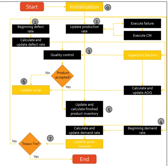
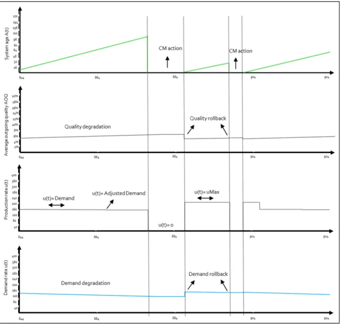
Figure 2.5 Implementation logic chart of the joint control policy of production and quality .36 Figure 2.6 Evolution of system age, AOQ, production rate and demand rate during the simulation run ...39
Figure 2.7 Pareto chart of standardized effects ...41
Figure 2.8 Estimated respond surface contours ...42
Figure 2.9 Evolution of the simulation run in periodic time bases ...46
Figure 2.10 Pareto chart of the second case on ...48
Figure 3.1 Manufacturing system subject to degradation, responsive demand and prevantive maintenance ...57
Figure 3.2 Implementation logic chart of the integrated control policy in case one. ...65
Figure 3.3 Evolution of system during simulation run in case one ...68
Figure 3.4 Standardized Pareto chart for Average net revenue ...72
Figure 3.5 Contours of the estimated response area ...73
Figure 3.7 Evolution of factors during simulation run in case two ...79 Figure 3.8 Standardized Pareto chart for Average net revenue ...82 Figure 3.9 Contours of the estimated response area in case- ...83
LIST OF THE ABBREVIATIONS
At Age of the system during time
λ Demand sensitivity metric Cnq Cost of no quality
Cs Cost of shortage
Ch Cost of inventory
Cinsp Cost of inspection
Crep Cost of repair
Cret Cost of return
𝑥 Finished product inventory level Z Finished product inventory threshold F Proportion of inspection
Mk PM threshold in produced number of parts
Pk PM threshold in decreased price
Pri Price
Pt Proportion of defectives
P0 Quality level of system in its “as new” condition
ANR Average net revenue
Umax Maximum production rate
Ut Production rate
Uins Inspection rate
D Demand rate
D0 Initial demand rate
MTTF Mean time to failure MTTR Mean time to repair
INTRODUCTION
These days, manufacturing companies are experiencing real changes that have a significant impact on their competitiveness, investment and improved production capacity. In the era of communication and information revolution, social media and other means of technology are making clients more aware of product features, which would result to less loyalty and more responsiveness toward product and service quality. Since the new generation of clients such as baby boomers and generation X are far sensitive than their predecessor, manufacturers are expected to face considerable challenges in quality, managing the production and maintenance of increasingly complex manufacturing systems. In fact, the frequency of breakdowns continues to increase over time, disrupting production activities and thus directly influencing the ability of businesses to respond to customer demand that is not constant anymore.
In order to adapt to the varying demand of consumers, manufacturing companies must be flexible and responsive. In an increasingly competitive economic environment, financial issues are crucial. The selling price of the products, which depends on the cost of manufacture, remains very much influenced by the competition. To remain competitive and above all to guarantee a suitable profit margin on the sale of products, the main objective of manufacturing companies is to maintain their product demand in its feasible level.
The existence of varying and dependent demand for product quality requires the establishment of a good quality control policy. This requires rigorous maintenance of production equipment, proper product quality control and production planning that takes into account hazards and good inventory management. In this work, we will address the issues of production management and quality control by asking the following main question:
In the existence of responsive demand, how could we predict and manage non-quality costs and quality control investments in a way to maximize corporate benefits?
• What quality control policy should be implemented? • What production control policy should be implemented? • What repair and maintenance policy should be considered?
All these aspects will be studied in this thesis to maximize the average net revenue.
Given the importance of production planning and quality control for companies, several authors have studied the subject. one of the closest efforts to this study is done by Bouslah, Gharbi et al. (2016) who have developed a new joint approach to production policy, continuous quality control, and a preventive maintenance policy, in order to minimize costs.
The approach used in this thesis for quality control is done by controlling a fraction of the production. In other words, the operator will control each time just a percentage of the parts produced. This approach is suitable for companies that have a continuous production system. The objective will initially be to find a production policy that takes into account outages and that will determine the rate of production depending on the stock, and then find the percentage of products to control.
This thesis is organized into three chapters. The first chapter is a review of literature that introduces some theoretical notions that will be addressed in this thesis and allows us to position our work in relation to others. In the second chapter, we will propose a production and quality control policy with a simulation approach, experimental designs and response surface methodology. In this chapter, we will discuss two cases. In the first case, we will consider a quality control policy with a fraction of continuous sampling and in next two cases, we will verify its efficiency with two other cases, 100% sampling plan, and no sampling plan measurements. The second case is an evolved version of production and quality control policy with a simulation approach, experimental designs and response surface methodology, which considers a delay in demand response based on an average in AOQ. In chapter 3, the system will be studied in the existence of preventive maintenance policy in order to increase the availability of the system and have less amount of costs, resulting from unavailability. In the
second case of this chapter, we propose a policy of production, quality control and corrective maintenance for an unreliable production system with a variable price offer to the demand so as to get a more realistic sense of M1P1 supply chain in real-life. Finally, a general discussion of the study along with a conclusion of the thesis and some future work perspectives is provided at the end of the chapter 3.
CHAPITRE 1 LITRATURE REVIEW
1.1 Introduction
In this chapter, we will first focus on the structure of production systems by presenting the particular case of unreliable systems. Then we will present the critical threshold policy, statistical quality control techniques, and the simulation-based approach to solve such problems. After explaining some applications of prospect theory in related contexts, we will then carry out a critical review of the literature in relation to our subject and will position our work in relation to previous research. After having presented the research question addressed in our study, we will elucidate the objective of our research work. Finally the selected methodology to solve the problem will be presented before concluding.
1.2 Structure of unreliable production systems
In order to understand the structure of unreliable production systems, it is important to define certain terms and concepts in advance.
1.2.1 Production system components in a supply chain context
The so-called "supply chain" is a supply chain made up of suppliers, manufacturers and distributors whose objective is to allow the flow of information, financial resources and products from the ordering of raw materials to the supplier up to the delivery of finished products to the customer (Nakhla 2006).
Accordingly, studied production system involves three main actors: the supplier, the manufacturer and the client. In the context of our work, we will only focus on last two, which are, the manufacturer and the customer, assuming that the supply of raw material is always available.
1.2.2 Production system concepts
In the manufacturing domain, a production system is a set of material resources (production assets) and human resources (managers, managers, operators) aiming to transform the raw material into finished products that satisfy customer requirements. These resources interact with each other through physical flows (products) and information flows (quantity, quality, production plan) (Benedetti 2002). Several criteria are used to classify manufacturing enterprises according to their mode of operation. We can name three main type of classification of production units, in particular, according to the volume of production, the policy of management of production and the nature of production.
I. Production volume
According to this categorizing criterion, (Hounshell 1985)manufacturing companies are classified into three categories of unit production, batch production and mass production enterprises. (Sethi, Zhang et al. 1997)
II. Production Management Policy
There are three (3) modes of production management (Nodem and Inès 2009) either build to stock production, where the management is in push flows, or on-demand production, where the management is done in pull flows or production of hybrid nature as the third type. In push production, production planning is based on forecasts of customer demand; we produce, even if the client is not clearly identified. The pull management policy has been used in the work of Hajji, Gharbi et al. (2011), Lavoie, Gharbi et al. (2010). In other words, their implemented production management policy has been based on an specific customer demand.
III. Nature of production
According to this criterion, we can distinguish three sorts of production starting with continuous flow production systems (for instance metal production, refinery), batch flow systems where products in the form of separate parts are manufactured (automotive industry) (Elhafsi and Bai 1996). Based on this categorizing logic, there are also hybrid systems where both types of continuous and discrete flows are used simultaneously (Bhattacharya and Coleman 1994) .
1.2.3 Process variation factors affecting production system
According to Benedetti (2002), production events are of two types (External and Internal). External process variations are those that do not depend on the company itself. Among these external process variations, we can consider the variation of delivery times of suppliers, the uncertainty of the quality of raw materials delivered by the supplier, the fluctuation of customer demand.
Internal process variations are those that appear within the company and always manages have no power of avoiding them. Among these internal process variations, we can consider machine failures as well as their repairs, the quality of manufactured products that must have a minimum tolerable threshold before being accepted by the customer. Minimum quality is one of the important constraints that allows retaining the customer of a company in addition to adhering minimum order quantity, the delivery time, the place of delivery and the cost of sale (Benedetti 2002).
1.2.4 System degradation
The modeling of quality and reliability degradation in manufacturing systems is a key element that determines to what extent one can imitate the reality of the complex dynamics of these systems, but also to what extent the policies developed with such modeling could be put into practice. In the literature, almost all production control, quality, and maintenance integration models are based on a number of simplistic and unrealistic assumptions in modeling of
manufacturing system degradations. In this section, some important aspects of quality and reliability degradation are discussed that have been demonstrated from several real-life case studies, thought they have been overlooked in the literature.
1.2.4.1 Modeling of quality degradation
Quality degradation is an inherent phenomenon of manufacturing systems. The most widely used mode of quality degradation in the literature is that of describing the production process by two states: the 'under-control' state at the beginning of each new production cycle where all manufactured products conform , and the 'out-of-control' state from the moment the process starts generating nonconforming products. The transition from the 'under-control' state to the 'out-of-control' state is assumed to be random, often following an exponential distribution for reasons of simplification of the modeling(Bouslah, Gharbi et al. 2014).
Rosenblatt and Lee (1986) are among the first researchers to study different forms of quality degradation in production planning. These authors proposed four modes of degradation when the system gets out-of-control, namely:
1. production of a constant proportion of non-compliant products (no degradation) 2. linear degradation of quality over time
3. exponential degradation of quality over time
4. Multi-level degradation of quality with a random transition from one level to another higher level.
This study, which determines the impact of these different modes of quality degradation on the Economic Quantity of Production, has been the subject of several extensions in the literature. Yet most of these extensions are based on Rosenblatt and Lee (1986) first model, which ignores the dynamic aspect of quality degradation. However, there are some exceptions as below: Khouja and Mehrez (1994) considered that the rate of production is flexible and it can affect the intensity of quality degradation (transition from 'under control' to 'out of control'). In fact, this hypothesis is based on several industrial studies that have shown the acceleration of the production rate increases the degradation of quality. For instance, in the case of robotic assembly systems, Offodile and Ugwu (1991) have shown that increasing the speed of
movement of a robot's joining arm results in a decrease in repeatability. Repeatability is defined by the robot's ability to return to the same target point at the beginning of each assembly cycle. This measure is criticized in terms of product quality: Albertson (1983) and Mehrez and Felix Offodile (1994) have shown that degradation of repeatability leads to an increase in the percentage of non-compliant items produced by the robot. The direct effect of the production rate on product quality has also been observed in other industrial contexts such as in the automotive industry and in the machining and cutting processes of metals(Owen and Blumenfeld 2008). Although the effect of the production rate on the intensity of quality degradation has been demonstrated in several industrial studies, the majority of integration models in the literature have completely neglected this type of dependence.
1.2.4.2 Modeling of reliability degradation
In the literature, the reliability degradation a machine is defined to either be dependent on production operations (that is, depending on the use of machine) or time dependent (regardless of the use of machine). Hence, machine breakdowns have often been classified into two categories:
1. Operational breakdowns: Failure of this type can occur only when the machine is operational. The breakdown usually occurs because of machine wear, which depends on the production rate, the production volume during a given cycle or the number of production cycles.
2. Time-dependent breakdowns: Failure of this type can occur even during periods of forced machine shutdown (locked or unpowered machine). The failure rate increases with the advancement of time and is due to phenomena other than wear.
In a thorough industrial study of production line shutdowns in the automotive industry by Buzacott and Hanifin (1978) (Chrysler Corporation case), it is demonstrated that 84% of outages are operation dependent and only 16% of outages are time dependent. Thus, according to the study mentioned above, it is more realistic to use operation-dependent failure models to model the reliability of production systems, since these failures occur much more frequently
in practice than time-dependent failures. Yet, most integrated operations management models in the literature use time-dependent failure models for simplification purposes.
In fact, it is much more complex to model the operational-dependent failures than the time-dependent ones as in the first type of breakdowns, it is necessary to count, in particular, only the times when the machine is operational in the modeling of reliability degradation(Matta and Simone 2016). In a comparative analysis of the two failure models, Mourani, Hennequin et al. (2007) have shown that modeling a machine subject to outages dependent on operations in a production line by a time-dependent failure model can lead to significant underestimation of overall production capacity (up to more than 16% in some cases).
1.2.5 Category of the studied system
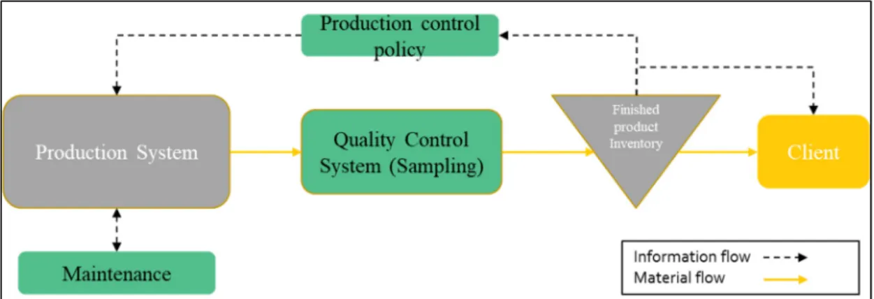
This research project considers a pull and batch production system, that is, firms whose production policy is dependent on customer quality dependent demand as shown in Figure 1.1. We have an unreliable production system that is subject to breakdowns and random repairs and produces non-compliant parts. The possibility of defectiveness (non-compliant production) is depended on the age of production system and continuous until next breakdown event. An inspection policy is put in place to reduce the rate of non-compliant products after production.
The system above proceeds with only one type of finished products. To meet customer demand, the system produces with a variable production rate. The behavior of the system is described by a continuous variable (finished product inventory) and a discrete component (status of machine, on, off).To carry out this work, we will consider the following hypotheses that are commonly used in the literature:
• The machine is subject to breakdowns and random repairs.
• The mean time of malfunction (MTTF) and the average time of repair (MTTR) of the machine are constant and known.
• The different costs are constant and known.
• The demand rate for finished products is quality dependent and decreases from its initial as long as age of machine raises.
• Demand rate restores to its initial value when machine is repaired. • The maximum production rate of the machine is known.
1.3 Critical threshold control policy
Introduced for the first time by Kimemia and Gershwin (1983), the critical threshold control policy is to maintain a security stock of the finished product inventory at an optimal level called a critical threshold. This stock is maintained during production periods to prevent potential hazards that could occur (production system failure, scheduled shutdown). They modeled the control problem using dynamic and stochastic programming, a heuristic allowed them to
approximate the critical threshold that minimizes the total cost of inventory and out of stock. Akella and Kumar (1986) found an analytical solution to the Hamilton-Jacobi-Bellman equations for a control problem of a single machine and a product type, according to breakdowns and random repairs. They have determined the optimal critical threshold which is called hedging point that minimizes the total cost. This control policy has been formulated as follows: 𝑢 = 𝑢 𝑖𝑓 𝑥 𝐷 𝑖𝑓 𝑥 0 𝑜𝑡ℎ𝑒𝑟𝑤𝑖𝑠𝑒 (1.1)
Knowing that 𝑢 is the rate of production depending on the stock and mode of the machine if status variable=1 the machine is in operation, status variable = 0 if the machine is down. For considering preventive maintenance mode of operation, status variable=2. This condition will be studied in chapter 3.
This policy has been confirmed by Bielecki and Kumar (1988). It allows controlling the rate of production according to the instantaneous state of the inventory. When 𝑥 is below the critical threshold z, the rate of production is maximum, when the level of inventory is maintained at the level of the critical threshold it is equal to the rate of the demand. If the level is above the critical threshold, production stops to avoid additional inventory costs.
1.4 Quality control
In order to satisfy the quality demanded by customers, companies are obliged to inspect (control) the products manufactured before delivery to the customer. At the end of the inspection or control, the manufactured products can be qualified as compliant when they meet previously defined specifications, otherwise they are qualified as non-compliant (Baillargeon 1999). In order to guarantee a good quality of products sent to their customers, manufacturing companies have developed several techniques for controlling or inspecting their production. In
the literature, there are several types of quality control, 100% control and acceptance sampling plans.
1.4.1 Hybrid continuous sampling plan
Continuous sampling plans were introduced by Dodge (1943) to control product quality for continuous production systems. A continuous production system is a system dedicated to producing a very narrow range of standardized high volume sales products. In some companies with a complex production process, it is difficult to perform batch control, such as companies producing electronic equipment such as computers or vehicles (the process is done in an assembly line). The best-known continuous sampling plan in industry is Plan CSP-1; this inspection method is carried out according to the following three steps:
• Step 1
100% inspect consecutively manufactured products and continue until a number of compliant products are obtained. This number is the number of permissions still called the clearing interval.
• 2nd step
Once a consistent number of compliant products have been obtained, the 100% inspection is halted; only a fraction f of randomly taken production is inspected at 100% (0 ≤ f ≤ 1).
• Step 3
At this stage, when a defective product is detected in a sample, then a 100% inspection is immediately applied (Step 1) (Dodge 1943).
Since in our case, sampled defective products do not return to the production line we only consider having a fraction of randomly taken parts from production line. Therefore, resulted average outgoing quality of this hybrid continuous sampling plan will be as following:
1.4.1.1 Average Outgoing Quality (AOQ)
According to Dodge (1943), he considers that during the inspection, the products are rectified and re-introduced in the production process. The total quantity of products available after
production remains unchanged. In our system, we considered that during the inspection, the defective products are not rectified, they are discarded, as it is the case for companies whose rectification is impossible or takes too much time or so cost very expensive.
𝐴𝑂𝑄 = 1 − 𝑓 . 𝑝 1 − (𝑓. 𝑝)
(1.2)
According to the formula above, by removing sampled defectives from the system, remaining un-sampled defective parts ((1 − 𝑓). 𝑝) are divided on total remained manufactured parts in order to calculate a precise percentage of remaining defectiveness which is called AOQ.
1.5 Preventive maintenance policy
In manufacturing context, all equipment under production process will get out of service. These events without any preparation or expectation occur sometimes at their worst possible time. In order to control effects of such undesired moments, companies implement preventive maintenance policies in order to minimize Mean Time Between Failures (MTBF) and maximise Mean Time to Failure (MTTF) (Gross 2002).
Considering only Corrective Maintenance (CM) in order to restore machine status after each break down, in chapter 2 and 3 of this thesis, the time of machine breakdown is submitted to an exponential distribution which is subjected to average age of machine as its mean. When machine breaks down, a corrective maintenance action will be proceeded, restoring machine status to the condition, which is as good as beginning.
However, there is no preventive maintenance action in first two chapters, in order to have a better realistic approach, in chapter 3 machine failures are subjected to the cumulative number of manufactured parts since the latest maintenance. Cumulative number of manufactured parts is referred as `virtual age` of machine in the literature. We account break down of machine follows two-parameter Weibull distribution (EL CADI, Gharbi et al. 2017). By using virtual age as break down estimator, preventive maintenance actions can be determined based on threshold consideration in number of cumulative manufactured parts (virtual age). In this manner, PM actions will occur after passing `MAge` threshold, turning system status to PM mode.
1.6 Prospect theory
Individuals choosing behaviours under risk is not consistently explainable with the assumptions of utility theory in a persuasive manner. In general, people weight outcomes below their exact value that come from probability-outcome compared by outcomes, obtained with 100% certainty. Such type of tendency, which is defined as the certainty effect, leads to risk aversion behaviour in choices with 100% gains to risk seeking behaviour in choices with 100% losses (Kahneman and Tversky 2013). In other words, when people face in gain opportunities, prefer to choose certain options rather than any other probable choice (which may have more gain but equal utility). In reverse, in case of loosing, people try to go for options with more uncertainty to maybe avoid expected losses.
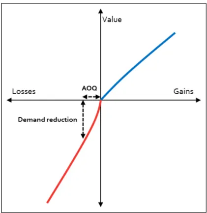
The value function as presented in figure 1.2, has the shape of concave in gain area however, in loss area due to loss averse behaviour explanation, it has became steeper (Tversky and Kahneman 1992). Illustrating that people are afraid of losing far more than joy of winning.
Figure 1.2 A hypothetical value function (Tversky and Kahneman 1992)
In addition, there is a tendency in this theory called isolation. According to isolation effect, individuals have a tendency toward discarding of some shared components of a prospect under their considerations. Isolation effect will lead individual to have changeable preferences facing with the same choice, presented in other ways (Kahneman and Tversky 2013).
Kahneman (1979) also has illustrated another aspect of individual decision making by a probability scale which is nonlinear and explains its transformation by overweighting small probabilities and moderating/ underweighting high probabilities. In other words, the probability weighting function shows that individuals do not respond to probabilities in a linear manner and this is proven by the study of Gonzalez and Wu (1999).
The weighting function proposed by Kahneman (1979) was not defined near the end points however it has shown underweighting of large scale probabilities (Gonzalez and Wu 1999) and overweighting of small ones. For instance, according ECONOMIST, there is a very small risk of die in an aircraft crash less than 1 in 5.4 million. Accordingly, this little possibility is big enough for passengers to purchase travel insurance, showing how considerably this risk is
overweighed for individuals. This approach is widely used by gambling and insurance industry during centuries (Kahneman and Tversky 2013).
In above figure, the probability weighting function is denoted by π (p), this function maps the interval of 0 and 1 onto itself. Tversky and Kahneman (1992) then developed above weighting function as they believed that changes in probability appear more dramatic in the neighborhood of end points rather than middle. This reversed S shape got later proved by empirical studies (Gonzalez and Wu 1999).
According to prospect theory, an alternative theory of choice has ben developing during last 40 years by assigning values to gains and losses rather than simply defined final assets. Decision weights are replaced with probabilities of utility theory to better address behaviour of individuals.
1.6.1 Prospect theory applications
During recent years, applications of standard microeconomics tools in order to have precise assumptions of human behavior which is imported from psychology has begun and vastly developed which according to Rabin (2002), this has shaped `second-wave behavioral economics` (Rosenkranz and Schmitz 2007). In this regard, one of the most prominent economic paradigms, which has helped to comprehend reference-based behavior of people in utility, is prospect theory (Rosenkranz and Schmitz 2007). In general, applications of prospect theory could be segmented in 3 major, general groups as below:
1.6.1.1 Reference points
Based on prospect theory, reference point is a measure of outcome perception by people. People verify utilities by comparing with reference points(Kahneman 1979). It is to say that factors who determine the reference point are not specified in the context (Werner and Zank 2019). This point acts as a boundary to distinguish gains and losses from each other(Tversky and Kahneman 1992).
Among recent publications, reference point is vastly utilized in major subjects such as pricing in the studies of Hsieh and Dye (2017) for optimal dynamic approaches by considering reference price as a basis of comparison for customers deepening on their degree of remembrance. Also in finance, reference point is considered as the risk-free rate and in insurance industry is referred to expectations of future outcomes (Barberis 2013).
1.6.1.2 Risk aversion/seeking
As mentioned in figure above, people has risk aversion attitudes in gain occasions though in loss occasions they prefer to be risk-seeking(Kahneman 1979). This type of behavior has been studied in terms of extend of gains, implying that people tend to take risks of smaller monetary gains rather than big ones (Weber and Chapman 2005) or the fact that risk aversion has a rising tendency between infancy and adulthood (Levin and Hart 2003).
According to Kahneman (1979), individuals are not particularly risk averse or seeking in every situation that incorporate two different functions in mentioned loss and gain areas. This inconstant type of respond has been taken into account in demand studies during recent years. Research in mid 90s illustrates that tolerance of risk changes among different groups of individuals (Sewell 2009). For instance, the cluster of high educated, rich, drinkers, people with no insurance immigrants, Jewish individuals and races such as Asians are risk seekers while the second cluster, comprising of average wealth and source of income, those with health insurance and middle education level plus people who are in their sixties is risk averse (Barsky, Juster et al. 1997).
Accordingly, Hsieh and Dye (2017) has considered three different comportments of customer demand based on prospect theory assumptions. Their aim of study was to propose an optimal dynamic pricing policy for a demand with three different characteristics (following prospect theory assumptions) in relation with stock inventory, selling price and deterioration. According this study, penetration strategy is suitable in the case that reference price is lower than market (case of risk seeking demand type) and skimming strategy best suits for risk averse type of demand behavior.
Assuming risk averse attitudes in times of loss and risk seeking one in comparison with the reference point, Swinyard and Whitlark (1994) has applied customer satisfaction and dissatisfaction in store return intentions. Proving findings of prospect theory, they found that dissatisfaction affects two times more store returns intentions than satisfaction.
Briefly and based on our best of knowledge, risk averse approach in times of loss has generally used in majority of reviewed research.
1.7 Problem Statement
To the best of our knowledge, according to the law of demand, customer demand of certain commodity has always been assumed to be directly affected by price, in the context of demand and supply (Marshall 1892). This sort of inverse relationship between price and demand can be affected by other factors such as quality improvement or degradation, considering shift of demand curve. In other words, accordingly, demand curve shifts may be caused by a variety
of reasons such as income raise of customers, unexpected changes in product’s quality, its substitutes or complements (Marshall 1892). On the other hand, utility is another factor that deals with levels of demand. Utility is the degree of satisfaction in costumers by committing an actions in decision making, individuals tend to increase their utilities (Kapteyn 1985). Higher levels of utility curves imply better provided satisfaction for customers, however these are not clearly explainable without consumer behavior theories(Kapteyn 1985).
Since better quality in product could be referred to better satisfaction and higher utilities, there is no specific function introduced in economics and marketing literature to estimate demand degree of response to improvement/degradation in quality. Even by assuming the fact that the non-quality amounts affects the demand in a negative way, the extend of this response needs to be well- addressed in a way to conform to known demand dynamics. This study is a strive to find a proper direct deal between quality measurements in quality dependent demand with the use of prospect theory for demand response measurement. In this work, the amount of demand response to any non-quality will be determined and an integrated policy for a production system with quality and reliability degradation needs to be defined, optimizing its average net revenue.
1.8 Research objectives
The main objective of this research is to implement a proper production control, maintenance and pricing policy while there is responsive demand comportment toward non-quality output of the system. Therefore, to reach the main objective above, following sub-objectives are considered as well:
1. To maximize total profit function rather than minimizing total cost of production regarding to the context of study in demand area.
2. To adequately model the complex dynamics of product quality degradation and machine reliability like real manufacturing systems. This involves modeling dependency relationships between quality and reliability degradation, machine aging, and production rate.
3. To develop a new approach to design sampling plans in the context of integration with production and preventive maintenance policies.
The objectives above are based on five main assumptions to be validated as part of this study, below:
1. It is possible to use sampling plans for production systems with a degradation of quality by ensuring the fulfillment of imposed requirements on after-control quality(Bouslah, Gharbi et al. 2018).
2. The level of final quality after-control is the result of the configuration of all the parameters of production control, quality and maintenance of the manufacturing system. In other words, the level of quality, perceived by client does not depend only on the quality control parameters(Lavoie, Gharbi et al. 2010).
3. Demand of client reacts to the level of perceived level of final quality after control and this behavior is considered to be loss-averse according to prospect theory.
4. There is no rectification plan estimated in quality control part of system. All inspected defectives items get out of the production process(Hajji, Gharbi et al. 2011).
5. Any delivered defectives items to clients will be collected and taken out of production system with no rectification (EL CADI, Gharbi et al. 2017).
1.9 Thesis’s structure
The research work carried out as part of this thesis in the form of two scientific articles. These two articles are presented in chapters 2 and 3.
In article one, which is presented in chapter 2, responsive demand comportment in the existence of quality and production control systems is taken into consideration. This article has contributed to two types of responsive demand behavior, instant and delayed when degradation and maintenance policies are implemented based on real-time units and exponential distribution for the reliability of the production system.
The second article is about the intervention of preventive maintenance policies into the relationship of responsive demand and production system, considered in article one. The
approach is to increase net corporate revenue in the existence of operation caused failures of the production system based on an accumulated number of production. Later, this article considers pricing policies in the context of competition to reflect a better image of reality by use of prospect theory assumptions, this time in price, quality and demand relationship.
1.10 Research methodology
The adopted approach in this study has been about modeling and solving problems of joint design and optimization of some integrated models, proposed in two articles. These steps are summarized by the following methodology:
1. Definition of the objective and assumptions of the problem under study: This step consists of understanding the problematics and objectives of the study and modeling of determined assumptions.
2. Mathematical formulation of the problem under study: This step is about identifying decision variables and formulating the objective function along with the constraints of the problem.
3. Using a simulation-based optimization approach: This step consists of two sub-steps: The first is to develop and validate a simulation model with the ARENA software, based on the analytical modeling of the problem. Next, to use simulation-based optimization techniques, such as Response Surface Methodology, meta-heuristics, and gradient-based search methods to determine the optimal solution.
CHAPITRE 2
The policy of joint quality and production control for an unreliable manufacturing system subject to quality-dependent demand
2.1 Abstract
In this chapter, a joint production control policy comprising of quality and production decision variables has been developed for unreliable production units with an age-based quality degradation and a quality-dependent demand, which responds to the quality levels of delivered products. Using hedging point policy that uses a certain amount of stock in the finished product inventory, the production rate of the machine gets controlled to avoid the excessive cost of shortages during the stop time of production such as maintenance and breakdown and change in demand amounts. The principal objective of this study is to maximize the total profit of the manufacturing system by setting a certain amount of safety stock quantity and a fraction of production output as the sampling of the quality control. By using response surface methodology based on gathered results of the simulation, a simulation-optimization approach for the developed stochastic mathematical model is developed. Results of the study clearly show some very strong ties between safety stock levels and percentage of sampling as the decision variables. This confirms the need for jointly and simultaneously application of policies in this integrated model. Altogether, a joint production and quality control policy in the presence of quality-dependent demand is proposed. Moreover, it is illustrated that setting periods during the machine’s available times for computing average outgoing quality and getting demand reactions, will result in more total profits, comparing with the initial assumption.
2.2 Introduction
In today’s world, enterprises are paying more and more attention to their product’s quality through their supply chain to increase their customer satisfaction which literally results into higher demand (Modak, Panda et al. 2015). Except for quality consideration, demand satisfaction in today’s modern world really matters and the consequences of unsatisfied demand such as losing market share, brand and reputation damage, loss of sales and service level reduction are really significant (Jabbarzadeh, Fahimnia et al. 2017). Although demand and quality are getting closer, over past years of manufacturing and quality studies there have been three approaches towards demand.
2.2.1 Constant demand approach
In the first group, it is assumed to have a constant rate of demand under certain circumstances. For instance, Hlioui, Gharbi et al. (2015) have considered the demand rate stable and constant factor and they proposed a hybrid policy which always outperforms the 100% screening or discarding policies. In another work by Hlioui, Gharbi et al. (2017) in the same context of manufacturing and quality control, a dynamic supplier selection policy has been proposed, assuming the demand rate is unchanged in all time. Again, This assumption has been used in the work of Bouslah, Gharbi et al. (2018) in the case of finding a policy, covering production, quality, and maintenance control in a set of two machines which the reliability of the second machine is affected by the output of the first machine. The quality management system has been generally considered as an element of motivating and penalizing suppliers in the study of Starbird (2001) in an inspection policy to deliver better products based on determined quality targets of customer. However, in this study demand is deterministic and remains unchanged. To the best of our knowledge, in such simultaneous production and quality control policy design during recent years, there has not been any other demand assumption but constant and continuous.
2.2.2 Demand uncertainty approach
In the second approach, which is generally popular in the supply chain network, demand uncertainty is due to the existence of some factors. Callarman and Hamrin (1984) have examined tree different lot sizing rules in the presence of stochastic demand. Another study which considers market demand as a random variable and a probability density function (PDF) for this is done by Mukhopadhyay and Ma (2009) to address quality and demand uncertainties in production and procurement decision making. Generally, a stochastic behavior has been taken into account this behavior as Van Donselaar, Van Den Nieuwenhof et al. (2000) used a uniform distribution in a simulation-based experiment design to verify how wrong demand assumptions could affect supply chain planning. This study has analyzed the case of a truck manufacturer in the Netherlands and used its historical demand data. One year later, Caridi and Cigolini (2001) have proposed a buffering strategy to control uncertainty of market demand, using safety stock. Their main objective was to make corporate able to monitor in real-time the amount of demands however, this study does not support any mathematical model for demand behavior.
2.2.3 Dependent demand approach
In the third approach, despite the assumptions of mentioned production and quality based works, nowadays, customers are engaged with those products, offering better quality at a reasonable price and business demand which is derived from individual demand is, even more, fluctuating (Armstrong, Adam et al. 2014). Gurnani and Erkoc (2008) have taken into account a decentralized distribution channel of manufacturer and retailer, considering a level of quality that is chosen by the manufacturer and particularly, this quality level determines the product demand along with selling efforts that are chosen by retailer. Supposing that quality and price specifications delivered by suppliers directly affect potential market demand. Yu and Ma (2013) have studied demand behavior affected by the pricing of the manufacturer and direct delivered quality of the suppliers in an optimal decision sequence with three different scenarios. In this study, all three decisions models with separated decision sequences are implemented to maximize the profit of each player (manufacturer, supplier). In a closed-loop
supply chain framework, Maiti and Giri (2015) have assumed to have a quality and price dependent demand for two completely different manufacturing and remanufacturing process lines. The supply chain in this study includes a manufacturer, retailer and third party for remanufacturing process. In other contexts rather than above, quality responsive demand has been studied enough. In the study of Modak, Panda et al. (2015), the demand of retailer is related to three factors of quality, selling price and warranty by considering profit function optimization for both manufacturer and retailer in the context of two layers supply chain. According to this interactive relationship which is modeled using Stackelberg game, the retailer is focused on maximizing its margin based on provided price, quality and warranty while the wholesale price of goods of the manufacturer is depended to its produced level of quality, however, demand and quality factors are assumed to be following stochastic behavior. Swinyard and Whitlark (1994) have used prospect theory with the idea that dissatisfaction of customers results more in their store return intentions than their satisfaction. Accordingly, customers who were dissatisfied tended to not be back two times less than those satisfied customers who were willing to be back.
Following prospect theory application in demand area, some studies have worked on framing effect as a tendency to avoid any risk when people face with positive options with exact gain and to be risk seeker when a negative option is presented beside exact loss (Kahneman 1979). In other words, Tversky and Kahneman (1981) have explained that the attractiveness of choices to choose, changes when the decision problem gets framed in other manners. According to this, Wu and Cheng (2011) have verified the impact of framing bias on decision-making attitude of internet buyers to see how information presentation stimulate demand of online customers with different product knowledge. In a nutshell, the current study has aimed the third approach, using prospect theory applications to well address demand responses in the context of manufacturing and quality consideration which is the case of first explained approach.
2.3 Problem statement
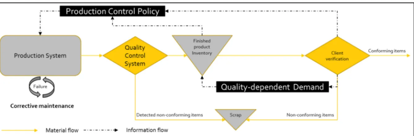
Considering an imperfect production unit, illustrated in figure 2.1, operating under a stochastic type of failures and repairs throughout its operation. This unavailability usually leads to having interruptions during the production process, resulting in shortages in satisfying demand rate and lost sales. Failure incidents will be repaired by implementing corrective maintenance measurements and bring back the system status to its initial condition (as good as new) with minimum defectiveness possibility since such actions normally are about replacements of broken components in a real context (Bouslah, Gharbi et al. 2018). The amount of time spent on corrective maintenance follows a random distribution. In addition, the production system is subject to aging which results in degradation of the quality in the percentage of manufactured products. As long as the machine is not broken and its age is raising, degradation of quality increases in the proportion of defectiveness until a predefined maximum limit, set to prevent having negative values of demand in responding to the quality level. Quality and reliability degradation of the intended production system is not dependent to its operation scale however, this manufacturing system produces with a flexible rate between 0 and maximum production capacity. Such production line feeds a quality-dependent demand, which decreases its rate upon receiving defective items by measuring the proportion of delivered no quality products. Because of mentioned demand dynamics dealing with quality, a quality control policy is designed to conduct a continuous checking over a portion of production output 0 ≪ 𝑓 ≪ 1 and remove out of range items as scrap. Production line does not rectify non-conforming parts, after quality control inspection. Unsatisfied demands in terms of quantity will not be back-ordered and all remaining no-quality items, passed to the customer will be returned and scraped with a rejection cost. Raw material stream in this study is considered to be constant and infinite to satisfy the production unit. The objective is to maximize the total net revenue function, comprising of average gross revenue, the average cost of inventory and shortage, the average cost of inspections, the average cost of CM and the average cost of no-quality product returns.
2.3.1 Degradation model
The production unit status is described by two different variables. The first variable is a discrete-state for showing the operational condition of the production unit at time t. This discrete variable (𝑠(𝑡)) takes only two values 0,1 . In other words, if 𝑠(𝑡) = 0 it means that the system is out of order and under corrective maintenance. If 𝑠(𝑡) = 1 the system is under operation. The second descriptive variable records systems age from the last corrective maintenance until time t. This variable (𝐴(𝑡)) will determine the age of the production system such that in time of being out of service will keep its latest amount and not increase, following 2.1 equation:
𝜕𝐴(𝑡) 𝜕𝑡 = 0
(2.1)
It is considered that the state variable follows an exponential distribution. Therefore, failure of the production system is not dependent on the extent of the operation and no preventive maintenance is taken into account. Although the reliability of the system has no tie with the scope of operations, quality degradation of the system augments during system’s available time (𝑠(𝑡) = 1). Hence, degradation of quality is defined as increase in the proportion of defectiveness in intended production system. This is calculated, using 2.2 equation:
p(A) = p η 1 − e . (2.2)
Above equation represents the possibility of defectiveness in the production rate. This percentage is dependent on the age of the system. Hence, in order to show degradation, as time goes on, defective percentage augments. P0 is defined as the quality level of the system in its
“as new” condition. It is a very small percentage of defectives items produced by the manufacturing system at its initial state. The sum P0 η determines the peak percentage of defectives items.
Figure 2.2 Quality degradation over time in correlation with the system age
Because demands amounts might face huge drops such as zero or negative without having any control on this factor, the degradation factor is designed in a way that takes a constant amount toward infinity. Figure 2.2 clearly illustrates the effects of changing factors on the shape of drawn functions. It is also assumed that coming raw material into the system is defect-free.
2.3.2 Quality-dependent demand nature
In this study, the possibility of defectiveness has been interpreted as a perceived loss of a customer who treats according to a loss-averse behavior in prospect theory. Based on Tversky and Kahneman (1992) findings, there are two different functions that describe customer
responses. Function f(x) for the explanation of perceived gains and function g(x) for the loss area. f(x) = 𝑥 𝑖𝑓 𝛼 > 0 log(𝑥) 𝑖𝑓 𝛼 = 0 1 − (1 + 𝑥) 𝑖𝑓 𝛼 < 0 (2.3) g(x) = −(−𝑥) 𝑖𝑓 𝛽 > 0 − log(−𝑥) 𝑖𝑓 𝛽 = 0 (1 − 𝑥) − 1 𝑖𝑓 𝛽 < 0 (2.4)
As mentioned, the possibility of defectiveness is accounted for a loss for people. Therefore, following findings of Tversky and Kahneman (1992), function g(x) will build the response of demand to such existing imperfection. To have precise values of 𝛽, the empirical results of Tversky and Kahneman (1992) are used as our benchmark the quality-dependent demand is built in equation 2.5 as below:
𝐷 = 𝐷 (1 − 𝜆 ∗ 𝐴𝑂𝑄 ) (2.5)
Where 𝛽 is benchmarked as 0.88 and 𝜆 is equal to 2.25 that show customer sensitivity and scale of response to any received percentage of defectiveness that refers to average outgoing quality (AOQ) explained in section 1.4.1.1.
Briefly, the above demand function determines the extent of the customer response to any detected level of defects, delivered to the customer as average outgoing quality. Upon having AOQ level, demand function decreases its initial rate of 𝐷 to a less rate, affected by the power of 𝛽 and multiplied by𝜆.
Figure 2.3 Demand function
In other words, demand function penalizes any scale of non-quality by reducing its determined rate even more than the exact amount of defects.
2.3.3 Production policies
The efficient mean of performing production policy is known as the production rate (𝑢(𝐴)) of this unreliable manufacturing system which is constrained between its zero and maximum capacity (0 ≤ 𝑢(𝐴) ≤ 𝑈 ). As one of the most well-known production policies for continuous flow and unreliable systems is presented by Akella and Kumar (1986), we use this hedging point policy (HPP) in order to reach to an efficient rate of production subject to system availability and inventory levels.
𝑢 =
𝑢 𝑖𝑓 𝑥 < 𝑧 𝑎𝑛𝑑 𝑠(𝑡) = 1 𝐷 𝑖𝑓 𝑥 = 𝑧 𝑎𝑛𝑑 𝑠(𝑡) = 1 0 𝑜𝑡ℎ𝑒𝑟𝑤𝑖𝑠𝑒
The dynamic of mentioned HPP policy is illustrated in equation 2.6 such that it sets production rate on its maximum (𝑢 ) when finished product inventory level is less than HPP’s threshold, named z. In case of reaching finished-product inventory level to threshold level of z, the system tries to keep its maximum value of z in inventory levels by choosing to produce as much as the demand rate. According to HPP, the system stops its production in case of having excessive amounts in its finished-product inventory or failure. Due to the presented HPP policy, there are three system phases: the first phase leads the system to produce in its maximum rate to build its safety stock of z. However, such safety stock building is not linear and it depends on the proportion of defectives items, detected by the inspection and failure of the machine which affects such increase toward reaching to maximum z threshold. In the second HPP phase, the system production rate is adjusted to the demand rate in order to keep maximum amounts of safety stock z. It is to say that sometimes second phase doesn’t occur if system faces any failure in phase one because it takes time again to provide the maximum finished-product inventory of z and as system failure comportment is exponential, production policy will take place between phase one and three. In the last phase (three), the system is under reparation due to corrective maintenance. In this period of operation, the system rate is null, facing finished product inventory drop with the rate of demand.
2.3.4 Quality control policies
Explained quality-dependent demand reacts to the fraction of received defective items by reducing its rate. Therefore, it is crucial to avoid facing high percentage of non-quality in delivered orders by verifying an optimized fraction of production as the quality control. Otherwise, high percentage of non-quality in the system this will result in a very low rate of demand.