Concept de corrélation dans l'espace fréquentiel de Fourier pour la télédection passive de la terre : application à la mission SMOS-Next
171
0
0
Texte intégral
Figure
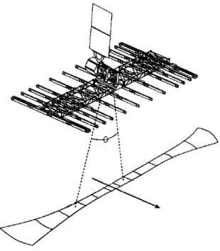
![Figure 1.1: Schematic diagram of a two-element interferometer expressed for an ideal two-element interferometer as [8],](https://thumb-eu.123doks.com/thumbv2/123doknet/2146794.9077/32.918.327.620.96.376/figure-schematic-diagram-element-interferometer-expressed-element-interferometer.webp)
+7
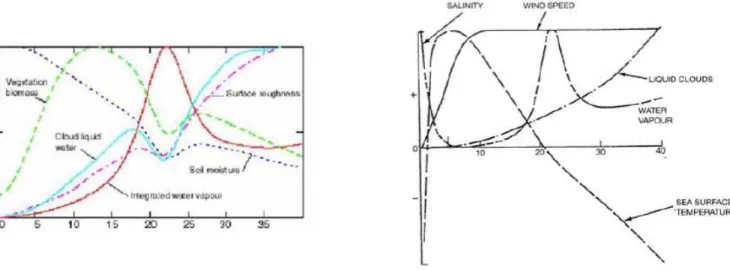
![Figure 1.6: Microwave transmissivity as func- func-tion of increasing biomass [31]](https://thumb-eu.123doks.com/thumbv2/123doknet/2146794.9077/37.918.526.778.110.415/figure-microwave-transmissivity-func-func-tion-increasing-biomass.webp)
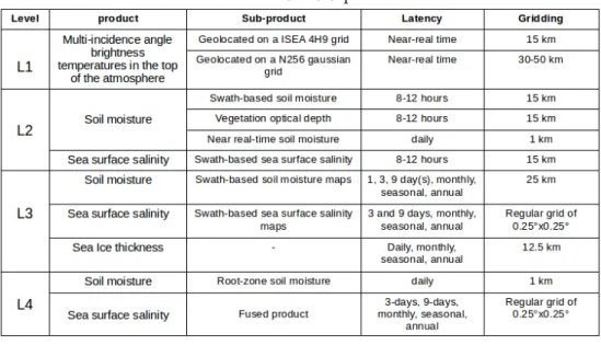
![Table 1.7 depicts the expressed users’ requirements in the specific Earth observation application of the study of coastal zones [68] (see next chapter for more details)](https://thumb-eu.123doks.com/thumbv2/123doknet/2146794.9077/58.918.124.842.119.534/depicts-expressed-requirements-specific-observation-application-coastal-chapter.webp)
Documents relatifs