The two-machine open shop problem with time delays

COMME EXIGENCE PARTIELLE

DE LA MAITRISE EN INFORMATIQUE

OFFERTE À

L'UNIVERSITÉ DU QUEBEC À CHICOUTIMI

PAR

LI CHUAN ZHANG

THE TWO-MACHINE OPEN SHOP PROBLEM

WITH TIME DELAYS

Research on scheduling problems as we know it nowadays dates back to 1950s. Indeed, in 1954, Johnson described an exact algorithm to minimize the overall completion time (known as the makespan) for the two-machine flow shop problem. This resulted in a new discipline of operational research known as scheduling theory.

Scheduling theory deals with the attempt of using a set of scarce resources in accomplishing variegated tasks in order to optimize one or several criteria. The resources and tasks are commonly referred to as machines and jobs, respectively. There is a broad spectrum of definitions for the tasks and resources. For example, the resources can take the form of production lines in workshops, airport runways, school classrooms, etc. Furthermore, the process of fulfilling a task in a given machine is sometimes called an operation. For instance, a task may be represented by the work-pieces processed on production lines, the aircrafts taking off and landing at airports, the teachers lecturing in classrooms and so on. Let us note at this stage that machines and jobs may have been characterized by many other factors such as speed, time of availability, duplication, etc for the former, and precedence constraints, due dates, time lags for the latter. These factors must be taken into consideration when formulating a scheduling strategy if we want to produce a realistic solution.

Generally speaking, scheduling problems fall into the following three categories: A single machine model, parallel machines model and multi-operation model. The models known as multi-operation model are flow-shop, open shop and job shop.

In addition, a scheduling solution is evaluated according to a given criterion or sometimes to a set of given criteria such as the minimization of makespan, mean finish time, number of tardy jobs, etc.

This thesis is mainly concerned with the problems of minimizing the makespan criterion in a two-machine open shop environment with time delay considerations.

In order to better approach the resolution of this problem, some basic concepts on scheduling theory and related knowledge, such as the theory of NP-completeness,

have been introduced. It is important to analyze the advantages and disadvantages of different algorithms, in order to come up with an adequate solution.

We presented in this dissertation the resolution of the two-machine open shop problem with time delays along the following lines. First, we start by looking at special cases to solve to optimality in polynomial time. Then, we move onto the design of heuristic algorithms, based on simple rules. Finally, we discuss two meta-heuristic algorithms and lower bounds, and undertake simulation experiments to analyze their performance in the average case. For heuristic algorithms, we discussed some approaches that evaluate their performance. Regarding the meta-heuristic approach, we used the simulated annealing and the tabu search algorithms, respectively. We then improved the second approach by adding the intensification and diversification strategies. Finally, we proposed a new hybrid approach to solve our original open shop problem in the hope to improve and speed up the quality of the solution.

Acknowledgements

I would like to take this opportunity to acknowledge the people who have helped me with my studies.

First of all, I would like to express my gratitude to my supervisor, Professor Dr. Djamal Rebaine, who provided me generous help with my study, has given me many valuable suggestions and comments on my dissertation, and improved significantly my English, the clarity and the style of my writing.

I also give my greatest appreciation to my family in China. I especially appreciate the consistent support and encouragement my parents and brother have provided to me while at home in China and abroad in Canada.

I would also like to thank my friend Mr. Wei, for proofreading and correcting my dissertation drafts.

Special thanks to my friends who are also studying here and have been accompanying me and offering me educational assistance and support.

CONTENT

SUMMARY II

Acknowledgements IV

CONTENT V

LIST OF TABLES VIII

Chapter 1 General Introduction 9

Chapter 2 Scheduling Problems 12

2.1 Introduction 13

2.2. Scheduling models 13

2.3 Basic Definitions 17

2.4 Three-Field Notation 18

2.5 Gantt Chart 20

2.6 Scheduling with time delays 21

2.7 A Brief introduction to the complexity theory 22

2.8 Analysis of Scheduling Problems 26

2.8.1 Exact methods 27

2.8.2 Relaxation 27

2.8.3 Pseudo-Polynomial Algorithms 28

2.8.4 Approximation Algorithms 28

2.8.4.1 Analytic Approach 29

2.8.4.2 Experimental Approach 30

2.9 Description Of An Exact And A Heuristic Approach 30

2.9.1 Exact Algorithms 30

2.9.2 Heuristic Algorithms 33

2.9.3 Meta-heuristic Algorithms 34

2.9.3.1 Simulated Annealing 35

2.9.3.2 Genetic Algorithms 36

2.9.3.3 Tabu search method 39

Chapter 3_The Two-Machine Open Shop without Time Delays 42

3.1 Introduction 43

3.2 Gonzalez-Sahni Algorithm 43

3.3 Pinedo-Schrage algorithm 45

3.3.1 Experimental study 51

Chapter 4 The Two-Machine Open Shop With Time Delays.... 53

4.1 Introduction 54

4.2 Lower Bounds 55

4.2.1 Unit-time operations 56

4.2.2 General processing times 59

4.3 Heuristic approach 61

4.3.1 Worst-case analysis 62

4.3.2 Experimental study with unit-time operations 63

4.4 Meta-heuristic Algorithms 67

4.4.1 Internal Structure 69

4.4.1.1 Simulated-Annealing 69

1. Basic algorithm 69

2. Improvement experiments 73

4.4.1.2 Tabu search 80

1 Basic algorithm 80

2.1mprovement experiments 84

4.4.2 A Hybrid Algorithm 89

4.4.2.1 Basic idea of the hybrid algorithm 89

4.4.2.2. Experiment Results With The Hybrid Algorithm 91

General Conclusion 93

Rferences 96

LIST OF FIGURES

Figure 2- 1: Single Machine Model 14

Figure 2- 2: Parallel Machine Model 15

Figure 2- 3; Flow Shop Model 15

Figure 2- 4: Open Shop Model 16

Figure 2- 5: Job Shop Model 16

Figure 2- 6: Gantt Chart 20

Figure 2- 7: Relationship between P, NP, NPComplete, NP-Hard classes.... 25

Figure 2- 8: Single Point Crossover 37

Figure 2- 9: Two Point Crossover 38

Figure 2-10: Uniform Crossover 38

Figure 3- 1: Two partial schedules 45

Figure 3- 2: Optimal Solution for GS Algorithm 45

Figure 3- 3: Optimal Solution for LAPT Algorithm 46

Figure 3- 4: Optimal Solution for LAPT Algorithm 47

Figure 3- 5: Optimal Solution for Case 1 48

Figure 3- 6: Optimal Solution for Case 1 48

Figure 3- 7: Optimal Solution for Case 2 49

Figure 3- 8: Optimal Solution for Case 2 50

Figure 3- 9: Optimal Solution for Case 2 50

Figure 3- 10: Optimal Solution for Case 2 51

Figure 4-1: A Schedule for OS1 57

Figure 4-2: Case where p

• < p

60

Figure 4-3: Case where p

> p

61

Figure 4- 4: Algorithm 1 through Example 4-1 65

Figure 4-5: Algorithm 2 through Example 4-1 66

Figure 4-6: solution produced by the Calculation module 72

Figure 4-7: Cooling Factor = 0.01 74

Figure 4-8: Cooling Factor = 0.99 74

LIST OF TABLES

Table 2 - 1 : Instance with m = 2 and n = 3 20

Table 2- 2: Instance with m = 2 and n = 4 21

Table 2- 3: Time Delays in Example 2-2 22

Table 3-1: Processing time for an instance with four jobs 44

Table 3- 2: Effect of Lower Bounds for TS algorithm 52

Table 4 - 1 : Instance with N=9 64

Table 4- 2: Results Found for Algorithm 1 and Algorithm 2 67

Table 4-3: Cooling Factor = 0.8 73

Table 4-4: Cooling Factor = 0.9 75

Table 4-5: Cooling Factor = 0.95 75

Table 4-6: Cooling Factor = 0.99 76

Table 4-7: Intensification Module Added 78

Table 4-8: Diversification Module Added 79

Table 4- 9: Intensification and Diversification Module Added 80

Table 4-10: Results for the Basic Tabu search 83

Table 4-11: Results for the Flexible Tabu search 83

Table 4-12: Initial Sequence for Algorithm 1 85

Table 4-13: Initial sequence for Algorithm 2 85

Table 4-14: Results for Intensification Model 87

Table 4-15: Results for Diversification Model 88

Table 4-16: Results for Intensification and Diversification Model 89

Table 4-17: Results for the Hybrid Algorithm 92

Chapter 1

In modern societies, all walks of life bear witness to progressively fiercer competition. As a result, extensive management mode cannot satisfy the demands posed by the competition anymore. Therefore, the question of how we are able to be more effective and take advantage of resources has become a focus that has captured the attention of all businesses and is becoming one of the core components for modern enterprises and administrations. A scheduling problem is solved by working out an appropriate plan for a set of tasks to be performed over time on a set of scarce resources to achieve one or several goals. Within the task-performing period, a certain power over resources needs to be consumed. However, the number of resources that a person (enterprise, technology) can use is finite. The ultimate goal of solving a scheduling problem is to, on the basis of achieving one or several objectives, ensure (or realize) the highest utilization rate of the resources as much as possible. Generally speaking, a scheduling problem may, according to different processing demands, fall into three categories: A Single Machine Model, Parallel Machines Model and Multi-Operation Model. In most of the articles involving scheduling problems, the problem of serial workshops (flow-shop) has been one of the first to be studied by the early fifties. Johnson, in 1954, was the first to study the problem of flow-shop with two machines [Johnson, 1954]. Then, appeared later studies other multi-operation models such as the job shop problem and the open shop problem (or flexible, depending on the design of the workshop). It has been found, at the early stage of scheduling theory, that there is a huge gap between research findings and practical production problems. The most important problem is the neglect of the inevitable limitations on the practical producing process such as the period between the finishing time of one operation of performing a task and the beginning time of its next operation, denoted as time delays, time lags, communication time delays, or transportation times, depending on the context. Time delays may take different forms in diverse industries. For instance, time delays may refer to transportation times to move a job from one place to another or to the time of heating or cooling a job before another process takes place.

algorithms: the exact approach and the approximation approach. The latter approach can be divided further into heuristic algorithms and meta-heuristic algorithms.

This dissertation is mainly concerned with study of minimizing the overall completion time, also known as the makespan or the schedule length, on two-machine open shop problems with time delays considerations.

In addition to the introductory chapter, this thesis contains four chapters and a conclusion. The second chapter introduces some basic definitions, concepts and scheduling models such as the Gantt chart, time delays, and details on appropriate algorithms to solve scheduling problems.

The third chapter first considers the two-machine open shop problem without time delays which is solved by two exact algorithms: the Gonzalez (GS) algorithm and the Pinedo and Schrage (LAPT) algorithm. For implementation reasons, we proposed a simple way of stating the latter algorithm, along with a proof of its optimality. We also conducted a simulation study to compare the performance of these two algorithms.

The fourth chapter is about the two-machine open shop with time delay considerations. This chapter is divided into two parts. Part 1 mainly presents heuristic algorithms for some special cases. The performance evaluation of the different heuristic algorithms involves the analytic and the empirical approaches. Part 2 introduces meta-heuristic algorithms for the general open shop problem. The strategy of the meta-heuristic algorithms includes stopping criteria, internal structure, and hybrid algorithms. For the stopping criteria, the algorithms are interrupted by some special conditions, such as the makespan is equal to a lower bound. We propose and prove several lower bounds for the problem under study, and apply them to our meta-heuristic algorithms. For the internal structure, the development of a tabu search algorithm and a simulated annealing algorithm is discussed with the addition of intensification and diversification procedures. For the hybrid algorithm that we propose, we combine the advantages of the two algorithms.

Finally, a conclusion is drawn with a discussion on the present work and certain avenues of investi sation for further research.

Chapter 2

2.1 Introduction

Scheduling theory is about building solutions that assign starting and finishing times of tasks to scarce resources in order to minimize one or several goals. Resources could be central processing units (CPU) in computers, machines in workshop factory, runways in airports, etc. A task is a basic entity which is scheduled over the resources such as the execution of a program, the process of an aircraft taking off and landing, the process production, etc. The various tasks are characterized by a degree of priority and execution times. The goal correspond to performance measures to evaluate the quality of solutions such as: minimizing the maximum completion time (known as the schedule length, overall completion time or the makespan), minimizing waiting times, etc. A schedule is then built according to one or several of these objectives. For instance, an optimal schedule is needed in order to reduce flight delays. In that sense, some basic elements need to be known, for instance the number of runways, departure times, arrival times, etc. However, it has to be noted that these information are subject to changes at any time. For example, the runway is occupied by another aircraft or vehicle. Bad weather or other unpredictable factors may lead to flight delays. So we must keep abreast of the latest news and take a new scheduling scheme.

2.2. Scheduling models

The classical scheduling problem has been considered by a constraint: if a job includes x operations, then we assume that every operation is performed by a distinct machine at a given moment. Usually, production scheduling can be classified into the following three models:

1. Single machine model. 2. Parallel machines model.

3. Multi-operations and scheduling problems model flow-shop,

open-shop, job-shop.

Let us note that we implicitly assume, in all the above models, that, at any time, a job can only be processed by a most one machine, and a given machine can only

process at most one job.

In a single machine model, a group of tasks are assigned (processed) by a single machine or resource. The tasks are arranged so that one or more performance measures may be optimized as pictured by Figure 2-1.

A set of tasks Task last performance Optimal Task last A singie machine measures

Task Task Task Task

Figure 2-1: Single Machine Model

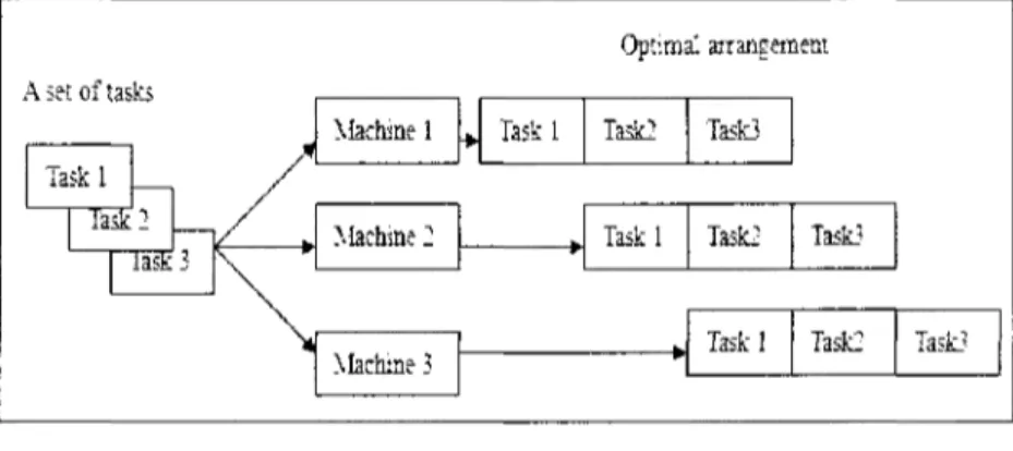
Along with the Industrial development, in the most complex environments, a single machine scheduling cannot meet the requirements of the production as in manufacturing industry, food processing industry, etc. In these industries, all task processes are the same, so we expand the production scale by adjusting the number of production lines. To schedule n independent tasks on m identical machines that operate in parallel is called the parallel machine scheduling problem, as pictured by Figure 2-2. In the case of a workshop assembly process, for instance, each task j is only allowed to be processed on a specified subset of machines. According to the processing speeds, parallel machines can be classified into identical parallel machines (the speeds of machines are the same), uniform machines (the speeds of the machines are proportionate), and unrelated machines (the speeds are not related and the processing times depend only on the jobs), respectively.

Taskl 1 iask

T

'—1

s

Figure 2-2: Parallel Machine Model

In the context of transportation, computation and logistics management, every task is independent and operations (routes, courses, etc) of every task are different. These problem common features are that every task must be processed on several different machines. The mode is called multi-jobs and non-preemptive scheduling problem model, which includes three models: flow-shop, open-shop and job-shop. In flow-shop, all jobs will be processed on all the machines in the same order such as Figure: 2-3. In this figure, we have a set of three jobs and a set of three machines. And we can notice that each job has followed a same order on the three machines.

A set of tasks Task 1 1 Task2 / / \ Machine 1 Machine ^ Machine 3 » Taskl Optimal arrangen Task: Task3 Taskl Task: Taskl lent Task? Task: Task?

Figure 2-3: Flow Shop Model

There exists within this model a special case which occurs in its own right in many applications. In this flow-shop model, jobs do not overtake other. This means that, if a job precedes another job on one machine, then this remains the same for the rest of the machines. This models scheduling processes with queuing restrictions. This model is known as the permutation flow-shop.

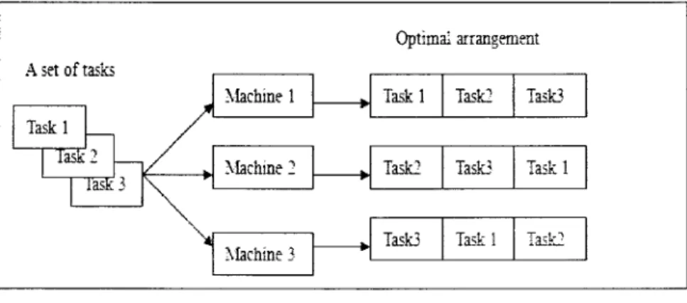
In the open-shop model, a set of jobs are processed on several machines. Each job has to be processed on each machine and does not have a fixed route. In fact, this route should be built when constructing a solution. In Figure 2-4, we have a set of three jobs and a set of three machines. We can notice that each job has followed a different sequence on the three machines.

A set of tasks Taskl lad-' iâsfc 3 Machine 1 Machine 2 Machine 3 Optimal arrangement Taskl Taski Taski Taski Task3 Taskl Task3 Taskl Task2

Figure 2-4: Open Shop Model

In job-shop model, a set of n jobs are processed on m machines. Each job consists of a fixed processing order though the machines. In Figure 2-5, we have four jobs and six machines. Each job follows a fixed route on the six machines, which is highlighted by a color. For example, a job may pass through machine 1, then machine 4, and finally machine 5.

Figure 2-5: Job Shop Model

Let us conclude this section by mentioning the fact some of the above models can be mixed together to form new models, for example one can assume that the set of job can be divided into a flow shop type and an open shop type. We can also that in a job shop model each stage can be formed by a set of parallel machines.

2.3 Basic Definitions

We present in this section some basic definitions, used in scheduling theory that we will need for the rest of this dissertation.

Definition 2-3-1: A schedule may be viewed as a way of assigning, over time, tasks to

resources. It is possible to determine planning and design for a problem by means of

calculation in advance.

A resource is a basic device where jobs are scheduled/processed/assigned [Blazewicz et ai, 2004], which is known as CPUs, memory, storage space; workshop factory. Each resource has a limited capacity, a speed and a load. The limited capacity is a number of CPUs, amount of memory, the size of storage space and so on.

The speed is defined as how quickly a job can be processed on a resource. The load measures how much of the capacity of a resource is used over a time interval. If a resource can be used by different tasks, it is called renewable; otherwise it is called nonrenewable.

Definition 2-3-2 [Fibich etal, 2005]

A machine is a set of cumulative resources (CPUs, memory, storage space, workshop

factory) with limited capacities. The characteristics of a machine include its capacity, load, speed and location, which are described by descriptors of the machine.

Defintion 2-3-3 [Fibich et al, 2005]

A job (task, activity) is a basic entity which is scheduled on the resources. A job has

specific requirements on the amount and type of resources (including machines) or

required time intervals on these resources.

A detailed description of these conditions is quite difficult to undertake. Graham et al. [1979] introduced a three-field notation to describe scheduling problems.

2.4 Three-Field Notation

Scheduling problems are often classified according to Graham's standard three-field a | /? | y notation [Graham et al., 1979], where a describes the machine environment,/? provides details of characteristics or restrictive requirements, and

y stands for the criterion performance measure.

1. The a field: The basic machine environments include single machine problems,

various types of parallel machine problems, flow shops, job shops, open shops, mixed shops and multiprocessor task systems problems.

A single machine is denoted by " 1 " in the «field to indicate that the scheduling problem is solved by one machine. If jobs are scheduled on m identical machines operating in parallel, then this denoted by Pm; with uniform machines where the speed

are proportionate ( Qm ), unrelated machines where there no special relationship

between the speeds of the machines (Rm), and flow shop, job shop, open shop with m

machines are denoted by Fm, Jm, Om, respectively.

2. The o field: It provides details of characteristics or restrictive requirements.

Details of characteristics and restrictive requirements are further described and qualified for the current resources and the environment.

- Processing Time: the time by which taken to complete a prescribed procedure. -Time delay (time lag): the time that must elapse between the completion of an operation and the beginning of the next operation of the same job.

- Breakdown (brkdwn): The breakdown indicates that the machines (resources) can break down thus not available for processing.

3. The y field: It denotes performance measures for evaluating the quality of

solutions. The performance measures define the quality of the obtained schedule based on input parameters of particular tasks and, usually, on their completion times. They take into account all the tasks existing in the system in order to estimate its

the set of jobs are as follows:

- Arrival time: Time at which a given job becomes available for processing. - Due date: Time by which a given job should be completed.

- Weight: A positive value associated with a given job to denote its relative importance or priority.

Those performances are usually given as a function of the completion times of the jobs.

Definition 2-4-1

The completion time C of a job j denotes the time at which the last operation of this

job is completed.

A list of objective criteria, commonly used in scheduling theory, could include the

following:

- Makespan: The completion time of the latest job also is known as the time difference between the start and finish of a sequence of jobs that is denoted asCmax = max C, . So the goal is to minimize C max .

- Total weighted mean completion time: The goal is to find a feasible schedule of the n jobs that minimizes

- Maximum lateness: The goal is to find a schedule which minimizes

Ln m = m a x ( Cj-dj).

- Tardiness: A job is tardy if c > d . Tardiness is defined as T j = max} 0, L j} .

If for some schedule the maximum lateness is not positive then the maximum tardiness is 0 which is obviously optimal. Otherwise the maximum lateness is positive, and so the maximum tardiness is equal to the maximum lateness.

Number of tardy jobs: we denote the number of tardy jobs by U ; .Let

U j =\ ifC; > d., otherwise. Then, the goal is to seek a schedule of the jobs so as

to minimize

2.5 Gantt Chart

Gantt chart, a useful tool for analyzing and planning more complex projects, was designed by Gantt [1916]. Gantt diagram is a type of bar chart that illustrates a graphical representation of the start and completion time of the jobs of a project, which includes two perpendicular axes. While the vertical axis represents the number of machines, its horizontal counterpart represents a time scale.

Example 2-1

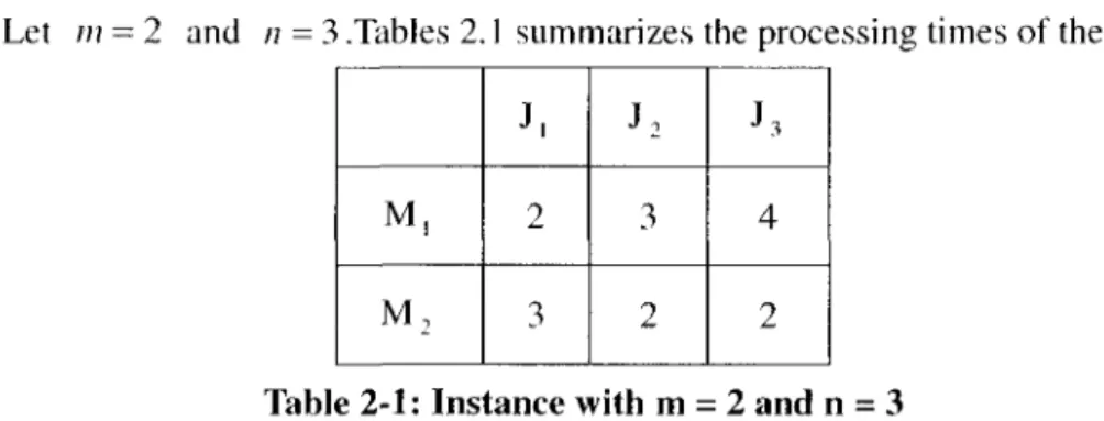
Let m = 2 and /; = 3 .Tables 2.1 summarizes the processing times of the jobs.

M, M2 J, 2 3 J2 3 2 J3 4 2

Table 2-1: Instance with m = 2 and n = 3

Figure 2-6 shows the Gantt chart associated with a scheduling solution. The Gantt chart provides a fast, intuitive way to monitor the scheduling progress and to determine where troubles are in a given solution. For this diagram, we can observe the status of each task (for e.g. start time, completion time, etc), and make time adjustments to change the processing sequence in order to obtain an optimal sequence.

M a c h i n e • M. M: l

mm

ill

m

The Gantt diagram visualizes the different orderings of jobs on machines and other information of a given solution. In what follows, the Gantt chart is used to picture the effects of time delays and idle time on the quality of a schedule.

2.6 Scheduling with time delays

In scheduling theory, some objective factors cannot be evaded in practice, such as the time spent when transmitting a work-piece after its completion on one machine to another to process; the time spent in clearing off the runway between an aircraft's landing and take-off which are controlled by the airport schedule, etc. In some cases, they have to be considered if we want to build a valid solution.

Time delays can be classified into minimal, maximal and exact time delays. In some cases, a time delay of a minimum length must elapse before handling the considered product, like when transporting products form one center to another. This is termed as the minimum time delay situation. However, if the interval between two operations is too long, it is very likely to lead to the scrap or quality decline of the processed products. Take food processing industry, where too long time of storing food makes food decay. Faced with these circumstances, an upper bound and lower bound are set on time delays, which are termed as minimum time delays and maximum time delays. In some other cases, the waiting time between the completion of an operation and the beginning of the next operation of the same job must be fixed. This is termed as the exact time delay situation. Let us note that, in general, if there are not special indications, time delays refer to the minimum time delays case. Let us consider the following instance with m = 2 machines and n = 4 jobs.

Example 2-2 M, 2 2 J2 2 2 3 2 J4 3 8 Table 2-2: An Instance with m = 2 and n = 4

An optimal solution for this problem is as illustrated by Figure 2-7.

Machine-M ,

WÊÊÈ

Trnie

Idle

Figure 2-7: Optimal schedule without time delays

Let us now consider the same instance, but with time delays considerations given as in Example 2-3. Example 2-3 Job Time delay 1 . J, 2 J: 2 J3 1 J4 3

Table 2-3: Time Delays for Example 2-2

The optimal solution becomes as in Figure 2-8.

Machine-

M,-The tsme

de'.av9 11 13 -P S Waiting when the same be ^ ^ processed on another machine

Figure 2-8: Optimal Schedule with Time Delays

2.7 A Brief introduction to the complexity theory

Computational complexity theory, an active field in theoretical computer science and mathematics, deals with the resources required during computation to

solve a given problem. To put it simply, the aim of the complexity theory is to understand the intrinsic difficulty of solving a given problem.

Definition 2-7-1

The complexity of an algorithm is the "cost" used by the algorithm to solve a given

problem. The cost can be measured by terms of executed instructions (the amount of

work the algorithm does), running time, memory consumption or something similar.

Among all "costs", we focus our attention on the running time of an algorithm. The best-case, worst-case, and average-case complexities refer to three different ways of measuring the time complexity as a function of the input size. We are more interested in understanding the upper and lower bounds on the minimum amount of time that are required by the most efficient algorithm solving a given problem. Therefore, the time complexity of an algorithm usually refers to its worst-case time complexity, unless specified otherwise. The worst-case or average-case running time or memory usage of an algorithm is often expressed as a function of the length of its input using the big O notation. In typical usage, the formal definition is not used directly; rather the O notation for a function T(n) is derived by the following simplification rules: If T(n) includes several factors, only the one with the largest growth rate is kept, and all other factors and any constants are omitted. For instance, if the execution time of an algorithm T{n) = 611* + 32 — 2« + 5 , then the worst-case

complexity is T(n) = O{n3).

Definition 2-7-2

An algorithm is said to be polynomial time if its running time is upper bounded by a

Definition 2-7-3

If a problem can be solved in polynomial time, it is called tractable; otherwise it is

called intractable.

Definition 2-7-4

A decision problem is a type of computational problem whose answer is yes or no.

Decision problems are the core objectives of study in computational complexity theory. In this section, our discussion is hence restricted to decision problems.

• P and NP classes

Definition 2-7-5

The P-class consists of all problems that can be solved in polynomial time as a

function of the size of their input.

Definition 2-7-6

If a decision problem can be solved in polynomial time, then it belongs to the P-class.

Definition 2-7-7

NP represents the class of decision problems which can be solved in polynomial

time by a non-deterministic model of computation.

From the above definitions, we can easily derive the relationship: P is included in NP, but if we do not know whether P = NP.

In 1971, Stephen Cook published a paper "The complexity of theorem proving procedures", in which he further proposed the concept of NP-completeness.

• NP-hard and NP-complete classes

Definition 2-7-8

A decision problem L is NP-complete if it is in NP and if every other problem in NP is

reducible to it.

The term "reducible" means that there exists a polynomial-time algorithm to transform an instance/G Linto an instance c e Csuch that the answer to c is YES if, and only if, the answer to / is YES.

Definition 2-7-9

NP-hardness (non-deterministic polynomial-time hardness), in computational

complexity theory, refers to a class of problems that are, informally, "at least as hard as the hardest problems in NP". A problem H is NP-hard if and only if there is an

NP-complete problem L that is polynomially reducible in time to H.

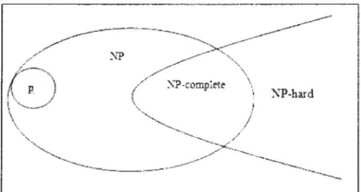
NP-complete problems are the most challenging in the NP class. A problem is NP-hard if it is at least as hard as any problem in class NP. If there is a polynomial algorithm for any NP-hard problem, then there are polynomial algorithms for all problems in NP, and hence P = NP. Figure 2-9 shows the relationship between P, NP, NP complete and NP-hard classes.

/ I \ p X \ \ NP \ XP-complete NP-hard

2.8 Analysis of Scheduling Problems

In this section, we describe the way to analyze or deal with deterministic scheduling problems. In this dissertation, we have limited our study to "deterministic" scheduling problems. In other words, all parameters are assumed to be known and fixed in advance.

Generally speaking, the idea of analyzing deterministic scheduling problems is to find the appropriate solution according to their respective characteristics. In most cases, the time "cost" is limited, so that only low order polynomial time algorithms may be used. Thereby, understanding the complexity of algorithm is very important and is also the basis for further analysis. In section 2.6, we have introduced some categories of the class complexity (P class, NP-complete class, and NP-hard class). The complexity of problems is the basis for further analyzing the problem solving process. If the problem is in the class P, then a polynomial time algorithm must already have been found. Its usefulness depends on the order of its worst-case complexity function and on the particular application. Except the worst-case complexity analysis, probabilistic analysis of algorithms is a common approach to estimate the computational complexity of an algorithm..

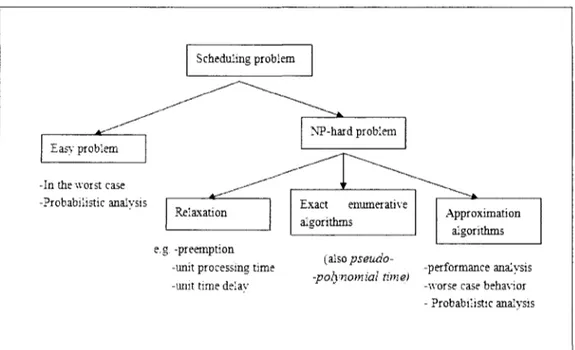
As illustrated in Figure 2-10, if a problem is NP-complete or NP-hard, then either of following approaches is used in order to solve it: exact method, relaxation, approximation method, and pseudo-polynomial method.

Figure 2-10 shows a schematic view to analyze scheduling problems. These methods are further explained in the following sections.

Scheduling problem

îasy problem

-In the worst case -Probabilistic analysis

Relaxation Exact enumerathe algorithms

e.g. -preemption -unit processing time -unit time delav

Approximation algorithms

(aiso pseutio--po'iynomial time)

-performance analysis -worse case behavior - Probabilistic analysis

Figure 2-10: Analysis of Scheduling Problems

2.8.1 Exact methods

An exact algorithm is an algorithm that can obtain an optimal solution to a given problem. This class of algorithms is divided into polynomial time algorithms and enumerative algorithms. For some special structured problems, we may find polynomial time algorithms to solve them. For example, when the time delays are ignored, an optimal solution to two-machine open shop problems can be obtained in polynomial time by a simple algorithm. However, form > 3, the open shop scheduling problem becomes NP-complete [Pinedo, 1995].

Let us observe that most scheduling problems are NP-hard problems, which means that the only algorithms we have at hand to solve these problems need exponential running time. Such algorithms are mainly enumerative algorithms, linear programming, and dynamic programming.

2.8.2 Relaxation

We may try to relax some constraints imposed on the original problem in order to reduce the difficulty of its resolution. The solution may be equal to or more closer

to the optimal solution of problem. Within the scheduling context, these relaxations may include:

- allowing preemptions,

- assuming unit-time operations, - assuming simpler precedence graphs, - etc.

2.8.3 Pseudo-Polynomial Algorithms

Although all NP-hard problems are computationally hard, some of them may be solved efficiently in practice. This is because the time complexity of those algorithms mainly depends on the input length and the maximal number. In practice, the maximal number is not large, and is usually bounded by a constant; this leaves us with a polynomial algorithm. This is where the name of pseudo-polynomial algorithm comes from. It does not mean the algorithm really is a polynomial algorithm.

2.8.4 Approximation Algorithms

It is time consuming (and thus difficult) to find optimal solutions to NP-hard problems. Therefore, the approximation approach becomes almost an inevitable choice. The approximation algorithm generally falls into heuristic algorithm and meta-heuristic algorithm. These approaches are described in details in Section 2.9.

Generally speaking, heuristic algorithms are used to solve special problems, but the improvement space of a heuristic algorithm is limited, so researches often try to find a new and better algorithm to solve it. The same problem is often able to be solved by several different heuristic algorithms; moreover we have difficulties in intuitively judging which one is better. For some cases, the results of some heuristic algorithms are better, but for other cases, some contrary conclusions may be drawn. Thereby, some uniform measurement standards and calculating methods are indispensable. We commonly evaluate the performances of different heuristic algorithms by using two methods: the Analytic Approach and the Empirical Approach.

2.8.4.1 Analytic Approach

The analytic approach is about finding the distance between an optimal solution and the solution produced by a heuristic algorithm. The commonly used methods include the worst-case analysis and probabilistic analysis.

• Worst-case Analysis

The quality of a given heuristic is measured by the maximal distance between the optimal solution and the solution produced by the heuristic under study.

Usually, the maximal distance is measured by the relative error between the two solutions. If SH and S denote the makespan produced by heuristic H and an

optimal solution, respectively, then the goal is to find a ratio performance guarantee (or worst case bound) p such that the following relationship holds:

where Cmax (5) denotes the makespan of schedule S.

• Probabilistic Analysis

Probabilistic analysis starts from an assumption about a probabilistic distribution of the set of all possible inputs. This model usually assumes that all parameter values are realizations of independent probabilistic variables of the same distribution function. This assumption is then used to design an efficient algorithm or to derive the complexity of a known algorithm. Then for an instance / of the considered optimization problem (n being a number of generated parameters) a probabilistic analysis is performed. The result is an asymptotic value OPT ( / ) expressed in terms of problem parameters. Then, algorithm A is probabilistically evaluated by comparing solution values (A ( / ) being an independent probabilistic variables) with OPT ( / ) [Rin87]. The two evaluation criteria used are absolute error and relative error. The absolute error is defined as the difference between the approximate and optimal

solution values

an=A(I")-OPT(In).

The relative error is defined as the ratio of the absolute error and the optimal solution value

AUJ-OPTUJ

b =•

OPT{1N)

2.8.4.2 Experimental Approach

The experimental approach is based running the corresponding algorithm on a large number of effective data to evaluate its performance. This approach is mainly used to compare multiple heuristic algorithms.

Let us note that the analytic and the experimental approaches are complementary: the former proves strong theoretical foundations under some hypotheses, and the latter shows the practical performance tendency of the considered algorithm.

In Section 4.3.2., we present a complete example to compare two heuristic algorithms.

2.9 Description of an Exact and a Heuristic Approach

In the above section, we have mentioned different approaches to solve a scheduling problem. In this section, we will give more details on some of these methods.

2.9.1 Exact Algorithms

In addition to special cases, enumeration (brute force search) algorithm is a very general problem-solving technique for obtaining exact solutions that consists of systematically enumerating all possible candidates for the solution and checking whether each candidate satisfies the problem's statement. Enumeration algorithm mainly includes branch and bound, dynamic programming and so on. In what follows, we present in more details the algorithm of branch and bound (B&B for short), which is used extensively in practice.

• Branch and Bound

Branch and Bound (B&B) is the most commonly used enumeration algorithms for combinatorial optimization problem (NP-hard problems) to generate an optimal solution.

The efficiency of a branch and bound method is determined by the branching efficiency and pruning ability. The branching efficiency is determined by the branching strategy and searching strategy. The pruning ability is determined by the values of the upper bound, lower bound and the effect of dominance rule at hand. An upper bound corresponds to the value produced by an arbitrary schedule. A lower bound value corresponds to the smallest value that can be achieved by any solution, whereas a dominance rule states that any solution cannot be better than the one produced by the solution with a certain property.

The method of branch and bound was used for the first time by Danzig, Fulkerson, and Johnson [1995] to solve the problem of traveling salesman (TSP).

The idea of the method of branch and bound is to first confirm the upper and lower bounds of the goal values and then cut off some branches of the search tree while searching, to improve the efficiency of the search.

1. Bounding

A lower bound represents the smallest value that can be obtained by a feasible solution. As far as the method of branch and bound is concerned, if the lower bound of a given node, in a search tree, is not smaller than the known upper bound, a downward search from this node will not be needed. Therefore, if a superior upper bound can be produced, then many unnecessary listing calculations will be eliminated.

2. Search Strategy

The searching ways are divided into two categories, depth-first search and breadth-first search.

Depth-First-Search (DFS) starts at the root (selecting some node as the root in the graph case) and explores as far as possible along each branch before backtracking.

The nodes are visited in the order A , B , C , D

Depth-First-Search (DFS)

Breadth-First-Search (BFS) begins at the root node and explores all the neighboring nodes. Then for each of those nearest nodes, it explores their unexplored neighbor nodes, and so on, until it finds the goal.

The nodes are visited in the order A. B.D. C

Breadth-First-Search (DFS) Branching

The operating principle of pruning is like a running maze. If we regard the searching process as a tree traversal, pruning literally means "cutting off the "branches" that our needed solutions cannot reach, the dead ends in a maze, to reduce the searching time.

Of course, not all the branches can be cut off. However, more branches are pruned, the faster is the method. Pruning principle is as follows:

3.1. Correctness

As observed above, not all branches can be cut off. If the optimal solution is cut off, then the pruning does not make any sense. Thus, the precondition for pruning is ensuring that correct results will not be lost.

3.2. Efficiency

Therefore, it is equally important how to strike the balance between optimization and efficiency to lower the time complexity of program as much as possible. If a judgment for pruning produces a very good result, but it has taken much time to make the judgment and the comparison, with the result that there is no difference between the operations of the optimized program and the original one; it is more loss than gain.

2.9.2 Heuristic Algorithms

The heuristic approach (from the greek "heuriskein" meaning "to discover") is based on experience techniques that help in problem solving, learning and discovery. Heuristics are "rules of thumb", educated guesses, intuitive judgments or simply common sense rather than by following some pre-established formula.

The core idea of a constructive heuristic is to build step by step a solution to problem. In other words, each step of the algorithm is only to consider the next step according to a given rule. The priority rule provides specific strategies for the sequence in which jobs should be processed according to some rules such as Shortest Processing Time (SPT), Earliest Due Date (EDD), and so on.

Although an optimal solution to every combinatorial problem can be found, some of these would be impractically slow for NP-hard (NPC) problems, since it is unlikely that there can be efficient exact algorithms to solve these problems. However, for some special cases, heuristic (suboptimal) algorithms can find the optimal (or close to optimal) solution in reasonable time complexity. A worst case analysis is commonly used to study the performance of these algorithms.

• Local Search Methods

Local search can solve some problems that find a maximum solution among a number of candidate solutions (candidate solution is a member of a set of possible neighborhood solutions to a given problem). Neighborhood search is continuously searching in the neighborhood domain of the current solution.

Local search algorithm only searches the neighborhood domain of the best present solution (like the above example), and if the new domain does not have a value that is better than the present value, then the iterative process will be stopped. Local search algorithms are typically local optimal solution algorithm, which is simple and rapid, but the accuracy of results may be poor. A computational simulation is commonly used to study the performance of these algorithms.

2.9.3 Meta-heuristic Algorithms

Generally, the heuristic algorithms have good results that are used to solve specific objectives but not all. For example, the results of some heuristic algorithms may depend on the selection of an initial point; if the objective function and constraints have multiple or sharp peaks, the quality of the result may become unstable. The computational drawbacks of existing heuristic methods have forced researchers to improve it.

In a general framework optimization heuristics are also called meta-heuristics which can be considered as a general skeleton of an algorithm applicable to a wide range of problems.

The meta-heuristics algorithms are that they combine rules and randomness to imitate natural phenomena such as the genetic algorithm (GA) proposed by [Holland, 1975] (the evolutionary), tabu search proposed by [Glover, 1986] (animal behavior) and simulated annealing proposed by [Kirkpatrick et al, 1983] (the physical annealing process), etc. These meta-heuristics algorithms are theoretically convergent, that is if the computation time tends to infinity, it will be able to find the global optimum under certain conditions. However, these conditions are rarely verified in practice.

The meta-heuristics includes a new random initial solution (or the solution of a constructive heuristic) and a black-box procedure (iterative search). The common method used to analyze the performance of these algorithms is the computational simulation.

2.9.3.1 Simulated Annealing

The idea of simulated annealing (SA) is presented by [Metropolis, 1953] at first and applied on combinational optimization problem by [Kirkpatrick, 1983]. The basic starting point of SA is based on metal (solid) in annealing process that is a process for finding low energy states of physical substance that refers to a process when physical substances are raised to a high temperature and then gradually cooled until thermal equilibrium is reached. The process can be simulated by Monte Carlo method, which initially serves the function that it is applied to find the equilibrium configuration of a set of atoms at a given temperature (R = exp(£; — E)lkT, where £\ denotes the

energy in / state; T denotes temperature; k is the cooling factor).

In 1983, Kirkpatrick first introduced the Metropolis rule to combinational optimization problems. This algorithm process is called Simulated Annealing algorithm. In combinatorial optimization problems, an initial value / and its objective function/f/j correspond separately to a state / and its energy Ej and use two control parameter

ta,tj to simulate initial temperature and terminated temperature. Repeat the process:

"create—judge—accept/abandon" until some stopping criterion is achieved. The basic annealing process for open shop problems may be as follows.

I--rai)do:r; sequence 1" " ~ tuK

Imtï-iî îemperaîure J"*™ 7*. Temiiiaatect EeinperaEme T . * ~ X Cooling factor ci " — a

,-Repeat

Gene:ate i randc-srs neighbor t\j> f'Oinf-.iY'

If_}/:"- " O then accept tlie nev,- sequence {£"— Sj),f(!)--f!'j>J

Else

\t\\f->0

then-gi*t a random number h e (O.I '»,-If H ~exp f-.-SfT)

Then accept the a e w sequence (f".— fi'j) ;gj)"^j». If T~- T then T ~Ct

Tr-until (termination-condition);

2.9.3.2 Genetic Algorithms

Genetic Algorithms (GA) are adaptive heuristic search algorithm premised on the evolutionary ideas of natural selection and genetic that was invented by John Holland in the 1960s, and was developed with his students and colleagues at the University of Michigan, in the 1970s. Genetic algorithms are categorized as global search heuristics. The basic concept of GA is designed to simulate processes in natural system necessary for evolution, specifically those that follow the principles first laid down by Charles Darwin of survival of the fittest. As such, they represent an intelligent exploitation of a random search within a defined search space to solve a problem.

Genetic algorithms are implemented in a computer simulation in which a population of abstract representations (called chromosomes or the genotype of the genome) of candidate solutions (called individuals, creatures, or phenotypes) to an optimization problem evolves toward better solutions. Traditionally, solutions are represented in binary as strings of Os and Is, but other encodings are also possible. The evolution usually starts from a population of randomly generated individuals and happens in generations. In each generation, the fitness of every individual in the population is evaluated, multiple individuals are stochastically selected from the current population (based on their fitness), and modified (recombined and possibly randomly mutated) to form a new population. The new population is then used in the next iteration of the algorithm. Commonly, the algorithm terminates when either a maximum number of generations has been produced, or a satisfactory fitness level has been reached for the population. If the algorithm has terminated due to a maximum number of generations, a satisfactory solution may or may not have been reached.

A basic genetic algorithm comprises three genetic operators: Selection, Crossover, and Mutation.

a. Selection

This operator selects the chromosome in the population for reproduction. Based on the survival-of-the-fittest strategy, the more fit the chromosome, the bigger

chance to be selected for reproduction. The most commonly used strategy to select pairs of individuals is the method of roulette-wheel selection, in which every string is assigned a slot in a simulated wheel sized in proportion to the string's relative fitness. This ensures that highly fit strings have a greater probability to be selected to form the next generation through crossover and mutation.

b. Crossover

Crossover is a genetic operator that combines two chromosomes to produce one or two new chromosomes. The idea behind crossover is that the new chromosome may be better than both of the parents if it takes the best characteristics from each of the parents. Crossover occurs during evolution according to a user-definable crossover probability includes the following types of crossover.

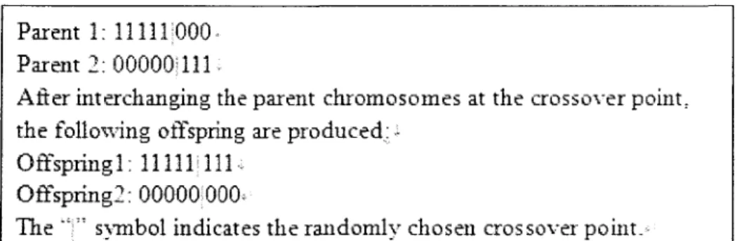
b.l. Single Point Crossover

After randomly choosing a crossover point on two parent chromosomes and inter changing them at the crossover point, two offspring are produced. End each of them inherits the genes of its parent before the crossover point and the ones of the other parent after the crossover point. Consider the following two parents selected for a crossover.

Parent 1: 11111:000. Parent 2:000001111:

After interchanging the parent chromosomes at the crossover point, the following offspring are produced:}

Offspring 1: 11 111! I l l -Offspring2:

OOOOOjOOO*-The "i" symbol indicates the randomly chosen crossover point.*

Figure 2-8: Single Point Crossover b.2. Two Point Crossover

After randomly choosing two crossover points on two parent chromosomes and interchanging them at the crossover points, two offspring are produced. Each of them

inherits from its parent the genes except between the two points, and from the other parent the genes between the two points. Consider the following two parents selected for two crossovers.

Parent 1: 111} 11 Parent 2: 000 00 After interchang crossover points Offspring 1: 111 Offspring 2: 000 The " " symbol i 000 4. UU

ing the parent chromosomes between the . the following offspring are produced:

-OOiOOO* 111 111*1

ndicates the randomly chosen crossover point-*

Figure 2-9: Two Point Crossover b.3. Uniform Crossover

Bits are randomly copied from the first or the second parent. Consider the following two parents selected for a crossover.

Parent 1: Parent 2:

12345676-34214575.

If the mixing ratio is 0.5. offspring

parent 2. Offspring Offspring

approximately will come from parent 1 and the Below is a possible 1: 1435576^ 2: 3224675--set of offspring half-other after

of the genes in the half will come from uniform crossover:

Figure 2-10: Uniform Crossover c. Mutation

On certain odds, there is the possibility for every gene in the sequence to change. This is a method that can avoid the minimum in local. In scheduling, this change may be randomly exchanging the processing orders of two tasks. A simple genetic algorithm for the open shop problem is as described by Algorithm 2-2.

Generate random population of n chromosomes (suitable solutions for the problem) ••

Evaluate the fitness f(x) of each chromosome x in the population^ Repeat >!

Select two parent chromosomes from a population according to their fitness (the better fitness, the bigger chance to be selected). • Setup a crossover probability: two parent chromosomes form two new

offspring (children) by a certain crossover point. If no crossover is performed, an offspring is the exact copy of

parents.-With a mutation probability, mutate two new offspring at each locus (position in

chromosome).-Place new offspring in the new population to replace the old generation If the end condition is satisfied; stop else go repeat:*'

Algorithm 2-2: The Basic Genetic Algorithm Process

2.9.3.3 Tabu search method

The basic principle of tabu search (TS) method is based on classical local search method (LS) improvement techniques and to overcome local optimal by crossing boundaries of feasibility. The essential feature of a TS method includes allowing non-improving moves, the systematic use of memory and relevant restrictions for improving the efficiency of the exploration process. Tabu search was presented by [Glover, 1986, 1989, 1990]. Let us note that the basic ideas of the method have also been advanced by [Hansen, 1986].

In order to avoid local convergence, the idea that "inferior solution" can be accepted to some extent is derived. The important objective of the method reasonably increases the scope of neighborhood domain and avoids searching as far as possible in the found neighborhood. The components of TS include tabu list (memory length), tabu length and candidates swap and aspiration criteria. Tabu list is a short-term memory which contains the solutions that have been visited in the recent past (candidate swaps). In the tabu list, certain moves are prohibited to be visited unless the move is "best so far". The time of the move is decided by the tabu length. The basic tabu search procedure for open shop might be as follows.

Obtain a random initial sequences Clear up the Tabu list:

Repeat •

ïïï)

Select anew minimum sequence f(j) in the neighborhood of Si); If jSj)<best j q j a r then

begin

iSX f(j) take piace of the oldest

end else begin

if Sj) « not m the Tabu flj) take place of the end:

untii (termination-condition):

sequence in the Tabu list:

list then

oldest sequence in the Tabu iist;

Algorithm 2-3: The Basic Tabu Search Process

In recent years, two ideas have been incorporated into the TS method:

intensification and diversification, in the perspective of improving the quality of the results produced by that method.

The idea of intensification is to explore in depth the best solution that have been searched out and its neighborhood. The idea of diversification is to force to search into previously unexplored areas of the search space in order to avoid the local convergence.

Intensification procedure

1 Record the current sequence

2 Insert job k in other (n-l) jobs to obtain a set of new sequence;

3 Find the shortest sequence in this set;

4 Repeat step lto 3 until the number of the shortest sequences is—.

Diversification procedure 1 Save the best sequence;

2 Generate at random an initial sequence;

N

3 Regenerate — random permutations;

Chapter 3

The Two-Machine

Open Shop without

3.1 Introduction

Let us recall the description of an open shop scheduling problem. A set of «jobs j ={y],7,,...,7i i} has to be processed on a set of m machinesM = {M],M2,...,M „,}•

The routing of the jobs through the machines is not known in advance. In fact, it is part of the solution as it becomes known during the process of building the schedule.

Let us mention that open shop scheduling problems may arise in many applications. Take a large aircraft garage with specialized work-centers for example. An airplane may require repairs on its engine and electrical circuit system. These two tasks may be fulfilled in any order. Other examples of open shop problems include examination scheduling, testing repair operation scheduling, satellite communications, semiconductor manufacturing, quality control centers, etc.

The two-machine open shop problem without time delays (O2 || Cmax ) describes

the simplest and easiest state of the problem. So, in some cases, the result of O2 || Cmax problem is considered as a lower for other complex two-machine open

shop problems, and may also provide an important theoretical basis for solving other complex open shop problems.

In this section, the Gonzalez-Sahni algorithm and the Schrage-Pinedo Algorithm (LAPT) are presented to solve the 0 , || Cnra algorithm. We restate the latter algorithm

for an easy implementation and give a proof of its optimality.

3.2 Gonzalez-Sahni Algorithm

Gonzalez & Sahni [1976] present a polynomial algorithm to generate an optimal solution for the O2 || Cmax problem, denoted hereafter as GS algorithm.

• The basic idea of GS algorithm

Let a • - p{j ,b/ = /?•,•; G S a l g o r i t h m consists of splitting t h e set J of jobs into

from the "middle", with jobs from <p added on at the right and those from y at the left. Finally, some finishing touches involving only the first and last jobs in the schedule are made. The algorithm can be described as follows:

Begin

Choose any two jobs J > and J. for which a ;. 2. max {b.} and b_ > max {a ,} ;

Set/ : = 7 - { J , , J;} :

Construct separate schedules for <p -* {J . } and y _ {J . }; Join both schedules:

Move tasks from y „ {J } processed on machine 2 to the right;

Change the order of processing on machine 2 in such a wav that J;. is processed

first on this machine; End

Algorithm 3-1: GS algorithm Example 3.1

Let us illustrate the GS algorithm on an instance of the two-machine open shop with four jobs. The processing times are as follow.

M, M 3 J, 2 6 J2 6 2

h

Table 3-1 : Processing times for an instance with 4 jobs

W e h a v e t h a t <p = {J-,,J^} ; y = {Jt,JA} ; bt - 74( & , > m a x { «;. } ) . It t h e n f o l l o w s

.1,50

y u {Jk} = {/?,,bA} ; see Figure 3-1.

that b, =J4(b! > m a x { « }); ak = J3(ak > m a x { / ? . } ) ;

liillllliiii

r/j S/s f/j r/j r/j r/, S/J Ao '/; f/S'/s '/;

Figure 3-1: Two partial schedules

Both schedules are joined and the order of processing on machine 2 is changed in such a way that b3 is processed first on this machine, as illustrated by Figure 3-2.

Figure 3-2: Optimal Solution produced by the GS algorithm

3.3 Pinedo-Schrage algorithm

The optimal solution of the above problem can be found in another way. Indeed, Pinedo and Schrage [Pindedo, 1982] presents LAPT (Longest Alternate Processing Time) algorithm. The idea of this algorithm is as follows.

1. Let p be the job with the longest processing time. If this happens on machine Ml (M2), then process job/? on machine M2 (Ml).

2. Process the rest of the jobs arbitrarily on both machines as soon as they become free.

3. Process job/? on machine M2 (Ml) either as the last job or before the last job which is being processed on machine M l .

LAPT Algorithm

At time 0, J4is processed on Ml, with a3 =8,and M2 is idle. So7,is processed on

M2; at time 2, Ml is idle and£3 = 7. But because 73 is being processed on M2, bx — 6,

so7, is processed on Ml. This process is repeated until all jobs are completed on both machines. In the end, we get the following solution as in Fig 3-3.

M l -" M2-<-L...J

+• Illli

WE

il

f l

Figure 3-3: Optimal Solution produced by the LAPT algorithm

In what follows, we propose a simpler way to describe the above algorithm. Our proposal is twofold: the algorithm is easy to implement and prove its optimality. First, let us define the following.

Definition 3-3-1

In a two-machine open shop problem, one of the operations of a job is going to be

processed before the other operation. Such an operation is called the first operation;

the other one is called the second operation.

For an easy implementation, below is another way of stating LAPT algorithm:

1. LetpM=max { p :j ; i=l,2;j=l...n};

2. Process job k first on machine M(3-/;j; 3. For ( i=l ; i<n ;i++) with i not equal to k;

Process first operation of job / on the first available machine; 4. Process job k on machine /?;

5. For ( i=l ; i<n ;i++) with / not equal to k

Process second operation of job i on the first available machine;

Once again, let us run LAPT algorithm on Example 3-1. Let us denote phk =max{pu,pi2,pl3,pu,p2i, p22,p23, p2A} = pn.First, J^ is processed on

M2. Second, the first operations of Jf,J2,J4 are processed on the first available

machine. Third, second operation of 73 is processed on M l . At last, second

operations of J],J2,JA are processed on the first available machine. We therefore

get the following optimal solution:

• M l -

1

•

HI

jrrn !

n s

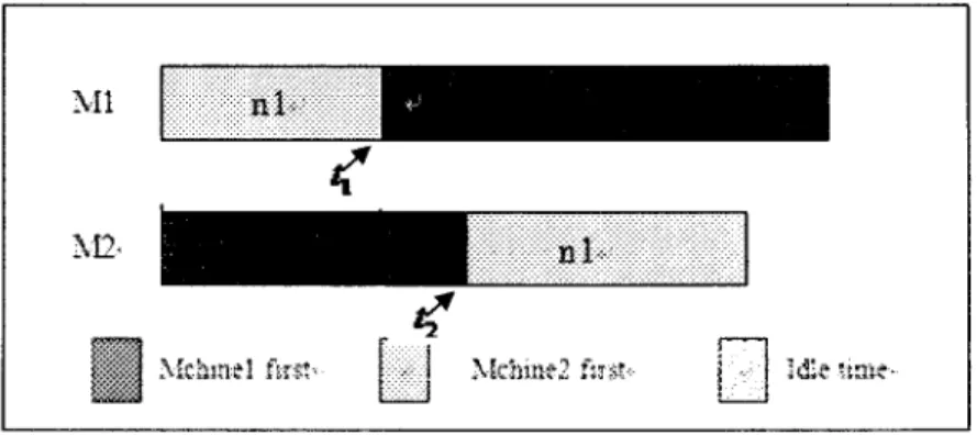
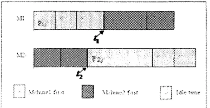
Figure 3-4: Optimal solution produced by the modified LAPT algorithm Proof of optimality: Let n, and n2 be the number of first operations processed on

Ml and M2, respectively. Let also ?, and f, be the time at which first operations on Ml and M2 are completed on Ml and M2, respectively. Let us recall that the algorithm process first operation greedily on both machines. This means that the next first operation is always processed on the first free machine. Let us distinguish the following two cases when it comes to process the second operations.

Case 1: nt = 1 and /;, > 1 :We distinguish two sub-cases either /, > t2ortx < t2.

Ml

Mi-ni: 1

•

naif-Figure 3-5: Optimal Solution for Case 1 (r, <t2)

Since f, <t2., then second operation of jobs processed on machine 1 can be processed

without an idle time. If C max ( / ) denotes the generated makespan for instance /,

then we have

which is nothing else than one of the lower bounds given above. Therefore, this solution is optimal.

Subcase 1.2. t] >t^: In this case, job 1 may cause an idle time, if the processing of

its operations is bigger than those of the first operations of jobs processed on M2. This case is shown by Figure 3-6.

li'.t itnie

Figure 3-6: Optimal Solution for Case 1 (r, > t2)

If C max ( / ) denotes the generated makespan for instance /, then have that

which is nothing else than one of the lower bounds given above. Therefore, this solution is optimal. Now, if there is no idle time on two machines, we have that

n n

Cmax (7) = m a X( Z Ptj ' Z P2j),

which is nothing else than one of the lower bound given above. Thus, the optimality of the solution follows immediately.

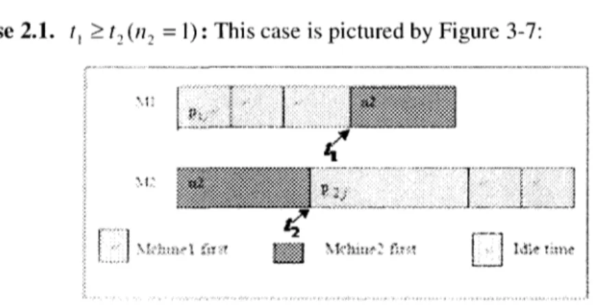
Case 2. n, > 1, n 2 > 1 : We distinguish four sub-cases:

Subcase 2.1. /, > t2 (n2 = 1) : This case is pictured by Figure 3-7:

\%ih>xtt\ inn

Figure 3-7: The Optimal Solution for Case 2 (f, > t2(n2 = 1))

Obviously, processing time p2j is bigger than the other operation processing times.

Therefore, r, + /?->,- > ?, • It then follows that second operations of jobs processed on M l or M2 can be processed without idle time. If C max ( / ) denotes the generated

makespan of instance /, then we have

n

ij ' Z

_!i_i

L

\ 1 - Î I =

Figure 3-8: Optimal Solution for Case 2 (f, > t2(n2 > 1))

Since/^T;- is bigger than the other operations, then?-, + p^ > r,, so second operations

of jobs processed on Ml and M2 can be processed without idle time. If C max ( / ) denotes the generated makespan of instance /, then we have

= max{ _p2j

7=1

Subcase 2.3. t] <t-,i If there is no idle time on M l , then this case is pictured by

Figure 3-9.

Figure 3- 9: The Optimal solution for Case 2 (f, <t2)

Since second operations of jobs processed on M2 are processed without idle time, then, if C m;ix ( / ) denotes the generated makespan of instance /, then we have that

7=1 7=1

Subcase 2.4. /, < t2 : Now, if there is an idle time on M1, then this case is pictured by

Figure 3-10: Optimal Solution for Case 2 (f, < t2)

Since we have that p , ; is bigger than the rest of the processing times, then

12 + p^ j > y pt. + possible idle time.

So, if C m.lx ( 7 ) denotes again the generated makespan of instance 7, then we have

Cm a, ( / ) = Ë P 2 J

-In any case, we have shown that the makespan generated is a lower bound. Therefore, the optimality of algorithm follows.

3.3.1 Experimental study

In order to compare the running time of the two algorithms, we run GS algorithm and the new version of LAPT algorithm on the same input data. Due to the fact that both algorithms produce optimal solutions, we only care about their running times. The conducted experiment witnessed 6 stages, where the sizes of problem successively are 50, 100, 200, 500, 800, and 1000, as shown in Table 3.2. For each size, 10 sets of data were generated at random from [1,100]. Column 2 and column 3 of Table 3.2 present, for each size, average running times of GS and LAPT algorithms, respectively. The algorithm was implemented in Visual C++ 6.0 and the tests were run on a personnel computer with a 1.66 GHz Intel® Core™ Duo CPU on the MS Windows XP operating system. The results of the experiment are summarized in Table 3-2.

Value of N 50 100 200 500 800 1000 GS algorithm 0.09765 0.09829 0.10262 0.10451 0.10675 0.10895 LAPT algorithm 0.09457 0.09712 0.09809 0.10101 0.10356 0.10543

Table 3- 2: The running times of GS and LAPT algorithms Discussion

From the structure perspective, LAPT algorithm is better than GS algorithm. In the latter algorithm, all jobs can be divided into two groups ((/>, y)and find, in each group, two jobs meeting conditions ak >max{/? }./?, >max{«.}and place them on the

corresponding positions to process. However, in the LAPT algorithm, we only need to find the maximum processing time of the whole set of the jobs

When comparing these two algorithms, from the running times point of view, then, without a surprise, LAPT algorithm outperforms slightly better GS algorithm, as we can see from the results of Table 3-2 (even though, this difference is not significant).

Chapter 4

The Two-Machine Open

Shop With Symmetric