A Multiscale Approach for Statistical Characterization of Functional Images

This is an author-deposited version published in: http://oatao.univ-toulouse.fr/ Eprints ID: 8348

To link to this article: DOI: 10.1198/jcgs.2009.0013 URL: http://dx.doi.org/10.1198/jcgs.2009.0013

To cite this version: Antoniadis, Anestis and Bigot, Jérémie and Von Sachs, Rainer A Multiscale Approach for Statistical Characterization of

Functional Images. (2009) Journal of Computational and Graphical

Statistics, vol. 18 (n° 1). pp. 216-237. ISSN 1061-8600

O

pen

A

rchive

T

oulouse

A

rchive

O

uverte (

OATAO

)

OATAO is an open access repository that collects the work of Toulouse researchers and makes it freely available over the web where possible.

Any correspondence concerning this service should be sent to the repository administrator: staff-oatao@listes-diff.inp-toulouse.fr

A Multiscale Approach for Statistical

Characterization of Functional Images

Anestis A

, Jérémie B

, and Rainer

S

This article presents a new methodology for improving the characterization of pixels in functional imaging, formulated as a spatial curve clustering problem. Our method op-erates on curves as a unit. It is nonparametric and involves multiple stages: (i) wavelet thresholding, aggregation, and Neyman truncation to effectively reduce dimensional-ity; (ii) clustering based on an extended EM algorithm; and (iii) multiscale penalized dyadic partitioning to create a spatial segmentation. We motivate the different stages with theoretical considerations and arguments, and illustrate the overall procedure on simulated and real datasets. Our method appears to offer substantial improvements over monoscale pixel-wise methods.

An Appendix which gives some theoretical justifications of the methodology, com-puter code, documentation and dataset are available in the online supplements.

Key Words: Aggregation; Mixture model; Multiresolution trees; Recursive dyadic

partition; Wavelets.

1. INTRODUCTION

We consider a problem in image segmentation in which the goal is to determine and la-bel a relatively small number of homogeneous subregions in an image based on functional, pixel-wise, intensity measurements. Traditional segmentation algorithms operate on uni-variate or on multiuni-variate pixel-wise measurements of fixed dimensionality and are not tai-lored to operate on curves as a unit, proceeding without taking into account the functional

Anestis Antoniadis is Professor, Laboratoire Jean Kuntzmann, Universite Joseph Fourier, Tour IRMA, B.P. 53, 38041 Grenoble Cedex 9, France (E-mail: Anestis.Antoniadis@imag.fr). Jérémie Bigot is Maître de con-férence, Department of Probability and Statistics, University Paul Sabatier, Institut of Mathematics of Toulouse, Toulouse, 31062, France (E-mail: Jeremie.Bigot@math.ups-tlse.fr). Rainer von Sachs is Professor, Université catholique de Louvain, Institut de statistique, Voie du Romain Pays 20, Louvain-la-Neuve, 1348, Belgium (E-mail:rvs@uclouvain.be).

structure of the data. This article seeks to address such problems. An example that high-lights the interest of such a methodology is brain tumor diagnostic imaging where the aim is to detect the presence of tumors and to provide insights about their types using magnetic resonance spectroscopy imaging (MRSI). This records spectra from voxels in a specific selected region of the brain that contains metabolic information about the volume in which they are measured. It can be especially helpful in the identification of heterogeneity in the tumorous part of the brain, because changes in the tissue structure can be assessed on a metabolic level. Another example is satellite remote sensing images of landscapes.

As noted from these examples, the high dimensionality and (typically) large noise that characterize such functional data make it difficult to classify the functional image con-tent, particularly when it needs to be clustered into a finite but unknown number of classes (unsupervised learning). In many applications the measured curves tend to be spiky and this requires flexible adaptive modeling of their variations. We will adopt a nonparamet-ric point of view to reduce the functional dimensionality of the observed pixel intensity curves, modeled as signal plus noise. There are many pixel curves, and during cluster-ing we need to combine information from all of them into a common representation, so we need a dimensionality reduction procedure that allows combination with modern de-noising techniques. This leads us to an “aggregation” technique (Bunea, Tsybakov, and Wegkamp2007) of nonlinear wavelet threshold estimators for each of the intensity curves. The reduced dimensionality after aggregation is still too large, so we apply Neyman trun-cation tests (Fan1996) on the significance of the resulting thresholded coefficients. Here “significance” is to be understood with respect to ability to discriminate between different class memberships. To cope with test multiplicity we use false discovery rate (FDR) ideas to control the level of the test. Using wavelet threshold estimators allows three attractive features to be combined: wavelets provide orthogonal bases that are ideal for dimensional-ity reduction by means of sparse representations; they allow for powerful denoising; they allow both heteroscedasticity and serial correlation to be included in the model without losing independence of empirical wavelet coefficients over locations within a fixed scale.

Our clustering mechanism uses an EM algorithm to estimate a Gaussian mixture model in the domain of the discrete wavelet transform of the pixel intensity curves. This clustering step uses the fact that all curves have a common “reduced” dimensionality to encode the location of the wavelet coefficients determined in the preceding dimensionality reduction step. To allow selecting the number of cluster classes from the data we use the refined EM algorithm of Law, Figueiredo, and Jain (2004).

Concerning segmentation, our point of reference for comparison is the monoscale statis-tical model that is typically used to remove noise and to help extract structure in the under-lying measurements. These methods work at pixel-level resolution and result in a low de-gree of aggregation of the information underlying the data because the appropriate choice of scale usually varies with spatial location. Monoscale approaches are the basis of a va-riety of existing methods, including ones based on maximum likelihood, decision trees, nearest neighbors, and neural networks. Consider, for instance, the example displayed in Figure 1 (this is in fact the first example in Section 3 on numerical results; a detailed description can be found there). In Figure 1(left), the image consists of individual pixels

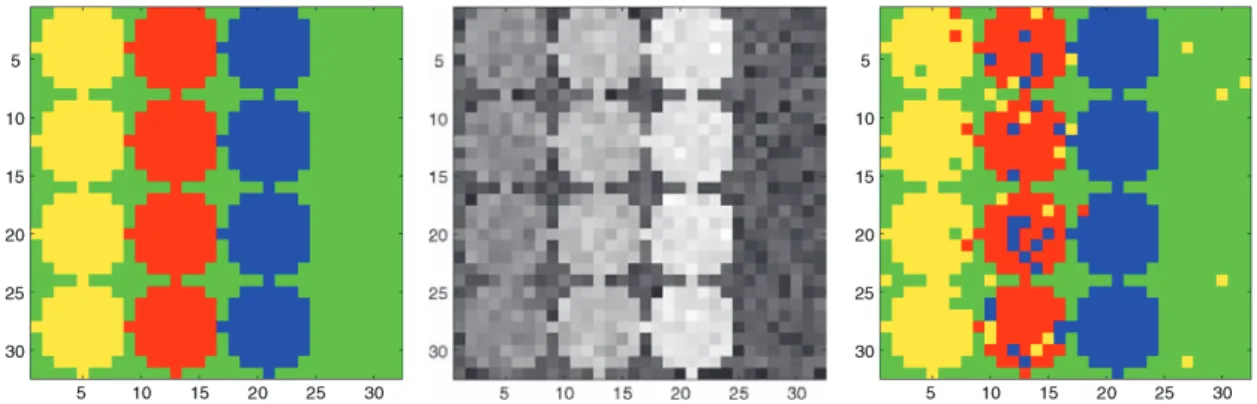
Figure 1. Example: Monoscale classification of pixels distributed in three “circle” classes of different intensities labeled by different colors against a background class (green). From left to right: “true” signal, “noisy” signal (gray-scaled), and pixel-scale clustering.

that are labeled according to underlying “circular” regions of different intensities (actually three different “circle” classes, one in each vertical region, against a background class). Figure1(center) displays the same image with additive noise. The purpose of a statistical classification method is to infer for each pixel in the noisy image the label of its class. In Figure1(right), a pixel-scale approach leads to a segmentation restricted to a spatial res-olution of the original pixels, with many false positives. A drawback of such monoscale approaches, as already noted by Bouman and Shapiro (1994), is that they use uniform pixel sizes across the image and therefore do not take into account local spatial variations, such as the characteristic shape and size of patches of various classes.

To capture the properties of each image region to be segmented, both large- and small-scale behaviors should be used to properly segment both large, homogeneous regions and detailed boundary regions. The method developed in this article is guided by such adaptive choices of spatial scale at each location. The main idea is that each potential class has its own spatial resolution within a scene. Our framework is based on a combination of re-cursive dyadic partitions and finite mixture models for clustering. To adaptively choose the locally best scale for clustering we use a multiscale method, based on recursive dyadic

par-titioning(RDP) of the image. RDP is now a widely used method in image processing (see, e.g., Donoho 1997or Kolaczyk, Ju, and Gopal2005). Starting our functional description of the pixel intensities on the finest resolution scale of a dyadic tree of square tiles (quads), we define a candidate model through a statistical likelihood, assuming statistical indepen-dence between signal measurements at different pixels. We then use a penalization method to encourage the aggregation of pixels when this is useful: similar regions of pixels that are likely to belong to the same cluster class are combined to a larger quad. A suitable penalty discourages trees with large numbers of splits, that is, too many unnecessarily small re-gions. Our RDP-based approach for combining adjacent spatial information replaces the correlation-model-based approaches such as “Hidden Markov” models that are frequent in the literature (see, e.g., Malfait and Roose1997or Choi and Baraniuk2001).

Finally, we point out that the originality of our work lies in the appropriate combination of the series of above-mentioned set of up-to-date statistical tools, which were developed in different (and mostly simpler) contexts in the literature. Our contribution is to select

and adapt them to our problem of segmenting images with functional pixel content, and to solve this problem efficiently without compromising theoretical validity.

The rest of the article is organized as follows. In the next section we describe our multi-scale setup in detail including our models for the pixel intensity curves and for the Gaussian mixture densities in the wavelet domain that are used for the clustering step. We give a flow-chart description of our complete algorithm before discussing certain details, in particular the dimensionality reduction of the set of wavelet estimators of the pixel intensity curves. To simplify the presentation, some part of the methodological and theoretical discussion of the properties of the aggregation estimator is relegated to an appendix document (ac-cessible via the journal’s webpage which also provides access to code and datasets of our numerical Section3). More details, including some theoretical results and their proofs, can be found in our accompanying discussion paper (Antoniadis, Bigot, and von Sachs2006). In particular, this article adapts a derivation of Kolaczyk, Ju, and Gopal (2005), to show that, from an asymptotic point of view, our method is able to correctly identify pixels be-longing to two different cluster classes.

In Section 3 we study the performance of our algorithm on simulated and real datasets, giving numerical comparisons with linear dimension-reduction schemes and with a monoscale scheme that show the usefulness of our RDP approach. We conclude with a discussion section and a sketch of possible extensions for future work.

2. MULTIRESOLUTION MODEL AND

METHODOLOGY ADOPTED

In this section we describe our model of functional pixel intensities, our overall method-ology including dimensionality reduction, and the spatial multiscale approach using recur-sive dyadic partitioning. We recall that the objective is to cluster the functional image content into relatively homogeneous spatial regions, each of which belongs to one of a (not necessarily known) number L of classes. The clustering is based on a functional charac-terization: pixels whose intensity curves are “similar” as multidimensional objects (of not too high dimensionality) should be put into the same cluster class.

Our algorithm is composed of several steps:

• wavelet denoising of functional pixel intensities combined with dimensionality re-duction,

• clustering using the fitted components of a Gaussian mixture model for each pixel intensity curve,

• spatial aggregation by penalized maximum likelihood that allows pixel-scale clusters to be recombined into larger regions (i.e., on coarser scales) of pixels belonging to the same cluster class.

Below we describe the development of the functional model for pixel intensities in the time and wavelet domains and our three-step algorithm. We underscore the need for a powerful initial dimensionality reduction step, so that clustering does not occur in a too

high-dimensional coefficient space. We develop the Gaussian mixture model that we use in the wavelet domain for our clustering step and give details of the EM algorithm used for clustering, including the choice of the number of clusters. Finally we give a fairly detailed description of our multiscale segmentation approach using recursive dyadic partitioning and complexity-penalized maximum likelihood.

2.1 MODEL DESCRIPTION

Model in the Functional Domain

Consider a finite spatial region of an image, say the unit square [0, 1]2. We have an r × r discretization of this region into pixels Ii, i = 1, . . . , N , N = r2. For each pixel I , let

xI(t ) denote its functional intensity at “time” t and let xI = (xI(t1), . . . , xI(tn))T denote

its “time” history, that is, the discretized sample path of the measurements for the pixel over “times” t ∈ {t1, t2, . . . , tn}, where n = 2Jn for some integer Jn. Note that here and

below we use “time” to denote the functional argument of the pixel intensity curves, even though this could just as well be frequency or something else.

For example, time-dependent intensity models might characterize temporal changes in blood flow or the decay of reactions to stimuli, whereas frequency-dependent models are used for magnetic resonance spectroscopy imaging (MRSI) for the detection of brain tu-mors.

We use the symbol c(i) to denote the class to which pixel i is assigned, and each of those c(i)takes on some value within the set of L pure classes, for simplicity labeled {1, . . . , L}. We assume that L < N . This leads to the following model for the intensity xi(t )of the ith

pixel:

xi(t )|{c(i) = ℓ} = fℓ(t ) + ε_iℓ(t ), t = t1, . . . , tn, n = 2J, 1 ≤ ℓ ≤ L, (2.1)

where fℓ is the underlying mean intensity for pixels in class ℓ, and ε_iℓ(t ) are zero-mean noises, 1 ≤ ℓ ≤ L. For generality, we allow for weak serial dependence in the noise processes assuming that the autocovariances of the noises are absolutely summable.

Model in the Wavelet Coefficient Domain

Starting from the nonparametric model (2.1) in the functional domain, our goal is to transform the problem into a coefficient domain to allow the densities of the resulting co-efficient vectors to be modeled via a parametric clustering approach. To this end we apply to each discretized curve xi, i = 1, . . . , N , an orthogonal discrete wavelet transformation

(DWT) over time t . This results in the following coefficient model. For pixel i, let wi be

the vector of the empirical wavelet coefficients {w_{j k}i } of xi at scales j = 0, . . . , J − 1, and

locations k = 0, . . . , 2j − 1. For each of these coefficients, let

w_{j k}i |{c(i) = ℓ} = θ_{j k}ℓ + ε_{j k}i , 1 ≤ ℓ ≤ L < N, (2.2) where we make an additional parametric assumption on the noise densities:

This gives rise to a Gaussian mixture model in the wavelet domain that lies at the heart of our maximum likelihood clustering approach. Specifically, we assume that

wi ∼ L

X

ℓ=1

πℓgℓ(θℓ, 6ℓ; w), i =1, . . . , N, (2.3)

where the parameters to be estimated are the prior mixture probabilities πℓ, the means θℓ,

and variances 6ℓof the Gaussian densities gℓ(·, ·)of class ℓ. Here, the means θℓdepend on

scale and location and the matrix 6ℓis diagonal with nonidentical variances σ_j,ℓ2 depending

on scale j , but not on location. This is in accordance with our model in the time domain which allows for serially correlated errors εi(t )with absolutely summable autocovariances

(see also Johnstone and Silverman 1997). For meaningful estimation of the above-given parameters, the number N of pixels has to be considerably larger than L.

2.2 OVERALLPROCEDURE

Given the above notation and model description in the functional (“time”) and wavelet coefficient domains, we now describe our complete algorithm.

1. Reduction of complexity/dimensionality reduction:

(a) Denoising step: For each pixel 1 ≤ i ≤ N , smooth its observed pixel intensity xi by applying nonlinear wavelet hard thresholding of the coefficients wi via

a universal threshold. Call these estimators ˆfi(t ), i = 1, . . . , N , t = t1, . . . , tn.

(b) Aggregation step: Take the union of all the wavelet coefficients of all the curves xi having survived thresholding in the first step.

Formally this can be described by an “aggregation estimator,” as in Bunea, Tsybakov, and Wegkamp (2007). We will use this to show that the optimal adap-tation of each of the individual estimators ˆfi(t ) to the possibly irregular

struc-ture of the pixel intensities over time, carries over to the spatially aggregated estimator ˆfλ(t ) =PNi=1λifˆi(t ). This estimator is a linear combination of the

ˆ

fi(t ) with certain optimal weights λi, i = 1, . . . , N (formally to be found by an

ℓ1-penalized least squares approach in the functional domain).

(c) Dimensionality reduction by truncating the aggregated estimator: Apply a Ney-man truncation thresholding test (Fan 1996) to the wavelet coefficients of the estimator ˆfλ(t )to further “sparsify” it. (We control the level of this multiple

hy-pothesis test using a false discovery rate approach; see Section2.3.) Collect the positions of the surviving wavelet coefficients. For this we use the classical or-dering in the wavelet domain, that is, {(j, k) : 0 ≤ j ≤ J − 1, k = 0, . . . , 2j− 1} = {(0, 0), (1, 0), (1, 1), (2, 0), . . .}). Construct new “dimension-reduced” estima-tors ˆxi(t )by taking the components of the empirical wavelet coefficient vectors

wiof xi(t )at these positions. The reduced, and common, dimensionality of these

estimators is typically two orders of magnitude smaller than the original curve lengths (i.e., the dimension of the vector wi).

In Section 2.3we comment in more detail on the aggregation and the final dimen-sionality reduction step.

2. Clustering on the pixel scale: Given the set of positions of reduced dimensional-ity, used for the coefficients of each curve i, we apply the EM algorithm of Law, Figueiredo, and Jain (2004) to estimate all parameters of model (2.2) and simultane-ously determine the number of clusters L that are present in the observed data. Here we work with the Gaussian mixture model (2.3). Some details on the algorithm can be found in Section2.4. To get back to the “pure class” model (2.2), for each pixel we assign the label with the highest estimated prior probability under EM.

3. Spatial multiscale approach: For the final spatial segmentation phase, to pass from monoscale (i.e., pixel scale) to multiscale, we use a penalized RDP approach to re-combine small pixel regions to large ones where appropriate. The fast tree-structured bottom-up algorithm compares the likelihood of each pixel collection on the finer scale with the one on the next coarser scale (by aggregating four neighboring fine-scale regions) and penalizes against too many elements in the resulting tree. Here, the estimation in model (2.3) and clustering are initially done at the finest RDP spa-tial resolution (the “pixel scale”), but note that, as detailed in Section 2.5, we use again EM in the complexity-penalized maximum likelihood algorithm to recalculate the mixing probabilities of the merged regions. To display our final results, we again use a majority vote to assign a coloring to each region.

We now give some useful insights into the various steps of our algorithm. Whenever we adapt ingredients of an existing method to our specific situation, we only give details of the adaptation, referring the reader to the cited literature for basic information about the method.

2.3 DIMENSIONALITYREDUCTION

It is essential to control the complexity of the estimation problem in step 1 as it is numerically impossible to estimate all occurring parameters of our model based on N intensity curves, for j = 0, . . . , J − 1, even after having applied a thresholding-based de-noising to their n = 2J wavelet coefficients. Hence, a dimensionality reduction is neces-sary: assuming that the curves do not behave “too differently” over time, we apply an “aggregation” approach (Bunea, Tsybakov, and Wegkamp2007) to find the optimal set of positions of empirical wavelet coefficients to preserve over all of the nonlinear wavelet estimators. We construct an aggregated estimator ˆfλ(t ) =PNi=1λifˆi(t ), and choose the

optimal λ = (λ1, . . . , λN)as in Bunea, Tsybakov, and Wegkamp (2007), by ℓ1-penalized

least squares in the functional domain. In practice, in the first step of dimensionality re-duction, we just take the union of the wavelet coefficients that survived hard thresholding using the universal threshold, in any of the individual curves. As this individual denoising method is known to be near-optimal with respect to minimal L2-risk for each individual

curve, it is interesting to ask whether this remains true for this new dimensionality reduc-tion procedure. By embedding this into the framework of “aggregareduc-tion,” we can indeed prove that this union remains a near-optimal denoising procedure when applied to the in-dividual curves. Some more details on this are to be found in the appendix document, with precise statements of our theoretical result and its proofs deferred to our discussion paper (Antoniadis, Bigot, and von Sachs2006).

However, whenever N is large, the aggregated wavelet denoiser may keep too many wavelet coefficients for each processed intensity curve. Hence, after aggregation, we have to increase the sparsity by using some truncation procedure that further reduces the num-ber of active coefficients before addressing the parametric estimation problem. In this final dimensionality reduction step we test whether, for each wavelet coefficient in the repre-sentative union, its expectation across the N intensity curves remains constant against the assumption that its expected behavior differs among curves. We give a short description of how to implement this interesting idea.

For a fixed wavelet-position k, denote the collection of coefficients from all curves at this position by w_ki, i = 1, . . . , N , and let d_ki = wi+1_k − wi_k, i = 1, . . . , N − 1, be the vec-tor of first-order differences of these coefficients. We observe that d_ki can be considered as a random sample from a Gaussian distribution N (µi_k, τ2), where µi_k= E(wi+1k − wik).

[Note that the variance τ2is closely related to the variance σ_j,ℓ2 of the wavelet coefficients w_{j k}i of model (2.2).] We will test the null hypothesis that the kth coefficient (even if it is im-portant for representing the curves) has no discriminative power for separating the classes, that is, the vector µ_k is identically equal to zero. Because the number of possible classes is small with respect to the total number of curves, most of the components of µ_k will be 0, and an appropriate procedure to test the eventual presence of nonzero components is to use the (hard) thresholding-based Neyman test of Fan (1996), with a test statistic essentially proportional to (a centered and standardized version of) PN_i=1(d_ki)2I (|d_ki| ≥ δH), and

as-ymptotically normal under the null. To control the multiplicity of this test, we use the false discovery rate (FDR) procedure as developed by Benjamini and Hochberg (1995). We re-mark that our procedure is completely justified by proposition 2.1 of Bunea, Wegkamp, and Auguste (2006).

We note that it is essential to apply this Neyman test after aggregation, that is, on the set of coefficients corresponding to a single wavelet threshold estimator. This is in order to be able to correctly apply the FDR procedure: if Fan’s procedure on dimensionality reduction were applied to each curve individually, the correlations of estimated wavelet coefficients across all curves would need to be modeled to apply an (accordingly modified) FDR procedure.

The Appendix section of the accompanying discussion paper (Antoniadis, Bigot, and von Sachs2006) gives more details and theoretical results on aggregation and the optimiza-tion of the aggregaoptimiza-tion risk, as well as some details of the truncaoptimiza-tion test procedure used for final dimensionality reduction. We also give there a small theoretical result on correct clustering within the “horizon model” framework of Donoho (1999), a two-label model with an arbitrary Lipschitz-frontier between the two regions. Note that these techniques were already suggested by Korostelev and Tsybakov (1993) in their “model of bound-ary fragments” to prove near-optimal minimax results for classification. To be able to use these techniques here we have to make an additional approximation by assuming indepen-dence (noting that the series of operations performed on the initial set of hypothetically uncorrelated wavelet coefficients does not allow to maintain this assumption to be exactly fulfilled).

2.4 THEEM ALGORITHMUSED FOR CLUSTERING

We use the refined EM algorithm of Law, Figueiredo, and Jain (2004) to estimate the parameters of the Gaussian mixture model (2.3). This algorithm is distinguished from other existing methods by the fact that it automatically estimates the number L of cluster classes, in a way that proves to be far less sensitive to the high dimensionality of the problem than, for example, the approach by Sugar and James (2003).

To select L adaptively, Law, Figueiredo, and Jain (2004, sec. 3.3) used an approach based on the MML (minimum message length) criterion, given an upper bound Lmax on

the number of classes. This approach is closely related to MDL (minimum description length), adding to the negative log-likelihood a series of terms that “penalize” against the number of model parameters. For more details of this algorithm see our discussion paper (Antoniadis, Bigot, and von Sachs 2006) and the original paper of Law, Figueiredo, and Jain (2004).

2.5 RECURSIVEDYADICPARTITIONING AND COMPLEXITY-PENALIZED

MAXIMUMLIKELIHOOD

Using recursive dyadic partitioning (RDP) to model a multiscale hierarchy of spatial scales of an image (the unit square [0, 1]2, say) by means of an inhomogeneously pruned dyadic quad-tree is now a well-established approach in the literature. For a complete for-mal description we refer to Kolaczyk, Ju, and Gopal (2005), but see also Donoho (1997). Here, we recall the general ideas, before combining them with our specific setup of max-imum likelihood estimation. We specify the components of our RDP model compared to the more complex one of Kolaczyk (which is not only multiscale but also multigranular). To briefly develop the formal analogies, let a model M in the set M of all possible models on the quad-tree be a tuple made up of two components: (i) a complete RDP (i.e., a col-lection of disjoint quadratic dyadic regions R, not necessarily of the same size, the union of which covers exactly the original image [0, 1]2); (ii) a density fM(wi|c(R)) assigned

to each region R from which the pixel intensity coefficient wi for each pixel Ii ∈ R is

sampled independently, where c(R) ∈ {1, . . . , L} is the class label associated to region R. Using model (2.3) for the Gaussian mixture densities on the pixel scale, the likelihood for coefficient vector wi on region Ri with its class label ci= c(Ri)is now given by

fM(wi|ci) = L

X

ℓ=1

πℓ(Ri)gℓ(θℓ, 6ℓ; wi). (2.4)

In words, we have a model with regions Ri and mixtures with mixture probabilities πℓ(Ri)

for each of the classes 1 ≤ ℓ ≤ L, assigned to all the pixels in the region Ri. We recall that

the regions at the pixel scale are assumed to be homogeneous in one of the “pure” classes {1, . . . , L}.

Estimation is done again using the EM algorithm already used for the Gaussian mixture densities on the pixel scale, and hence the estimated likelihood for coefficient vector wi is

ˆ fM(wi|ci) = L X ℓ=1 ˆ πℓ(Ri) ˆgℓ(wi), (2.5)

noting that ˆgℓ(wi) := g( ˆθ_ℓ(i), ˆ6_ℓ(i); wi)denotes the Gaussian likelihood of coefficient wi

with estimated mean ˆθ_ℓ(i)and estimated variance ˆ6(i)_ℓ .

Complexity-Penalized Maximum Likelihood

The tree-based algorithm for complexity-penalized maximum likelihood, using the (es-timated) likelihood (2.5), is a fully grown-pruned back standard algorithm based on an additive cost function. We briefly explain it now. At the coarsest spatial scale the entire image is treated as a single “pixel,” and at consecutive finer scales, the image can be fur-ther split into four square quads, until the finest scale of an individual pixel is reached. What is important is the possibility to allow the quad size to vary across the image, instead of working with only monoscale representations (i.e., with uniform quad sizes). To find this best-adapted spatially heterogeneous image representation (i.e., model), the complete tree grown down to pixel scale needs to be pruned back using a penalized goodness-of-fit criterion through the above-given statistical likelihood, assuming statistical independence between signal measurements among pixels. Penalization is used to encourage aggrega-tion of pixels to larger regions whenever a parent region has larger complexity-penalized maximum likelihood than the union of its four descendant children regions.

More formally, we will identify the best model in M by maximizing a complexity-penalized likelihood function in the wavelet coefficient domain

b

M =arg max

M∈M{ℓ(w|M) − 2 pen(M)}. (2.6)

Here, using the individual likelihood ˆfM(wi|ci)from (2.5),

ℓ(w|M) = Y

{i : Ii∈R∼M}

ˆ

fM(wi|ci),

where the notation R ∼ M is used to denote all quad regions R which make up the complete RDP associated to model M.

Optimization can be done using a standard bottom-up tree pruning algorithm: beginning at the finest spatial resolution, select the class c for each pixel Ii with the largest

log-likelihood. Next, for each quad of four pixels, compare the complexity-penalized likelihood of two submodels: (i) the union of the four most likely single pixel models with its penalty for a single spatial split (i.e., splitting the quad into four pixels); (ii) the single model for the set of four pixels that is most likely among all allowable c ∈ {1, . . . , L} with its smaller penalty. Continuing this in a recursive fashion leads to model bM.

The choice of the appropriate penalty in (2.6) is motivated from general ideas of model selection following the ideas of Birgé and Massart (1998). More specifically, as one pos-sibility for a penalty working in practice we propose to choose pen(M) = β|M|, which results from an adaptation of the approach of Lavielle (2005). We give some more details about this choice in our appendix document, including a proposition that suggests the fol-lowing graphical method for selecting from the data the parameter β and the correspond-ing dimension m = |M|: examine how the negative log-likelihood −ℓ(w(·)|m) decreases as a function of increasing model dimension m, and select the dimension ˆmfor which the neg-ative log-likelihood ceases to decrease significantly. The above procedure is very similar to

the nonlinear L-curve regularization method used for determining a proper regularization parameter in penalized nonlinear least squares problems (see Gulliksson and Wadin1998). In our context, the L-curve is defined as the curve (−ℓ(x(·)|m(β)); m(β))β≥0and defines a

strictly decreasing convex function with a derivative with respect to m(β) equal to −β. The L-curve has usually a distinct corner, defined as the point where the L-curve has its greatest curvature and corresponding in our case to the point β where the negative log-likelihood ceases to decrease. In Section3, along with our numerical examples, we describe a more refined procedure how to find an “optimal” β and the corresponding “optimal” dimension

ˆ m(β).

Note that this RDP approach, though using the assumption of independency over pix-els, allows to recombine pixels in the same label class and hence is an alternative to more classical approaches which work with correlation models over neighboring pixels. To re-spond to the possible criticism of being restricted with RDP to spatially only dyadically representable regions, we mention that Kolaczyk, Ju, and Gopal (2005) had a translation-invariant (TI) version of this two-dimensional RDP which was able to approximate more general regions of spatial homogeneity. In Section3we will use such a TI version of the RDP for spatial recombination (whereas we continue to use an orthogonal wavelet trans-form for the temporal dimensionality reduction).

3. NUMERICAL EXAMPLES

In this section we present some results of our methods on simulated and on real data. 3.1 SIMULATEDEXAMPLES

We first use a synthetic example for which the true classes are known to illustrate the performance of our approach and to compare it with a simpler technique for selecting the wavelet coefficients. The example consists of an N × N simulated image containing a 4 × 3 grid of circles that correspond to active regions, with N = 32 and circles of diameter 8 pix-els (see Figure2). We first consider the case where each active region contains a single sig-nal. There are three distinct signals in the image, corresponding to the three columns from

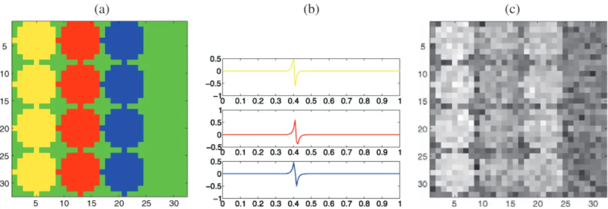
(a) (b) (c)

Figure 2. Circles images: (a) true classes corresponding to 12 active regions in three columns of four rows with N =32, (b) signals in each active region (yellow, red, and blue pixels), (c) an example of a temporal slice with SNR = 3.

Table 1. Comparison between our nonlinear scheme and three linear methods, giving the number of times the EM algorithm finds the true number of classes (bold numbers) and the misclassification rates (numbers in brackets) over the 100 simulations. Note that misclassification rates are averages over successful simulations, that is, those for which the procedure correctly identifies the number of regions (L = 4).

SNR 3 2 1.5

Nonlinear selection 80 (0.0408) 72 (0.0760) 86 (0.1275) Linear selection j = 4 87 (0.1700) 50 (0.3289) 16 (0.4164) Linear selection j = 5 1 (0.0029) 7 (0.0188) 15 (0.2419) Linear selection j = 6 26 (0.0000) 27 (0.0003) 6 (0.0015)

left to right. The remaining pixels (in green) contain no signal and can therefore be con-sidered to belong to a pure noise class. The three signals are generated using a difference of exponentials fℓ(t ) = a + b(e−|t−uℓ,1|/Tℓ,1− e−|t−uℓ,2|/Tℓ,2), ℓ =1, . . . , 3. The twelve

ac-tive regions and the three signals are shown in Figure2. The values of uℓ,1 and Tℓ,1 have

been chosen to give similar signals of short time support which makes discriminating be-tween them difficult with linear methods. We use a uniform sampling of the signals over the interval [0, 1] with n = 128. For three different values of the signal-to-noise ratio, we created 100 simulated images by adding Gaussian white noise. A typical temporal slice is displayed in Figure2(c).

First, we compare our nonlinear approach for selecting the significant wavelet coeffi-cients (dimensionality reduction step using thresholding, aggregation, and Neyman trun-cation) with a linear approach that only keeps the first 2j wavelet coefficients. For both approaches (either nonlinear or linear) we then use the EM algorithm of Law, Figueiredo, and Jain (2004) to estimate the number of classes and to cluster the pixels. In our example the true number of classes is L = 4. In Table1we report the results for a signal-to-noise ratio (SNR) equal to 3, 2, and 1.5, and for j = 4, 5, 6. For each method we indicate the number of times the EM algorithm finds the true number of classes, and for these cases we calculate the number of misclassified pixels. In Table1we give the misclassification rates of each method over the 100 simulations. Our nonlinear approach clearly outperforms the three linear methods for the estimation of the true number of classes. Its misclassification rates are also much lower than with j = 4. For j = 5, 6, if the linear approach finds the true number of clusters, it may also obtain better classification results. Note, however, that for j = 5, 6 and all values of the SNR, the estimation of the true number of classes over the 100 simulations is very poor compared to the results obtained with our nonlinear scheme.

Note that the EM algorithm of Law, Figueiredo, and Jain (2004) is initialized randomly, which may in different runs give different results for the estimated number of classes and the final pixel-scale clustering. Even for the same estimated number of classes, the cluster-ing at the pixel scale may be very different, and hence in practice it is highly recommended to run the algorithm several times. This problem is shared by any EM algorithm and not specific to our setup here. Nevertheless, our simulations clearly show the benefits of our nonlinear scheme for clustering the image at the pixel scale.

Next, we present some simulations to show the usefulness of the translation-invariant (TI) RDP step relative to a simple classification at the pixel scale. For this we use a mixture

Table 2. Prior mixture probabilities πℓ, ℓ = 1, . . . , 4, for each class of the circles image.

π_ℓ ℓ =1 ℓ =2 ℓ =3 ℓ =4 Yellow class 0.85 0.05 0.05 0.05 Red class 0.05 0.85 0.05 0.05 Blue class 0.05 0.05 0.85 0.05 Green class (pure noise) 0.025 0.025 0.025 0.925

model to generate noisy functional images. In each of the regions displayed in Figure2(a), a noisy signal of length n = 128 is generated according to the following Gaussian mixture model: xi(t ) = 4 X ℓ=1 π_ℓifℓ(t ) + εi(t ), i =1, . . . , N,

where f4= 0 (pure noise class) and the εi(t )’s are iid normal variables with zero mean

and variance σ2 (same variance for all pixels). Note that the prior mixture probabilities π_ℓi = π_ℓc(i) depend on the class and are given in Table2.

Again we generate 100 noisy images for three different values of the signal-to-noise ratio. For each image, we use our nonlinear approach to select the significant wavelet co-efficients and the EM algorithm of Law, Figueiredo, and Jain (2004) to find the number of classes and the parameters of the Gaussian mixture model. A typical example of clustering for SNR = 3 for this mixture model is given in Figure3(a). One can see that some pixels are misclassified and that the classes do not form spatially homogeneous regions. To

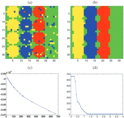
im-(a) (b)

(c) (d)

Figure 3. Circle image with a mixture model for each class: (a) clustering at the pixel scale, (b) final clustering with a TI-RDP step, (c) L-curve, (d) curve (β, m(β)).

prove the classification at the pixel scale, we use the penalized RDP algorithm. To choose the parameter β in the complexity-penalized likelihood criterion, we apply the following automatic method motivated by the L-curve regularization approach described in Section 2.5. This method for finding the “optimal” β and the corresponding “optimal” dimension

ˆ

m(β)is based on the “slope heuristic” idea. The contrast (i.e., the penalized log-likelihood) associated to a RDP is the sum of two terms: the likelihood term represents approximation error within the associated clustering, that is, bias, and the penalty term represents the com-plexity of the model and can therefore be interpreted as a variance term. The idea of the heuristic is that when a model is high-dimensional, the associated bias is close to zero, and so the contrast of the RDP is essentially an estimate of the variance of the model which is directly related to the size m of the RDP. Hence, for large m, the negative log-likelihood should become a linear function of m. The choice of the dimension ˆmbeyond which the negative log-likelihood becomes linear is left to the user. The choice of ˆmcan be based on visual inspection of the L-curve (−ℓ, m(β)), and is obtained by selecting the dimension m for which the negative likelihood ceases to decrease significantly and becomes linear. To choose ˆm, one can also plot the curve (β, m(β)) and search for the parameter β associated to the first significant jump in this curve. Once we have chosen the appropriate dimension

ˆ

m, the basic principle is to fit a linear regression of −ℓ with respect to m for m ≥ ˆm. If we denote by ˆαthe estimated regression coefficient, then as suggested by Birgé and Mas-sart (2001), an appropriate estimator for β is given by ˆβ = κ ˆα where κ is a constant close to 2 (in practice we take κ = 2).

For the example in Figure 3(a), ˆβ is estimated to be 1.5736 using the slope heuristic, the final segmentation is given in Figure 3(b), and we display the L-curve (−ℓ, m(β)) in Figure 3(c) and the curve (β, m(β)) in Figure 3(d). In our simulations, the selected dimension ˆmbeyond which the L-curve is considered as a linear function is 150. In this example one can see that the RDP step significantly improves the misclassification rate. In particular, the classes are now spatially homogeneous. However, the TI version of RDP tends to oversmooth the edges of the region, which explains why the estimated active regions in Figure3(b) appear to extend beyond those of the original image in Figure2(a).

In Table 3 we compare the misclassification rates of the pixel-scale and RDP ap-proaches. Again, we compute the misclassification rate only for the cases where the EM algorithm finds the true number of classes. These results show that the final segmentation with penalized RDP improves the misclassification rate (particularly for situations of still higher signal-to-noise ratio, as experiments not reported here have confirmed). The final step yields homogeneous spatial regions but some pixels at the boundaries of the circles are

Table 3. Comparison of the misclassification rate over 100 simulations between clustering at the pixel scale and clustering using the TI-RDP method. The number of successful identifications of the number of classes by EM is around 80 as for those from the simulation in Table1.

SNR 3 2 1.5

Clustering at the pixel scale 0.2285 0.2258 0.2059 Clustering with the RDP 0.2063 0.2180 0.2010

misclassified owing to oversmoothing effects as can be seen in Figure3(b). This explains why the misclassification rates do not decrease very much for our chosen simulation setup with N = 32. We believe that increasing the spatial resolution would allow more significant improvements to be observed; however, we refrained from performing a time-consuming simulation study here. Note that if the non-TI version of RDP is used, the algorithm ap-proximates the circles with large squares, resulting in poor boundary estimation, and hence an increased misclassification rate.

Our second example is the simulated image of Whitcher et al. (2005), with size parame-ters N = 64 and n = 128. For convenience we give a short description of this dataset. The segmentation of the image can be found in Whitcher et al. (2005) which partly motivated our own work, and which is a typical example of a functional pixel-scale approach based on wavelet methods. These authors examined MRI time series experiments (e.g., brain responses to pharmacological stimuli) that produced statistical data in two or three spatial dimensions that evolved over time. Their nonparametric approach groups pixels (or voxels) with similar time courses based on the discrete wavelet transform representation of each time course, thus giving localized pixel information over time and spatial (mono-) scale. Similarly to our “Circles” image, the simulated signals were generated using a difference of exponentials S(t) = a + b(e−t/To _{− e}−t/Ti_{), with different values of T}

i and To, in 12

active regions in three columns of four rows (with the fourth column corresponding to an inactive region). The maximum signal amplitudes were normalized relative to the standard deviation of the additive Gaussian white noise such that the contrast-to-noise ratio in each row was 6, 4, 2, and 1. The spatial form of the active regions was a circular region of di-ameter 8 pixels, containing maximum intensity at each active region. This was surrounded by a Gaussian taper to zero within a square of 12 pixels, this providing a locally varying contrast-to-noise ratio.

To give an idea of the signals that we have to cluster we display a typical temporal slice and noisy time curves corresponding to two pixels in Figure4.

Because of the Gaussian tapering, and given the fact that different standard deviations are used for the noise in each row, the “true classes” are not very well defined for this image. Hence, rather than trying to decide whether our algorithm finds the true classes, we compare the clustering obtained with our approach with the segmentation obtained

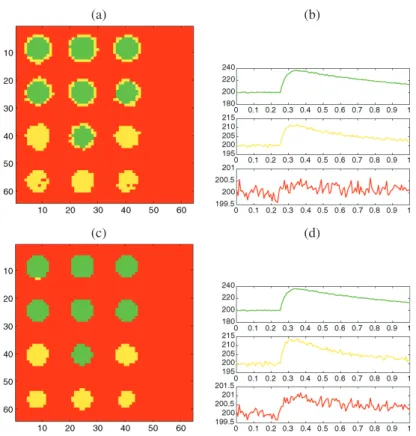
(a) (b)

(a) (b)

(c) (d)

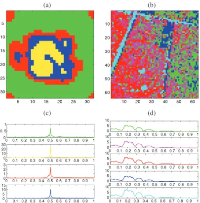
Figure 5. Whitcher image: (a) clustering and (b) average time curves for each cluster at the pixel scale, (c) clus-tering and (d) average time curves for each cluster with a TI-RDP step.

by Whitcher et al. (2005). Using the dimensionality reduction step, as described in Sec-tion2.3, that is, truncating the union of the wavelet coefficients of all pixel intensity curves that survived the initial hard thresholding, we finally retain ˆk = 10 wavelet coefficients for the clustering steps. After applying the EM algorithm of Law, Figueiredo, and Jain (2004), the number of estimated classes is ˆL =3. The corresponding clustering at the pixel scale is shown in Figure 5. To give an idea of how well the algorithm clusters the pixels, the “average” time curves from the groups determined by the procedure are also displayed. Finally we apply the slope heuristic as described previously, to choose the parameter β of the complexity-penalized likelihood criterion and select the best RDP. The selected dimen-sion ˆmbeyond which the L-curve is considered to be linear is 193 and the corresponding estimate of β is 1.8870. The TI version of RDP with these parameters is shown in Figure5 together with average time curves from each cluster. Our algorithm clearly identifies the twelve active regions and the background noise. Whitcher et al. (2005) allowed the number of clusters to increase to L = 6 because taking L = 3 gives very poor identification of the active regions with their method. Note that in Whitcher et al. (2005), the clusters are iden-tified via a linear selection of the wavelet coefficients combined with standard EM and the choice of the number of clusters is based on the method of Sugar and James (2003). Our approach is somewhat different as we use nonlinear selection of the wavelet coefficients and the EM algorithm of Law, Figueiredo, and Jain (2004) to choose ˆL. In Whitcher et al. (2005), the twelve active regions are divided into four clusters whereas the background noise is partitioned into two groups. Both approaches essentially identify the same active regions. The rings of activation where the Gaussian kernel is used to taper the SNR of the

active regions were detected in Whitcher et al. (2005) and by our approach with cluster-ing at the pixel scale. Spatial clustercluster-ing with TI-RDP eliminates these rcluster-ings of activation and yields spatially homogeneous regions. The average time curves for each active cluster (the yellow and green signals in Figure 5) show that our algorithm partitions the pixels of the yellow and green regions respectively according to their rapid and slower activa-tion curves. The same kind of division between the four active clusters is also observed in Whitcher et al. (2005).

3.2 REALEXAMPLES

Now, we consider the following examples based on real data:

• the MRSI image (see description below): the size parameters are N = 32 and n =4,096.

• the ONERA image: a multiband satellite image of remote sensing measurements in various spectral bands of an area that contains roads, forests, vegetation, lakes, and fields. The size parameters are N = 64, with n = 128 frequencies.

As the MRSI application is the main motivation for our work, we will describe the magnetic resonance spectra images in some detail. MRSI for detection of brain tumors is an example of data with frequency-dependent pixel intensity curves where the maximum number of classes Lmaxis actually known. Tumor tissues are classified according to

(usu-ally three) different types of tumor and (frequently five) different grades of malignancy, making up the pure reference classes for our clustering problem (see Szabo De-Edelenyi et al. 2000). As an alternative to invasive brain biopsy for diagnosis, MRSI has become one of the most important noninvasive diagnostic aids in clinical decision making, mostly because of the good visibility of soft tissue structures to assess location and size of the tumor; see, for example, Meyerand et al. (1999).

For the above two examples, Figures 6 and 7 display typical temporal slices (a) and noisy curves (b) corresponding to two pixels to give an idea of the signals that we have to cluster.

(a) (b) (c)

Figure 6. MRSI image: (a) a temporal slice, (b) noisy curves associated to two pixels, (c) sorted test statistics T₁H, . . . , T_kH

(a) (b) (c)

Figure 7. ONERA image: (a) a temporal slice, (b) noisy curves associated to two pixels, (c) sorted test statistics T₁H, . . . , T_kH

maxin absolute value and decreasing order.

For each image, we first applied wavelet hard tresholding using a universal threshold and a MAD estimator on the finest scale to estimate the variance of the wavelet coefficients. Then we applied dimensionality reduction by truncation as described in Section 2.3 on the union of the wavelet coefficients that survived the first hard thresholding. Figures 6 and7(c) plot the first 100 statistics T₁H, . . . , T_kH_max based on Neyman’s procedure (sorted in absolute value and decreasing order).

As explained by Bunea, Wegkamp, and Auguste (2006), the very large first values of these sorted statistics correspond to the null hypotheses to be rejected and thus to the most discriminative wavelet coefficients to separate the classes. In the FDR procedure, one has to choose a user-specified value q ∈ (0, 1) which controls the ratio of the expected number of false rejections to the total number of rejections. Note that in Bunea, Wegkamp, and Auguste (2006) no data-dependent choice for this parameter is proposed. For the two im-ages, we chose q = 0.05 but this is obviously not an optimal tuning for this parameter (the same value was used for the simulations with the Circles and Whitcher images). The am-plitude of the statistics is very different for the two images. Actually, the magnitude of the largest T_iH’s is proportional to the signal-to-noise (SNR) ratio of the curves that we have to cluster. For the MRSI image, the SNR is very high and the amplitude of the largest test statistics is therefore extremely high (≥107). As a comparison, for the Whitcher image, the SNR is very low (see Figure4(b)) and the amplitude of the largest test statistics is therefore extremely low (≈60) as compared to the values of the test statistics for the MRSI image.

If we apply the FDR procedure with q = 0.05 to each of the two images, the number ˆk of selected wavelet coefficients is 2629 for the MRSI image and 66 for the ONERA im-age. For the MRSI image, the selected ˆk is obviously too large. Hence, based on visual inspection of the decay of the test statistics in Figure6(c), we prefer to choose ˆk = 50. The issue of choosing ˆk automatically is not that obvious. On the one hand we tried to retain the formality of FDR and the use of q, but on the other hand one must admit that it is not always the right way to choose ˆk. Depending on the amplitude of the T_kH’s, it might be more informative to directly choose ˆk by a visual inspection of the curve of the sorted test statistics.

After applying the EM algorithm of Law, Figueiredo, and Jain (2004), we obtain the fol-lowing estimate ˆLfor the number of classes: 4 for the MRSI image and 5 for the ONERA

(a) (b)

(c) (d)

Figure 8. Clustering at the pixel scale for the (a) MRSI image, (b) ONERA image. Average time curves for each cluster for the (c) MRSI image, (d) ONERA image.

image. The corresponding clusterings at the pixel scale are given in Figure8. To give an idea of how well the algorithm is clustering the pixels, the “average” time curves from the groups determined by the procedure are also displayed.

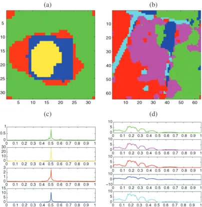
Finally we apply the slope heuristic to choose the parameter β that gives the best RDP. The selected dimension ˆm beyond which the L-curve is considered as a linear function is 130 for the MRSI image and 700 for the ONERA image, and based on the slope heuristic we obtain the following estimates: ˆβ =1.6908 for the MRSI image, and ˆβ =1.8199 for the ONERA image. The TI versions of RDP with these parameters are shown in Figure9. Average time curves from the groups determined by the procedure are also displayed.

In summary, we observe that the ONERA example greatly benefits from the final RDP step and that it is even highly necessary. We believe that the MRSI image also gains clar-ity. Remember that the results at the pixel level give many spatially dispersed pixels. For this example this does not make much sense because we are trying to recover a specific segmentation of the tissues that the tumor has gradually evaded (regions with a different severity). For the reader’s convenience the journal’s webpage provides access to our code and the data of the MRSI image such that all figures and tables of this section can be reproduced.

4. CONCLUSION

Our approach is certainly not the only possible one for clustering images with functional pixel intensities. However, we believe that it is a very appropriate nonparametric

possibil-(a) (b)

(c) (d)

Figure 9. TI RDP for the (a) MRSI image, (b) ONERA image. Average time curves for each cluster for the (c) MRSI image, (d) ONERA image.

ity that simultaneously addresses the problems of high dimensionality (spatial times func-tional dimension) and the drawbacks of working with a pixel-scale approach. By way of comparison we considered a variety of algorithms that turned out to be very sensitive to the high dimensionality of the problem, for example, the work by Sugar and James (2003) for finding the number of clusters, and the information criterion methods of Biernacki, Celeux, and Govaert (2000). Similarly, approaches based on modeling spatial correlation between pixels, such as kriging, suffer from the high spatial dimensionality (one possibility here would be to use reversible MCMC like Vannucci, Sha, and Brown (2005) but this is very time-consuming).

Wavelets seem to offer clear advantages in addressing the functional dimension of the problem, but as our various numerical examples have shown, there is a need to use

multi-scalespatial approaches rather than monoscale ones such as Whitcher et al. (2005). For the spatial multiscale modeling, in this article we used an approach based on RDP motivated from the work by Kolaczyk, Ju, and Gopal (2005), but one could also con-sider other spatial models, for example, Markov fields. Comparing our method with mul-tiscale hidden Markov approaches, such as the work of Malfait and Roose (1997) or Choi and Baraniuk (2001), we note that both articles dealt with supervised classifica-tion/segmentation. However, it would be interesting to replace the complexity-penalized RDP step of our approach with a wavelet-domain hidden Markov tree, to see how the latter would perform in combination with our unsupervised clustering step (after our nonpara-metric dimensionality reduction step).

Other comparisons could include the approach of Berlinet, Biau, and Rouvière (2008) which is again on supervised classification. However, we found that a criterion based on or-dering the energy in the domain of squared coefficients, as in principal components analy-sis, does not necessarily have good discriminating power and in general would not work in practice. See also the example in Figure 3 of the paper by Law, Figueiredo, and Jain (2004).

ACKNOWLEDGMENTS

We thank the associate editor and the two referees for their constructive comments which have helped to improve the presentation of the material of our article. We are particularly indebted to Bill Triggs for his careful reading of the manuscript to be put in a style suitable for publication in JCGS. Jérémie Bigot and Rainer von Sachs thank Anestis Antoniadis for his continuing hospitality during several visits at UJF in Grenoble. Anestis Antoniadis thanks Rainer von Sachs for excellent hospitality while visiting the Institute of Statistics, UCL to carry out this work. Fruitful discussions with Eric Kolaczyk, Hernando Ombao, Marina Vannucci, and Brandon Whitcher are gratefully acknowledged. An earlier version of this work was presented at the 2006 Graybill Con-ference on “Multiscale Methods and Statistics” at CSU, Fort Collins. Financial support from the IAP research network Nr. P5/24 of the Belgian government (Belgian Science Policy) is gratefully acknowledged.

REFERENCES

Antoniadis, A., Bigot, J., and von Sachs, R. (2006), “A Multiscale Approach for Statistical Characterization of Functional Images,” Discussion Paper 0623, de l’Institut de Statistique, Université catholique de Louvain, Louvain-la-Neuve. Available athttp:// www.stat.ucl.ac.be/ ISpub/ dp/ 2006/ dp0623.pdf.

Benjamini, Y., and Hochberg, Y. (1995), “Controlling the False Discovery Rate: A Practical and Powerful Ap-proach to Multiple Hypothesis Testing,” Journal of the Royal Statistical Society, Ser. B, 57, 289–300. Berlinet, A., Biau, G., and Rouvière, L. (2008), “Functional Supervised Classification With Wavelets,” Annales

de l’ISUP, 52, 61–80.

Biernacki, C., Celeux, G., and Govaert, G. (2000), “Assessing a Mixture Model for Clustering With the Integrated Completed Likelihood,” IEEE Transactions PAMI, 22 (7), 719–725.

Birgé, L., and Massart, P. (1998), “Minimum Contrast Estimator on Sieves: Exponential Bounds and Rates of Convergence,” Bernoulli, 4, 329–375.

(2001), “A Generalized Cp Criterion for Gaussian Model Selection,” Technical Report 647, Universités de Paris 6 et Paris 7, France.

Bouman, C., and Shapiro, M. (1994), “A Multiscale Random Field Model for Bayesian Image Segmentation,”

IEEE Transactions on Image Processing, 3 (2), 162–177.

Bunea, F., Tsybakov, A., and Wegkamp, M. (2007), “Aggregation for Gaussian Regression,” Annals of Statistics, 35, 1674–1697.

Bunea, F., Wegkamp, M., and Auguste, A. (2006), “Consistent Variable Selection in High Dimensional Regres-sion via Multiple Testing,” Journal of Statistical Planning and Inference, 136, 4349–4364.

Choi, H., and Baraniuk, R. G. (2001), “Multiscale Image Segmentation Using Wavelet-Domain Hidden Markov Models,” IEEE Transactions on Image Processing, 10 (9), 1309–1321.

Donoho, D. L. (1997), “Dyadic Cart and Ortho-Bases: A Connection,” Annals of Statistics, 25, 1870–1911. (1999), “Wedgelets: Nearly-Minimax Estimation of Edges,” Annals of Statistics, 27, 859–897. Fan, J. (1996), “Test of Significance Based on Wavelet Thresholding and Neyman’s Truncation,” Journal of the

Gulliksson, M., and Wadin, P.-A. (1998), “Analyzing the Nonlinear L-Curve,” technical report, Dept. of Comput-ing Science, University of Umea, Sweden.

Johnstone, I. M., and Silverman, B. (1997), “Wavelet Threshold Estimators for Data With Correlated Noise,”

Journal of the Royal Statistical Society, Ser. B, 59, 319–351.

Kolaczyk, E., Ju, J., and Gopal, S. (2005), “Multiscale Multigranular Statistical Image Segmentation,” Journal of

the American Statistical Association, 472, 1358–1369.

Korostelev, A. P., and Tsybakov, A. (1993), Minimax Theory of Image Reconstruction, New York: Springer. Lavielle, M. (2005), “Using Penalized Contrasts for the Change-Point Problem,” Signal Processing, 85 (8), 1501–

1510.

Law, M., Figueiredo, M., and Jain, A. (2004), “Simultaneous Feature Selection and Clustering Using Mixture Models,” IEEE Transactions PAMI, 26 (9), 1154–1166.

Malfait, M., and Roose, D. (1997), “Wavelet-Based Image De-Noising Using a Markov Random Field a priori Model,” IEEE Transactions on Image Processing, 6, 549–565.

Meyerand, M. E., Pipas, J. M., Mamourian, A., Tosteson, T. D., and Dunn, J. F. (1999), “Classification of Biopsy-Confirmed Brain Tumors Using Single-Voxel MR Spectroscopy,” American Journal of Neuroradiology, 20, 117–123.

Sugar, C., and James, G. (2003), “Finding the Number of Clusters in a Data Set: An Information Theoretic Approach,” Journal of the American Statistical Association, 98, 750–763.

Szabo De-Edelenyi, F., Rubin, C., Esteve, F., Grand, S., Decorps, M., Lefournier, V., Le-Bas, J. F., and Remy, C. (2000), “A New Approach for Analyzing Proton Magnetic Resonance Spectroscopic Images of Brain Tu-mors,” Nature-Medicine, 6, 1287–1289.

Vannucci, M., Sha, N., and Brown, P. J. (2005), “NIR and Mass Spectra Classification: Bayesian Methods for Wavelet-Based Feature Selection,” Chemometrics and Intelligent Laboratory Systems, 77, 139–148. Whitcher, B., Schwarz, A. J., Barjat, H., Smart, S. C., Grundy, R. I., and James, M. F. (2005). “Wavelet-Based

Cluster Analysis: Data-Driven Grouping of Voxel Time-Courses With Application to Perfusion-Weighted and Pharmacological MRI of the Rat Brain,” Neuroimage, 24 (2), 281–295.