To cite this document:
Ponzoni Carvalho Chanel, Caroline and Farges, Jean-Loup and
Teichteil-Königsbuch, Florent and Infantes, Guillaume POMDP solving: what rewards
do you really expect at execution? (2010) In: The 5th Starting Artificial Intelligence
Researche Symposium, 16 August 2010 - 20 August 2010 (Lisbon, Portugal).
O
pen
A
rchive
T
oulouse
A
rchive
O
uverte (
OATAO
)
OATAO is an open access repository that collects the work of Toulouse researchers and
makes it freely available over the web where possible.
This is an author-deposited version published in:
http://oatao.univ-toulouse.fr/
Eprints ID: 11446
Any correspondence concerning this service should be sent to the repository
administrator:
[email protected]
POMDP solving: what rewards do you
really expect at execution?
Caroline Ponzoni Carvalho CHANELa,b Jean-Loup FARGESa and
Florent TEICHTEIL-KÖNIGSBUCHa and Guillaume INFANTESa
aONERA - Office National d’Etudes et de Recherches Aérospatiales,
Toulouse, France. Email: [email protected] b
ISAE - Institut Supérieur de l’Aéronautique et de l’Espace Abstract.Partially Observable Markov Decision Processes have gained an increasing interest in many research communities, due to sensible im-provements of their optimization algorithms and of computers capabili-ties. Yet, most research focus on optimizing either average accumulated rewards (AI planning) or direct entropy (active perception), whereas none of them matches the rewards actually gathered at execution. In-deed, the first optimization criterion linearly averages over all belief states, so that it does not gain best information from different obser-vations, while the second one totally discards rewards. Thus, motivated by simple demonstrative examples, we study an additive combination of these two criteria to get the best of reward gathering and information acquisition at execution. We then compare our criterion with classical ones, and highlight the need to consider new hybrid non-linear criteria, on a realistic multi-target recognition and tracking mission.
Keywords.POMDP, active perception, optimization criterion.
Introduction
Many real-world AI applications require to plan actions with incomplete infor-mation on the world’s state. For instance, a robot has to find its way to a goal but without perfect sensing of its current localization in the map. As another example, the controller of a camera must plan the best optical tasks and physical orientations to precisely identify an object as fast as possible. If action effects and observations are probabilistic, Partially Observable Markov Decision Processes (POMDPs) are an expressive but long-neglected — due to prohibitive complexity — model for sequential decision-making with incomplete information [5]. Yet, new recent strides in POMDP solving algorithms [8,12,13] have revived an intensive research on algorithms and applications of POMDPs.
A POMDP is a tuple éS, A, Ω, T, O, R, b0ê where S is a set of states, A is a set of
actions, Ω is a set of observations, T : S ×A×S → [0; 1] is a transition function such that T (st, a, st+1) = P (st+1| a, st), O : Ω × S → [0; 1] is an observation function
such that O(ot, st) = P (ot|st), R : S × A × S → R is a reward function associated
B the set of probability distributions over the states, named belief state space. At each time step t, the agent updates its belief state defined as an element bt∈ B.
The aim of POMDP solving is to construct a policy function π : B → A such that it maximizes some criterion generally based on rewards or belief states. In robotics, where symbolic rewarded goals must be achieved, it is usually accepted to optimize the long-term average discounted accumulated rewards from any ini-tial belief state [2,11]: Vπ(b) = E
π#q
∞
t=0γtr(bt, π(bt)) | b0= b$. Following from
optimality theorems, the optimal value function is piece-wise linear, what offers a relatively simple mathematical framework for reasoning, on which most, if not all, algorithms are based. However, as highlighted and explained in this paper, the linearization of belief states’ average value comes back to flatten observations and finally to loose distinctive information about them. Therefore, the optimized policy does not lead the agent to acquire sufficient information about the environ-ment before acting to gather rewards: as discussed in this paper, such a strategy unfortunately results in less reward gathering at execution than expected if the initial belief state is very far from actual state.
This confusing but crucial point deserves more explanations for better un-derstanding of what is at stake in this paper. At first, it may seem strange that the strategy which maximizes accumulated rewards is not optimal at actual ex-ecution: in what sense are the optimized criterion and the rewards gathered at execution different? In fact, the average accumulated rewards criterion is defined over belief states (because the agent applies a strategy based only on its belief), whereas the rewards gathered at execution are accumulated on the basis of the actual successive states, hidden from the agent. With total observability (MDP case), such issue does not arise since actual states are observed, so the criterion is averaged over actual probabilistic execution paths. But in the POMDP case, the criterion is averaged over probabilistic believed paths, which are generally different from the actual execution paths. Strangely enough, this bias between optimized criterion and actual rewards gathered at execution has not been much studied: to our knowledge, most robotics research on POMDPs has considered more and more efficient methods to optimize this average accumulated rewards criterion, despite the lack of explicit separation between possible observations during optimization. In spite of better explaining the idea raised here, we seek to show the exis-tence of a ∆, more or equal à zero, defined by 1, that expresses the difference be-tween the criterion optimized by the classical POMDP framework and the rewards cumulated at policy execution.
∆ = -E C∞ Ø t=0 γtr(st, π(bt))|b0 D − E C∞ Ø t=0 γtr(bt, π(bt))|b0 D -(1)
bt represents de belief state, i.e. the probability distibution over states at an
instant t (at each time step btupdated with the Bayes’ rule after each action done
and observation perceived). And strepresents de hidden state of the system, and
depends only on the dynamic of the system. The difference is more or equal to zero every time step. Equal to zero for anytime step in which the agents’ belief is a Dirac’s delta over a state of the system (bt= δst), and more than zero otherwise
(btÓ= δst). Formally, r(bt, π(bt)) is defined by: r(bt, π(bt)) =
q
sr(s, π(bt))bt(s),
and we introduce it in the Eq. (1):
∆ = -E C∞ Ø t=0 γtr(st, π(bt))|b0] − ∞ Ø t=0 γt A Ø s r(s, π(bt))bt(s) B |b0 D -(2)
Using the norm and the expected value properties, we get:
∆ = -E C∞ Ø t=0 γt A r(st, π(bt)) − A Ø s r(s, π(bt))bt(s) BB |b0 D -≤ -E C r(s0, π(b0)) − A Ø s r(s, π(b0))b0(s) B |b0 D -+ · · · -+ γt -E C r(st, π(bt)) − A Ø s r(s, π(bt))bt(s) B |b0 D -, t→ ∞ (3) q
sr(s, π(bt))bt(s) clearly average rewards r(s, π(bt)) over states. More precisely,
for a given state sn and a given time step t, if bt = δsn, the reward will be
q
sr(s, π(bt))bt(s) = r(sn, π(bt)), on the contrary for a btÓ= δsn the reward will
be different of r(sn, π(bt)). Denoting: △Rt(st, bt) = E C r(st, π(bt)) − A Ø s r(s, π(bt))bt(s) B |b0 D
and re-writing Eq. (3), we obtain:
∆ ≤ △R0(s0, b0) + γ△R1(s1, b1) + · · · + γt△Rt(st, bt), with t → ∞ (4)
If for a given time step t = k we have bk= δsk, it is easy to see that △Rk(sk, bk) = 0.
This allows us to infer that if b0Ó= δs0, i.e, the probability distribution over states
is not a Dirac’s delta over the initial hidden state s0, the difference ∆ is more
than zero already in t = 0. And successively, for all time steps where btÓ= δst.
On the other hand, researchs on active sensing aim at maximizing knowledge of the environment [3,4,7]; thus minimizing Shannon’s entropy criterion, which assesses the accumulated quantity of information in the initial belief state b0:
H(b0) =q
+∞
t=0γt
q
s∈Sbt(s) log(bt(s)). Contrary to the previous criterion, this
criterion is non-linear over belief states so it makes a clear distinction between observations to promote one that update the belief state in the right direction. But this criterion does not take into account rewards, so it is not appropriate for goal reaching problems.
Thus, considering approaches from both research communities, it is natural to search for new non-linear reward-based optimization criteria by aggregating the average accumulated rewards criterion and the entropy one into a single mixed criterion. This way, optimized strategies would consist in alternating information acquisition and state-modification actions to maximize reward gathering at
execu-tion, provided both criteria are appropiately balanced. Formally, noting Jλ(V, H)
a mixed criterion depending on some λ ∈ Λ parameter, the general problem we
addressis formalized as follows:
max λ∈ΛE C+∞ Ø t=0 γtrt| s0, πλ D
such that πλ= argmax π∈AS
Jλ(V (b0), H(b0))
In other words, what is the value λ balancing V (b0) and H(b0) that maximizes
the average accumulated rewards gathered at execution, starting from an initial state s0 unknown to the agent, when applying the policy that maximizes the
mixed criterion based on the agent’s initial belief state? Solutions to this problem depend on the class of functions to which Jλbelongs. Yet, even for simple classes
like {Jλ: Jλ(V, H) = (1−λ)V +λH, 0 6 λ 6 1}, we could not find algebraic general
solutions. Some authors studied applications of such criterion for some fixed λ with 1-step optimization of the entropy [1]. Others formalized active sensing problems as POMDP optimization based on the previous class, but without solving them nor studying the impact of λ on rewards gathered at execution [6].
A recent work [10] considers the problem of dynamical sensor selection in camera networks based on user-defined objectives, such as maximizing coverage or improved localization uncertainty. The criterion optimized is the POMDP clas-sical one, but the key of this work relies in the model of the reward function. For exemple, for improving localization uncertainty, the authors use the determinant of the variance matrix as additional information in the reward function. This variance matrix is obtained for each sensor and possible location of the target. In this way, the reward function continues to be linear, and the classical criterion is applied.
Therefore, in the next section, we highlight the importance of mixed non-linear criteria as introduced above on a simple but illustrative example. We show the impact of different values of λ on rewards gathered at execution, depending on the initial belief state. Then, in the next section, we formally define an addi-tive criterion that may be of interest for better optimization of POMDP robotics problems. Finally, before concluding the paper, we point out the relevance of con-sidering non-linear mixed criteria on a realistic multi-target recognition and track-ing robotics mission, which we solved with a state-of-the-art POMDP planner modified for our new criterion.
1. Illustrative Examples
This section intends to study the difference of behavior obtained at execution by modifying the classical POMDP’s criterion on a given problem. The objective is to show that the change of criterion induces agent caution in relation to its belief state, reducing the chances of mistake at policy execution.
Let us define a problem with four states {s0, s1, s2, s3} and two observations
{o1, o2}. Initially, the agent can be in s0 or s2, so that b0(s0) = 1 − b0(s2), and o1 (resp. o2) corresponds to observe if it is in s0 (resp. s2). It can perform three
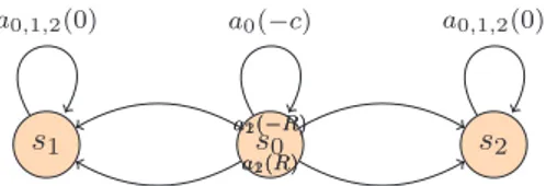
while a1 and a2 deterministically lead to absorbing states as shown in Figure 1.
Depending on the actual state s0 or s2, actions a1 and a2 give opposite rewards
(either R or −R), meaning that a1 should be chosen if actual state is s0, a2 if it
is s2. Note that R > c > 0. s0 s1 s2 s3 a1(R) a2(−R) a0 (− c) a 0 ,1 ,2 (0) a1(−R) a2(R) a0 (− c) a 0 ,1 ,2 (0)
Figure 1. Transitions of the POMDP (rewards between parenthesis)
Intuitively, there are two “good” strategies here, depending on the initial belief state:
- try to avoid the observation cost and directly choose a1 or a2;
- first observe with action a0 then act with action a1 or a2.
The observation matrix is defined as: p(o|s′) =51 0.5 0 0.5
0 0.5 1 0.5 6
We can compute the Q-values over b(s), which are the best values of each action if the optimal policy is applied next. Note that, in this simple example, the optimal policy is obvious after the first action, starting either in s0 or s2. Q-values depend on b0(s0) and b0(s2):
Qπ(b, a0) = (R − c)(b0(s0) + b0(s2)) Qπ(b, a1) = R(b0(s0) − b0(s2)) Qπ(b, a2) = R(b0(s2) − b0(s0))
Q-values over b0(s0) are shown in Figure 2-left along with the value function,
which is the best Q-value (for R = 1 and c = 0.5). We see that the optimal policy depends on the initial belief state, as expected. Also, is represented the actual value gathered by the agent according to its initial belief when the initial state of the system is s0.
1.1. Criterion Modification
Now, we add Shannon’s entropy of b(s) to the criterion at every time step, i.e. we add the expected entropy Hπ(b) denoted by : Hπ=qN
t=0H(bt). And so as, the
new criterion becomes: Jπ(b, λ) = (1 − λ)Vπ(b) + λHπ(b) The value of the belief
state entropy H(b) almost does not change when the first strategy is executed. In other hand, when the second strategy is chosen, the entropy lowers to zero at the second step. After taking action a1 or a2, the entropy value decreases, but less
than after action a0 which brings the entropy to zero. So, the mixed criterion of
the first strategy is more penalized than the one of the second strategy, because it takes into account the total value of entropies (at t = 0 and t = 1).
Qπ(b, a0) = (1 − λ)(R − c)(b0(s0) + b0(s2)) + λH(b0) Qπ(b, a1) = (1 − λ)R(b0(s0) − b0(s2)) + λ(H(b0) + H(b1)) Qπ(b, a2) = (1 − λ)R(b0(s2) − b0(s0)) + λ(H(b0) + H(b1)))
0 0.1 0.2 0.3 0.4 0.5 0.6 0.7 0.8 0.9 1 −1 −0.8 −0.6 −0.4 −0.2 0 0.2 0.4 0.6 0.8 1 b 0 (s0 ) Q π(b,a i ) a 2 a 0 a 1 0 0.1 0.2 0.3 0.4 0.5 0.6 0.7 0.8 0.9 1 −2 −1.5 −1 −0.5 0 0.5 1 b 0 (s0 ) Q π(b,a i ) a2 a 0 a 1 a0 a 2 λH(b 0 ) λH(b0 )+ λH(b1 )
Figure 2. Left: Q-values (in blue), value function (in red), also actual value gathered by the agent (in green) when system’s initial state is s0, all over b0(s0). Right: Q-values for b0(s0) = 0.2
before (blue) and after (green) criterion modification.
In order to illustrate the change in the criterion, we have computed the α-vectors for a given belief state. In the Figure 2-right the Q-values for the classical criterion and the Q-values for the modified criterion are presented for a b0(s0) =
0.2. It can be verified that the addition of the weighted entropy changes the gradient of the α-vectors. The new criterion penalizes much more the first strategy than the second one. In other words, when the weighted entropy is taken into account for this belief, the new criterion reflects in the Q-value for this belief the uncertainty, and brings on the α-vector for a0 as dominant.
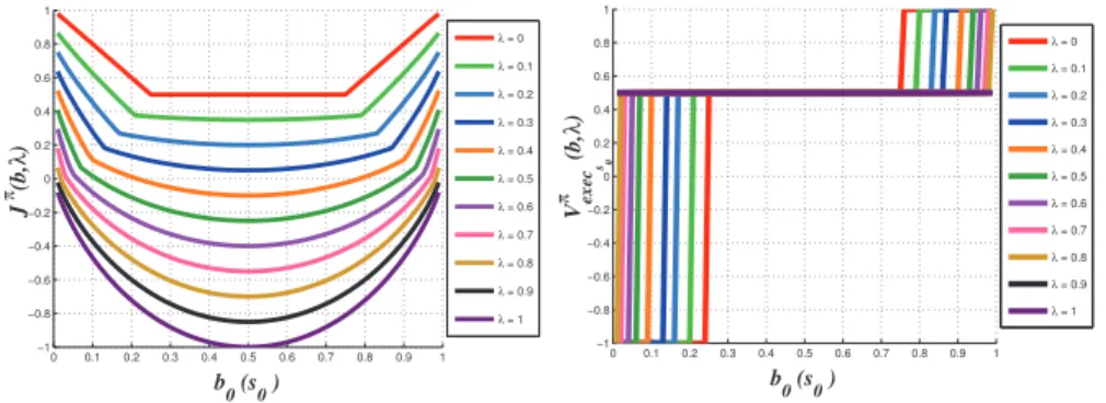
To show the change in the criterion and as a consequence, the change in the shape of the value function, we have computed the best mixed criterion in function of b0(s0) for different values of λ. Figure 3-left shows that the mixed
criterion’s shape changes a lot while varying the value of λ from zero to one: the higher the λ value is, the more the first strategy gets penalized. It also shows that the criterion is no longer linear.
Some assumptions can be overcome with this change. Figure 3-right presents the actual rewards gathered by the agent when it acts based on b(s), without knowing it is actually in state s0 at the beginning. Note the differences with
0 0.1 0.2 0.3 0.4 0.5 0.6 0.7 0.8 0.9 1 −1 −0.8 −0.6 −0.4 −0.2 0 0.2 0.4 0.6 0.8 1 b 0 (s0 ) J π(b, λ ) λ = 0 λ = 0.1 λ = 0.2 λ = 0.3 λ = 0.4 λ = 0.5 λ = 0.6 λ = 0.7 λ = 0.8 λ = 0.9 λ = 1 0 0.1 0.2 0.3 0.4 0.5 0.6 0.7 0.8 0.9 1 −1 −0.8 −0.6 −0.4 −0.2 0 0.2 0.4 0.6 0.8 1 b 0 (s0 ) V π exec s0 (b, λ ) λ = 0 λ = 0.1 λ = 0.2 λ = 0.3 λ = 0.4 λ = 0.5 λ = 0.6 λ = 0.7 λ = 0.8 λ = 0.9 λ = 1
Figure 3. Left: best mixed-criterion based on the agent’s initial belief for different λ values (λ increases from top curves to bottom ones); Right: rewards gathered at execution for different λ values depending on the agent’s initial belief when the initial state of the system is s0– which
s0 s2 s1 a1(−R) a2(R) a0(−c) a1(R) a2(−R) a0,1,2(0) a0,1,2(0)
Figure 4. Counter example of entropy addition in criterion.
the average rewards which the agent believes to gather on Figure 2-left. The closer λ is to one, the more the agent prefers observing first, so that it is less penalized if its initial belief is wrong (0.5 instead of -1). But the rewards gathered if it is right decrease also (0.5 instead of 1). So, we would like to establish some degree of confidence over b(s0) and then figure out the appropriate λ for the
problem. For this simple example, we can calculate a function λ = f(bs0), with
bs0= b0(s0), using the point where Qπ(b, a0) = Qπ(b, a2) and taking advantage
that H(b1) = H(b0) when action a2 is done.
λ(bs0) = 2Rbs0− c
2Rbs0− c + bs0ln(bs0) + (1 − bs0)) ln(1 − bs0))
This kind of modification of criterion is necessary when the agent’s initial belief (or prior) b0(s) does not correspond to real frequencies of the initial states. In
real situations, this kind of mistake often happens: the b0(s) used for the policy
calculation may not be the best approximation of the reality.
A counter example is detailed in Figure 4. We see that there is no gain in adding the belief state entropy value at every time-step, because there is no ambiguity in the initial state this case. The value function only depends on the arrival state and it will be equally penalized by the belief state entropy for each action.
Qπ(b, a0) = R|b0(s1) − b0(s2)| − cb0(s0) Qπ(b, a1) = Qπ(b0, a2) = R|b0(s1) − b0(s2)|
In the following, a mixed non-linear criterion for POMDPs is presented and the modification we made to the state-of-the-art algorithm Symbolic-PERSEUS [9] to optimize it. The next sections present some results obtained by modeling and solving a simple realistic problem which confirms the intuitions raised in this example.
2. Hybrid Optimization Criterion for POMDPs
The criterion proposed in this section models the expected cumulative discounted reward, attributed to the chosen actions, added to the expected cumulative dis-counted entropy of the belief (computed over the successive stochastic belief states), both in infinite-horizon. This two values are themselves weighted by a constant λ:
Jπ(b) = (1 − λ)Vπ(b) + λHπ(b), with (5) Vπ(b) = Eπ C∞ Ø t=0 γtr(bt, π(bt)) | b0= b D Hπ(b) = Eπ C∞ Ø t=0 γtH(bt) | b0= b D
Theorem : Bellman’s equation of the additive criterion. The optimal value func-tion of the additive criterion is the limit of the vector sequence defined by:
Jn+1(b) = max a∈A I (1 − λ)r(b, a) + λH(b) + γØ o∈Ω p(o|b, a)Jn(boa(s ′ )) J (6)
Proof. The equation 5 can be rewritten as:
Jπ(b) = Eπ C∞ Ø t=0 γt(βr(bt, π(bt)) + ρH(bt)) | b0= b D (7)
This shows that this criterion corresponds to the classic γ-discounted criterion which is the current reward added to the current entropy of the belief. It is therefore a maximization problem over γ-discounted artificial rewards equals to the real rewards plus the actual belief’s entropy.
This new Bellman’s equation permits via dynamic-programming the compu-tation of a policy that weights the immediate reward by the immediate entropy of the belief.
Heuristic. Symbolic-PERSEUS uses a heuristic function to determine the set
of reachable belief states. It initializes the belief states search with Vπ degrad=
maxs,ar(s, a), calculated from a depleted model, e.g. with an admissible heuristic
whose value must be smaller than the optimal value. The definition of the new criterion therefore requires to change this heuristic as well, in order to take into account a minimal value for H in the initialization of the reachable beliefs search calculation. The heuristic is now defined by J0 shown below.
Theorem: Heuristic for the additive criterion. An admissible heuristic to the ad-ditive criterion is given by:
J0=
(1 − λ)Vπ
degrad− λ log10(n)
1 − γ (8)
Proof. The minimal value to H(b) constrained by qni=1b(si) = 1 is given by the
Lagrangian optimization: H(b)min= n1 nlog10 3 1 n 4 = − log10(n) (9)
So: Jπ≥(1 − λ)V π
degrad− λ log10(n)
1 − γ = J0 (10)
Discussion. The criterion presented in this section is no more piecewise linear,
but algorithms such as PBVI [8], PERSEUS [11] and Symbolic-PERSEUS [9], which approach the criterion by stochastic generation of local belief states, can ap-proximate this nonlinear criterion, given that every function can be apap-proximate by a piecewise linear function.
3. Robotics Example
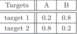
The studied model deals with an autonomous helicopter that tries to identify and track two targets. These targets are of different types, A or B. Objective of the helicopter is to land onto the target of type A, without initially knowing types of targets . This scenario combines both mission and perception objectives. Thus, this is relevant for this work because the reward optimization (implicitly) implies reducing the belief’s entropy: actually, it is necessary to reduce uncertainty over the nature of targets in order to achieve the mission. Initially, the autonomous helicopter has an a priori knowledge about the targets. It needs to track and identify each target by its actions in order to accomplish its goal. In the simula-tions studied in this work, the agent was given an initial belief state weighted and not uniforme over all possible combinations of targets types. The initial belief’s values with respect to the targets types are shown in table 1.
Table 1. Initial belief about the targets.
Targets A B
target 1 0.2 0.8 target 2 0.8 0.2
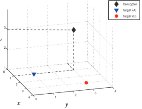
The motion space of the helicopter is modeled by a 3 × 3 × 3 grid, and the one of the targets by a 3×3×1 grid: the targets moves only on the ground (see Figure 5). The helicopter can do 7 actions: forward in x, y and z (go up), backward in
x, y and z (go down), and land. It cannot realizes more than one action at any time-step. Motions of helicopter can fail with a 10% probability, except the land action which always succeeds. Target positions are completely observable to the helicopter agent. Nevertheless, the targets change position in x and/or y, 1 time for 20 helicopter motions, but the latter cannot predict the evolution. Helicopter is allowed to land only if it is directly above a target (z = 2, as ground is z = 1). Once the helicopter has landed on the target (A) or (B), neither the helicopter nor the targets can move, and helicopter is not allowed to take-off. The observation model of the type of the targets depends on the euclidean distance from helicopter to targets as show below.
p(o′ = A | s′ = A) =1 2 1 e−d D + 1 2 and p(o′ = A | s′ = B) =1 2 1 1 − e−d D 2
0 1 2 3 4 0 1 2 3 4 1 2 3 y x z helicopter target (A) target (B)
Figure 5. Initial position of helicopter, target 1 (A) and target 2 (B).
where d is the euclidean distance between helicopter and target, and D a factor of adjustment of the exponential. This observation function allows to model the gain of information when the helicopter comes near to the target : the closer the helicopter is from the observed target, the higher the probability to observe the actual nature of the target is. The helicopter completely observes others state variables, as the positions of targets. Note that, this model does not aim at testing the effectiveness of an algorithm in terms of time of calculation nor memory used, but it is meant to illustrate different optimization criteria for the same problem.
3.1. Experimental Protocol
The optimization criterion for the POMDP is a function of the agent’s belief state, so it is optimized in terms of agent’s pessimistic and subjective belief, which have not access to the actual state of world.
On the other hand, the criterion proposed is based on rewards which really are accumulated at policy execution, weighting only the uncertainty over effects of actions. Thus we want to measure the criterion optimality from an external viewpoint i.e. from an observer outside the system, who knows perfectly the state of environment at any moment. In this paper, this omniscient observer based on a policy simulator.
For each optimized policy, we have performed 500 simulations for a 50 horizon time, i.e. for 50 successive actions executed. For γ = 0.9, this horizon is consid-ered large enough to obtain a good approximation of the criterion for an infinite horizon. The objective value function, which depends only on the current state of the environment is compute by means of Eq. (11).
Vπ(st) = 1 500 Ø 500 simulations C t Ø k=0 γkrπ(sk) | st D (11)
In this paper the optimized policies with different optimized criteria are com-pared on the basis of the same objective value, which, whatever the optimization criterion is, will always be the rewards actually collected by the agent at policy execution. To study convergence speed of the entropy of the agent’s belief, the the
current entropy of the belief entropy was calculated (statistically averaged over the runs), as shown in Eq. (12).
Hπ(bt) = 1 500 Ø 500 simulations C t Ø k=0 γkHπ(bk) | bt D (12)
Note that this measure is subjective, specific to the agent, unlike the previous measure which is objective and specific to the simulator.
3.2. Simulation and Results
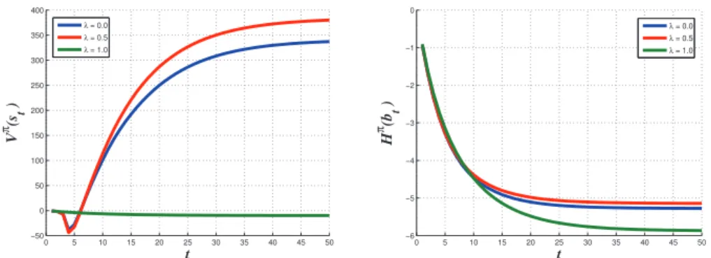
Policies have been computed for different λ values : 0, 0.5 and 1. The first value is the γ-weighted classic criterion. Note that this criterion tries to optimize only the expected cumulative discounted reward assigned to the actions and task comple-tion. The second λ value seeks to give the same importance to the accomplishment of the mission and information acquisition. And the third one optimizes only the information gain, i.e. the reduction of the entropy of the belief.
On Figure 6-left, the average of the value functions Vπ(s
t), Eq. (11), for the
3 values of λ are presented. In the first case (λ = 0), the value function Vπ(s t)
starts with negatives value; this is because the landing actions on the correct target (achieved after more than 10 simulation steps) weight less than those on the wrong one (done after 3 or 4 steps simulation) in the calculation of Vπ(s
t) due to
γ-weighting. The authors think that the landing actions on the wrong target are probably due to the small size of the grid preventing the autonomous helicopter to acquire more information before the landing happens. The helicopter, which starts with a belief state weighted towards the type of the targets, leads to land as fast as possible over a target of type (B) after only 4 or 5 steps because, at this point, it still believes that this one can be a correct target of type (A). On the other side, in simulations in which the autonomous helicopter has acquired more information from its environment, the autonomous helicopter has inverted its belief state (not presented in this section due to space) and lands on the correct target of type (A). Hence the observed reversal of the value function, which shows that the agent reacts well even to the worst case.
For the second λ value, the criterion value starts also with negative values, corresponding to the same reasons raised above. The main difference reposes on the total value gathered when t → 50. The value for the λ = 0.5 is more important than the value for λ = 0. Here the landing actions are made earlier than with the classical criterion, and so they weight more in the calculation of the Vπ(s
t)
because of the γ-weighting. The paper contribution is here illustrated, since the agent now explicitly tries to acquire more information from its environment, al-lowing it to reverse earlier its belief and finally to land more frequently (402 times
versus 390) on the correct target of type (A). A problem with the classical
cri-terion is actually its linearity in b(s): it considers that a belief state with 60% of chance of giving a reward actually brings 60% of this reward in. The non-linearity of this new criterion allows to better evaluate the value of b(s), giving less weight to smaller uncertainties. Thus we conclude that taking into account actual belief state entropy at every time-step in policy computation forces the autonomous
0 5 10 15 20 25 30 35 40 45 50 −50 0 50 100 150 200 250 300 350 400 t V π (s t ) λ = 0.0 λ = 0.5 λ = 1.0 0 5 10 15 20 25 30 35 40 45 50 −6 −5 −4 −3 −2 −1 0 t H π (b t ) λ = 0.0 λ = 0.5 λ = 1.0
Figure 6. Averaged value function of current state Vπ(s
t) (left); And cumulated weighted en-tropy of belief state Hπ(b
t) (right).
agent to better sense its environment and then, carry out its mission and receive more rewards at policy execution, which is the overall objective for the designers of an autonomous system.
With the third value of λ , the criterion optimizes only the information gain. The Figure 6-left shows that the average of Vπ(s
t) remains close to zero: the
helicopter does not try to land, it only gathers information. This is because the reward related with the task completion (landing on the target of type (A)) is no longer taken into account.
The Figure 6-right shows comparison of the subjective criterion Hπ(b t), Eq.
(12), for the 3 values of λ. Note that in the second case, average of the sum of entropy is bigger than with the classical criterion. Actually, the helicopter needs to observe its environment before task completion, which makes him reduce un-certainty over its belief state faster. This Figure also shows that the optimiza-tion of Jπ(b) allows to reduce the uncertainty faster than optimizing only Hπ(b),
because it is implicitly necessary to reduce uncertainty in order to land on the correct target. Furthermore, this work shows that the Hπ(b) optimization does
not necessarily optimizes its rate of growth at strategy execution. The mission ob-jective, integrated to the additive criterion, gives a faster lowering of uncertainty by optimizing only Hπ(b).
To conclude, the additive criterion is as good as the purely entropic crite-rion in terms of information gathering, and it converges to a bigger value than the two others criteria (purely entropic or classic γ-weighted). This is due to a second fundamental fact: the additive criterion, by forcing the optimized policy to choose actions to gain rewards over actions to gain information from time to time, actually accumulates more rewards than running the classical criterion.
4. Conclusions and Future Works
In this paper have been presented a new mixed optimization criterion for POMDPs, which aggregate the cumulative information gain (perception) and the cumulative rewards gain (mission), weighted and averaged over an infinite hori-zon. Optimality of Bellman’s equation has been underlined and proved for this
new criterion. Furthermore new admissible heuristic have been proposed for this criterion in order to use with algorithms such as Symbolic-PERSEUS.
We have experimentally demonstrated that this criterion allows the au-tonomous agent to gather information about this environment and to estimate faster its real state, compared to classic criteria (which take into account only either information gain, or rewards). Furthermore, for the additive criterion, the agent accumulates more rewards at policy execution than when it executes a pol-icy obtained with a classical criterion (which does not explicitly take into account the information gain). In some way, explicit consideration of the entropy of the belief state in addition to rewards makes the autonomous agent acquire more in-formation in order to weight his subjective view of the rewards, that it believes receiving, but may not due to its imperfect knowledge of the environment.
In the future, the influence of the λ coefficient in the additive criterion will be studied in more details. The authors believe that there is an optimal λ coefficient depending on the problem model, allowing to maximize the objective rewards actually accumulated at policy execution. The authors may also propose an opti-mization algorithm that optimizes policy and λ coefficient at the same time with respect to the modeled problem.
References
[1] W. Burgard, Dieter Fox, and Sebastian Thrun. Active mobile robot localization. In
Proceedings of IJCAI-97. Morgan Kaufmann, 1997.
[2] A.R. Cassandra, L.P. Kaelbling, and J.A. Kurien. Acting under uncertainty: Discrete Bayesian models for mobile-robot navigation. In In Proceedings of IEEE/RSJ, 1996. [3] F. Deinzer, J. Denzler, and H. Niemann. Viewpoint selection-planning optimal sequences
of views for object recognition. Lecture notes in computer science, pages 65–73, 2003. [4] R. Eidenberger, T. Grundmann, W. Feiten, and RD Zoellner. Fast parametric viewpoint
estimation for active object detection. In Proceeding of the IEEE International Conference
on Multisensor of Fusion and Integration for Intelligent Systems (MFI 2008), Seoul, Korea, 2008.
[5] L.P. Kaelbling, M.L. Littman, and A.R. Cassandra. Planning and acting in partially observable stochastic domains. Artificial Intelligence, 101(1-2):99–134, 1998.
[6] L. Mihaylova, T. Lefebvre, H. Bruyninckx, K. Gadeyne, and J. De Schutter. Active sensing for robotics – a survey. In 5th Intl Conf. On Numerical Methods and Applications, pages 316–324, 2002.
[7] Lucas Paletta and Axel Pinz. Active object recognition by view integration and reinforce-ment learning. Robotics and Autonomous Systems, 31:71–86, 2000.
[8] J. Pineau, G. Gordon, and S. Thrun. Point-based value iteration: An anytime algorithm for POMDPs. In Proc. of IJCAI, 2003.
[9] P. Poupart. Exploiting structure to efficiently solve large scale partially observable Markov
decision processes. PhD thesis, University of Toronto, 2005.
[10] M.T.J. Spaan and P.U. Lima. A decision-theoretic approach to dynamic sensor selection in camera networks. In Int. Conf. on Automated Planning and Scheduling, pages 279–304, 2009.
[11] M.T.J. Spaan and N. Vlassis. A point-based POMDP algorithm for robot planning. In
IEEE International Conference on Robotics and Automation, volume 3, pages 2399–2404.
IEEE; 1999, 2004.
[12] M.T.J. Spaan and N. Vlassis. Perseus: Randomized point-based value iteration for POMDPs. JAIR, 24:195–220, 2005.
[13] M. Sridharan, J. Wyatt, and R. Dearden. HiPPo: Hierarchical POMDPs for Planning Information Processing and Sensing Actions on a Robot. In Proc. of ICAPS, 2008.