This is an author-deposited version published in:
http://oatao.univ-toulouse.fr/
Eprints ID: 3229
To cite this document:
MORLIER, Joseph. A pedagogical image processing tool to
understand structural dynamics. In: MAC XXVIII A Conference and Exposition on
Structural Dynamics Structural Dynamics and Renewable Energy, 01–04 Feb 2010,
Jacksonville, USA.
Any correspondence concerning this service should be sent to the repository
administrator:
staff-oatao@inp-toulouse.fr
A pedagogical image processing tool to understand structural dynamics
Joseph Morlier
Université de Toulouse, ISAE DMSM, Campus SUPAERO,10 av. Edouard Belin
BP54032 - 31055 Toulouse Cedex 4 – France
joseph.morlier@isae.fr
Abstract
This paper presents a framework and one pedagogical application of motion tracking algorithms applied to structural dynamics. The aim of this work is to show the ability of high speed camera to study the dynamic characteristics of simple mechanical systems using a marker less and simultaneous Single Input Multiple Output (SIMO) broadband analysis. KLT (Kanade-Lucas-Tomasi) trackers are used as virtual sensors on mechanical systems video. First we introduce the paradigm of virtual sensors in the field of modal analysis using video processing. Then we present a pedagogical example of flexible beam (Fishing rod) video. From KLT tracking we extracted displacements data (virtual sensors) which are then enhanced using filtering and smoothing and then we can identify natural frequency and damping ratio from classical modal analysis. The experimental results (mode shapes) are compared to an analytical flexible beam model showing high correlation but also showing the limitation of linear analysis. The main interest of this paper is that displacements are simply measured using only video at FPS (Frame Per Second) that respects the Nyquist frequency. There is no target needed on the structure only few critical pixels that are good features to track and which become virtual sensors.
1. Introduction
In order to achieve the right combination of material properties and service performance the dynamic behavior is one of the main points to be considered. To better understand the dynamic behavior of the structure we need to characterize the resonances of the structure. A common way of doing this is to define its modal parameters i.e. natural frequency, damping ratio and mode shape [1]. The goal of our work is to develop a method to replace classical contact accelerometers based instrumentation with an optical camera working with an intelligent software in order to continuously assess the dynamic parameters of the structure. Previous works [2-5] obtained modal parameters by introducing real targets on the structure or by studying simple structure in ideal conditions. Real time displacement measurement have been done using different approach of digital image processing techniques (texture recognition algorithm) on a flexible bridge [6] or using LED targets (colour filtering) [7]. In our previous work [8] displacement of a bridge under harmonic excitation was reconstructed by using video openCV framework. Such bridges have low natural frequencies within 5 Hz and maximum displacement of several centimetres. In a previous paper [9] we continue in studying the linear dynamic response of a helicopter blade using a broadband excitation. Here the size of the structure is smaller: so the frequencies increase and the experimental setup changes (need of high speed camera to verify the Nyquist criteria) and the high displacement of the fishing rod permit to study more modes.
This method can be used in structural dynamics according to three important hypothesis; firstly the number of Frame Per Second (FPS) verifies the Nyquist frequency criteria, secondly the camera axis is perpendicular to the studied 2D structure (to avoid angular errors) and finally the global displacement (in pixels) must be superior to the pixel resolution if not the mode would not appear in the Frequency Response Function (FRF). According to these hypotheses the main drawback of our works is that industrial applications are limited to large structures because they have lower frequencies and larger displacements. But however it remains interesting for educational purposes; it offers a simple measurement tool to understand and visualize structural dynamics engineering problems. From the application point of view, video camera and motion tracking algorithm replaces accelerometers for bending displacement measurements under broadband excitation. One advantage of this non contact measurement method (versus Laser Doppler Vibrometer) is that we can measure in one test several simultaneous outputs for SIMO modal analysis.
A way to detect moving objects is by investigating the optical flow which is an approximation of two dimensional flow field from the image intensities. It is computed by extracting a dense velocity field from an image sequence.
The optical flow field in the image is calculated on basis of the two assumptions that the intensity of any object point is constant over time and that nearby points in the image plane move in a similar way [10]. Additionally, the easiest method of finding image displacements with optical flow is the feature-based optical flow approach that finds features (for example, image edges, corners, and other structures well localized in two dimensions) and tracks their displacements from frame to frame. The LK [11] tracker is based upon the principle of optical flow and motion fields [12-14] that allows to recover motion without assuming a model of motion. For practical purposes we use this algorithm on the flexible beam example in order to track the motion of the target pixels and reconstruct displacement signals. It offers various advantages like stable and accurate motion results in non optimal environment. The paper is arranged in three parts, the first introduces the theoretical background of motion tracking and discusses of the optical flow algorithm in the domain of vibration measurement. Then we present the experiment of vibrating fishing rod. Finally the structural characterisation of a flexible beam is studied using virtual sensors data processing. The dynamic parameters are extracted from FRF reconstruction and experimental results are compared with analytical solutions.
2. KLT motion tracking
Kanade-Lucas-Tomasi (KLT) features may be used to describe general motions within video images. The KLT algorithm finds several thousand features in each frame of video. It then attempts to find a correspondence between the features in one frame with the features in the next. The origins of the Kanade-Lucas-Tomasi Tracker go back to the work of Lucas and Kanade [11]. They introduced a way to select features that is explicitly based on the tracking equation. Their intention is to select those features that make the tracker work best. They also proposed using an affine model of image motion to monitor feature dissimilarity between the first and the current frame. Most of the time, it is impossible to determine the location of a single pixel in the subsequent frame based only on local information. Due to this, small windows of pixels are used as features. The goal of tracking is to determine the displacement d of a feature window from one frame to the next (Figure 1).
I(x,y)
J(x,y)
Figure 1: Optical flow principle. Pixel motion from image I to image J is estimated solving the pixel correspondence problem: given a pixel in I, look for nearby pixels of the same color in J. Two key assumptions are needed: color constancy (a point in I looks the same in J) and small motion (points do not move very far).
The displacement is chosen as to minimize the dissimilarity between two feature windows, one in image I and one in image J:
∫∫
+
=
W 2w(x)dx
I(x)]
-d)
[J(x
ε
(1)where W is the given feature window, x = [x, y]T are coordinates in the image and d = [dx, dy]T is the displacement. The weighting function w(x) is usually set to the constant 1. The aim is to find the displacement d that minimizes the dissimilarity. For this, we differentiate Equation (1) with respect to d and equate it to zero.
∫∫
=
∂
+
∂
+
=
∂
∂
W0
w(x)dx
d
d)
J(x
I(x)]
-d)
[J(x
2
d
ε
(2)Using the Taylor series expansion of J about x, truncated to the linear term, we obtain:
J(x)
y
d
J(x)
x
d
J(x)
d)
J(x
x y∂
∂
+
∂
∂
+
≈
+
Putting this into Equation (2) yields
∫∫
+
=
=
∂
∂
W T0
g(x)w(x)dx
d]
g(x)
I(x)
-[J(x)
2
d
ε
Where
∂
∂
∂
∂
=
J
y
J
x
g(x)
Rearranging terms yields a linear 2 × 2 system:
Zd = e (3)
Where Z is the 2 × 2 matrix:
=
∫∫
W T
w(x)dx
(x)g(x)
g
Z
and e is=
∫∫
W(x)dx
J(x)]g(x)w
-[I(x)
e
Equation (3) is only approximately satisfied, because of the linearization of Equation (2). However, the correct displacement can be found by minimizing Equation (3) using a Newton-Raphson algorithm.
Several interest operators have been proposed based on intuitive ideas of what good features should look like. Shi and Tomasi [15] propose a more principled criterion that is optimal by construction: “A good feature is one that can be tracked well”. Thus our virtual sensors should be located on good feature for correct displacement measurements.
When dealing with dynamic systems, it is clear that the temporal sampling frequency (or frame rate) fs must be greater than 2Bt (Equation 4), in order to avoid aliasing in the temporal direction (Nyquist criteria). If global motion is assumed with constant velocities vx and vy (in pixels per standard-speed frame) and spatially band limited image with Bx and By as the horizontal and vertical spatial bandwidths (in cycles per pixel), then the minimum temporal sampling frequency fs (in cycles per speed frame) to avoid motion aliasing is given by
vy
2By
vx
2Bx
2Bt
fs
=
=
×
+
×
. (4)The assumptions of optical ideal conditions and ideal blur filter have been done here. Typical high speed camera uses a state-of-the-art CMOS sensor that records images at 1000 FPS at 1024x768 pixel resolution (or more).
3. Experiment : Vibrating fishing rod
In this experiment a pixel represents 2.12 mm using a video at a resolution of 1024x256pixels
(
sf
=
0
.
1
m 47
/
Pixels
), so only the first three bending modes (higher displacements than 2.12 mm) can bemeasured. After 30 Hz the others modes (displacements inferior to the resolution) induce only noise. Figure 2 presents the cantilever flexible beam experiment. The LK optical flow is used to follow 9 targets (green arrows) in bending along Y displacement. These targets become virtual displacement sensors which allow doing a SIMO analysis in only one test. The main experimental hypothesis is to constrain the flexible beam in Y direction (using blocks). The dynamic behaviour of the fishing rod is more complex (chaotic) as the beam has a tapered geometry, the material is composite and the behaviour remains nonlinear due to large deflections and/or rotations.
Figure 2: Cantilever flexible beam example: KLT trackers are used to follow 9 targets in bending (Y displacement). The targets are numbered from 1 to 9.
The main problem occurs in signal reconstruction (displacement). In fact target pixels (which move around x axis) create partial modal data, so displacement signals are irregular data. Thus the small linear displacement hypothesis is used (stability diagram of the Figure 3) to enhance the resolution of the motion and to compensate the missing data,. If the absolute value of x (relative displacement on abscissa) is less than 3 pixels the data is used, otherwise it is not implemented.
0 500 1000 1500 2000 2500 3000 3500 -0.5 0 0.5 1 1.5 2 2.5 Images X d is p la c e m e n t
Figure 3: Using this stability diagram the linearity hypothesis is checked: Each target has does not vary in X direction.
1
X
Y
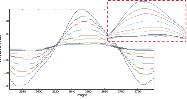
Some pre-processing like windowing (Hanning) and filtering (low pass) have been done. The transfer functions have been estimated using tfestimate in Matlab. Figure 4 illustrates the effect of a running moving average (size of the window is 5) on the temporal signals. All these signal processing tools aim at obtaining smoother FRFs for more precise analysis.
2580 2600 2620 2640 2660 2680 2700 2720 -0.06 -0.04 -0.02 0 0.02 0.04 Images Y d is p la c e m e n t (m )
Figure 4: Effect of the moving average function on the temporal signal. This pre-processing aims at obtaining smooth FRFs.
The type of excitation (pulling down) offers a correct bandwidth at low frequency which allows the identification of the first three modes. The excitation level is the static-force that creates the deflection (1.96N) which induces the free decay.
The results of the FRFs reconstruction permit to do a classical modal analysis extracting the three dynamic parameters (frequencies, damping ratios and mode shapes). These parameters which characterize the dynamic behavior of the beam are estimated from FRFs using classical SDOF frequency method called Rational Fraction Polynomial (RFP, [18]) around resonances
f
i±
1
Hz
. Results are listed in Table 1 and can be compared with very good correlation to previous results from classical accelerometers sensors.) f ( E
σ
(
f
)
E(ξ)σ
(
ξ
)
3.32 (Hz)
6E-4
0.93 (%)
3E-4
9.78 (Hz)
8E-2
0.96 (%)
3E-3
21.69 (Hz)
3E-2
0.73 (%)
3E-3
Table 1: Estimated mean E and standard deviation
σ
for frequencies f and damping ratios ξ for three first modes extractedusing RFP.
The figure 5 shows filtered FRFs (9 measurement points) and the result of the identification of the first resonance at 3.32 Hz for each transfer functions. Thus the FRF correlation between experimental data and identified data is very good for each virtual sensor.
5 10 15 20 25 30 35 40 45 50 -150 -100 -50 0 50 Frequency (Hz) F R F m /N ( d B ) 5 10 15 20 25 30 35 40 45 50 -150 -100 -50 0 50 Frequency (Hz) R e b u ilt F R F m /N ( d B )
Figure 5: Filtered FRFs form 9 measurement points and identification of the first resonance at 3.32 Hz using SDOF RFP method.
4. Data Analysis: Fitting theoretical mode shapes
In order to validate our experiment results our first approach was to use the theory of the tapered beam [19]. The aim was to compare experimental frequency ratio with theoretical to identify the pseudo frequencies
β
i of the beam. According to the results of table 2, a good correlation of experimental data is found with the tapered beam theory. Taking into account that for uniform and tapered beam the second frequency has almost the same value, it is easy to deduce from these ratios the estimation ofβ
i:β
1=
1
.
05
,
β
2=
1
.
81
,
β
3=
1
.
60
(Table 2).Frequency
ratio Tapered theory Experimental Error
2 1 2 1 2
=
β
β
ω
ω
2.61 2.945 12% 2 2 3 2 3
=
β
β
ω
ω
1.81 2.21 22%Table 2: Estimated frequency ratios (tapered theory) compared with experimental results.
We can also notice that higher error occurs for the third parameter identification due to the nonlinear behaviour of this mode.
The mode shape describes the structure’s motion when it is vibrating at a particular frequency. Classically, the equation used to represent a uniform (regular section) beam under free vibration can be written as follows:
0
)
,
(
)
,
(
4 4 2 2=
∂
∂
+
∂
∂
t
x
v
x
EI
t
x
v
t
S
ρ
where x is the longitudinal coordinate, v is the transversal displacement of the beam in Y direction (which is perpendicular to X), t is time, E is the Young’s modulus, S is the cross section area, I is the planar moment of inertia of the cross section, L is the length and
ρ
is the density of the beam. Assuming that bending stiffness isindependent of time and that the steady state vibration has a harmonic form, we get:
0
)
x
(
Y
dx
)
x
(
Y
d
4 4 4=
−
λ
Using separated variables and solving the differential equation, we can express the mode shape as:
)
x
sin(
A
)
x
cos(
A
)
x
sinh(
A
)
x
cosh(
A
)
x
(
Y
i=
1iλ
i+
2iλ
i+
3iλ
i+
4iλ
i (5)Where the spatial frequency of the ith mode is defined as
EI
m
i iω
λ
2=
withi
=
1
...
n
.Using Equation 5 experimental data can be fitted with the analytical equation of the dynamic motion of a beam using least square method with very good correlation (
R
2f
0.98
) for the first two modes (figure 9). All the mode shapes highlight local singularities due to local change in the beam materials properties (beam having 15 variable sections). It can be noticed that the coefficient estimated from the analytical fit are typical of the Fixed-Free bending mode behaviour (opposite coefficientsA
1i/A
3iandA
2i/A
4i [20]) which correlate well the shape of the mode (Figures 6). 0 0.5 1 1.5 2 2.5 0 0.1 0.2 0.3 0.4 0.5 0.6 0.7 0.8 0.9 1 Beam length (m) N o rm a lis e d M o d e s h a p e ( M o d e 1 ) 0 0.5 1 1.5 2 2.5 0 0.2 0.4 0.6 0.8 1 Beam length (m) N o rm a liz e d M o d e s h a p e ( M o d e 2 )Figure 6 : First mode shape extracted using experimental data: The global content of this mode is close to the first mode of an uniform beam. Some important singularities appear at the discontinuities of the fishing rod. For the second mode, the experimental data correlate well with the general model of mode shape. This mode is very close from second mode shape of Fixed-Free beam, expected for several zones that highlight the discontinuities of the fishing rod.
General model: f(x) =
a.cos(b.x)+c.sin(b.x)+d.cosh(b.x)+e.sinh(b.x) Coefficients R² RMSE
Mode 1 a = -0.232 b = 1.225 c = 0.116 d = 0.231 e = -0.180 0.992 0.040 Mode 2 a =-0.093 b =1.8 c =-0.099 d = 0.071 e =0.067 0.986 0.043
Table 3: Estimated parameters of the fit of experimental mode shapes with analytical formula (Eq 5). The R² and RMSE coefficients show very good correlation with the general model.
The motion of each part of the flexible beam has been assumed to be harmonic as explained before. The spatial part for each section is given by Eq 6 where indice i is the ith mode and j is the jth section [21]:
)
sin(
)
cos(
)
sinh(
)
cosh(
)
(
x
A
1x
A
2x
A
3x
A
4x
Y
ij=
ijλ
ij+
ijλ
ij+
ijλ
ij+
ijλ
ij (6)If the number of sections is n then the number of unknown parameters in the final solution is 4n. Matching the boundary conditions at each of the n-1 interfaces, as described in Eq. (6), insures continuity between the sections and equilibrium of the total bending moments and internal shear forces (Figure 10).
Figure 7: The boundary conditions are matched at each of the (n-1) interfaces between the elements. For each interface there are 4 equations in order to insure continuity and equilibrium for the shear force and bending moment. At the two extremities, the conditions are the usual ones for a beam with a clamped and a free end.
The poor global third mode shape regression can be explained by the fact that Eq 5 is used instead of Eq 6. Then the main influence is the beam geometry (the fishing rod has 15 section) which should be fitted using a piecewise multiple fit tool to adjust the experimental data with enhance model of stepped beam (Eq 6). In addition normalization of this mode shape (Figure 8) increases the nonlinear behaviour (the real amplitude is very small compared to the first mode).
0 0.5 1 1.5 2 2.5 3 0 0.1 0.2 0.3 0.4 0.5 0.6 0.7 0.8 0.9 1 Beam length (m) N o rm a liz e d M o d e s h a p e ( M o d e 3 )
Figure 8 : Third mode shape extracted using experimental data highlights a complex behaviour: the 15 zones of the stepped beam are describes by red dotted stem. Each part of the beam should be identified with a different parameter (Eq 6).
In the experimental results the spatial sampling is not regular (good features to track are zones that have good contrast i.e. stepped zones of the fishing rod), so the spatial resolution is very poor but easy to interpolate. One of other limitations is that the influence of the camera viewpoint and calibration has not being taken into account in this study. The other disadvantage is that in some applications the small linear displacement hypothesis is not verified. It induces some instabilities of the targets which lead to several partial displacement measurements instead of one fixed (x direction) virtual sensor displacement (in bending; y displacement). Finally the vertical sensitivity will be low due to the size of the deflection compared to the length of the beam. It allows us to identify with only the two first modes with accuracy; the others have complex behavior or displacement inferior or close to the pixel, so that the noise influences more on the mode shape estimation process. Nevertheless the main interest of this method is that no targets need to be placed on the structure and also no time consuming computation is needed (for real time applications) even if several virtual sensors are to be tracked.
Conclusion
The main goal of this paper is to show a pedagogical image processing tool to understand structural dynamics. OpenCV framework can easily be used for displacemet measurement on a video of a vibrating system according the speed of camera respect the Nyquist criteria. KLT trackers are simply used as virtual sensors to measure displacement on video choosing good features to track on the image. We succeed to estimate the first three main modes of a flexible beam (cantilever composites fishing rod) under broad band excitation. For educational purposes, this simple application can also be used with the help of less expensive tools than high speed camera, e.g. with a classical camera (frequency max is 12.5Hz at image resolution of 1024*768 pixels). Finally it will be interesting to develop a 3D framework with several synchronised camera to continuously monitor an important structure like a bridge.
Acknowledgments
The author want to thanks Guilhem Michon for his technical help and the 2nd year students Paul Sebellin and Emmanuel Godard of ISAE campus-Supaero for being part of this pedagogical research project.
References
[1] D. J. Ewins, Model Testing: Theory and Practice, Research Studies Press, 1984.
[2] P. Olaszek, Investigation of the dynamic characteristic of bridge structures using a computer vision method. Measurement 25 (1999) 227–36.
[3] S. Patsias and W.J. Staszewski, Damage detection using optical measurements and wavelets, Vol 1, Structural Health Monitoring, 1 (2002) 5–22.
[4] U.P. Poudel, G. Fu and J. Ye, Structural damage detection using digital video imaging technique and wavelet transformation, Journal of Sound and Vibration 286 (2005) 869–895.
[5] J.J. Lee, M. Shinozuka, A vision-based system for remote sensing of bridge displacement, NDT and E International 39 (5) (2006) 425-431.
[6] J.J. Lee, M. Shinozuka, Real-time displacement measurement of a flexible bridge using digital image processing techniques, Experimental Mechanics 46 (1) (2006) 105-114.
[7] A.M. Wahbeh, J.P. Caffrey, S.F. Masri, A vision-based approach for the direct measurement of displacements in vibrating systems, Smart Materials and Structures, Vol; 12 (5) (2003) 785-794.
[8] J. Morlier, P. Salom, F. Bos, New image processing tools for structural dynamic monitoring, Key Engineering Materials Vol. 347 (2007) 239-244.
[9] J. Morlier, G. Michon, Virtual vibration measurement using KLT motion tracking algorithm, Journal of Dynamic Systems, Measurement and Control (In Press 2009)
[10] J.K. Aggarwal, and N. Nandhakumar, On the computation of motion from sequences of images - A review, in: Proceedings of the IEEE, Vol. 76(8), 1988 , pp. 917-935.
[11] B.D. Lucas and T. Kanade, 1981, An iterative image registration technique with an application to stereo vision, in: Proceedings of Imaging understanding workshop, pp 121-130.
[12] J.L. Barron, D.J. Fleet, and S.S. Beauchemin, Performance of Optical Flow Techniques, International Journal of Computer Vision, 12 (1994) 43–77.
[13] S. Lim, J.G. Apostolopoulos, A.E. Gamal, Optical flow estimation using temporally oversampled video, IEEE Transactions on Image Processing14 (2005) 1074- 1087.
[14] J.Y. Bouguet, Pyramidal Implementation of the Lucas Kanade Feature Tracker, openCV documentation.
[15] J. Shi and C. Tomasi. Good features to track, In: Proceedings IEEE Computer Society Conference on Computer Vision and Pattern Recognition, 1994, pp. 593-600.
[16] Information on http://opencv.willowgarage.com/wiki/
[17] C.C. Chang, Y.F. Ji, Flexible videogrammetric technique for three-dimensional structural vibration measurement, 2007 Journal of Engineering Mechanics 133 (6), pp. 656-664.
[18] M. H. Richardson and D. L. Formenti, Parameter Estimation from Frequency Response Measurements using Rational Fraction Polynomials, in: Proceedings of the International Modal Analysis Conference,1982, pp.167-181.
[19] H. Wang and W.J. Worley, Tables of natural frequencies and nodes for transverse vibration of tapered beams, NASA CR 443, 1966.
[20] S.S. Rao, Mechanical vibrations, Prentice hall, 2003.