HAL Id: hal-03176359
https://hal.archives-ouvertes.fr/hal-03176359
Submitted on 22 Mar 2021
HAL is a multi-disciplinary open access
archive for the deposit and dissemination of
sci-entific research documents, whether they are
pub-lished or not. The documents may come from
teaching and research institutions in France or
abroad, or from public or private research centers.
L’archive ouverte pluridisciplinaire HAL, est
destinée au dépôt et à la diffusion de documents
scientifiques de niveau recherche, publiés ou non,
émanant des établissements d’enseignement et de
recherche français ou étrangers, des laboratoires
publics ou privés.
A finance driven supply chain network design model
Hamidreza Rezaei, Nathalie Bostel, Vincent Hovelaque, Olivier Péton
To cite this version:
Hamidreza Rezaei, Nathalie Bostel, Vincent Hovelaque, Olivier Péton. A finance driven supply chain
network design model. MOSIM 2020 : 13th International Conference on Modeling, Optimization and
Simulation, Nov 2020, Agadir (virtuel), Morocco. �hal-03176359�
A FINANCE DRIVEN SUPPLY CHAIN NETWORK DESIGN
MODEL
Hamidreza REZAEI1,2, Nathalie BOSTEL3,2, Vincent HOVELAQUE4, Olivier P ´ETON1,2 1IMT Atlantique, 4 rue Alfred Kastler, Nantes, France
2LS2N, UMR CNRS 6004, Nantes, France 3 Universit´e de Nantes, Nantes, France
4 Univ-Rennes, CNRS, CREM - UMR 6211, F-35000 Rennes, France
hamidreza.rezaei@imt-atlantique.fr, nathalie.bostel@univ-nantes.fr, vincent.hovelaque@univ-rennes1.fr, olivier.peton@imt-atlantique.fr
ABSTRACT: We propose a supply chain network design model focusing on the interactions between logistic and financial considerations. From the logistic point of view, this model determines the optimal location of production facilities and the assignment of these facilities to customers. From the financial point of view, it plans logistics decisions such that a financial indicator is maximized. We propose to use the Adjusted Present Value (APV) as the objective function.
KEYWORDS: Supply chain, network design, facility location, finance, Adjusted Present Value, Z-score
1 INTRODUCTION
Supply Chain Network Design (SCND) aims at opti-mizing strategic decisions such as ”where” and ”when” to locate facilities. It also determines the capacity of facilities and product flows in logistics networks. The primary goal in classical SCND models is to maximize the profit or, equivalently, to cut logistics costs. In this paper we focus on the interactions between the logistic and financial considerations in SCND. At least two financial impacts must be studied. The first one concerns the funding of logistics decisions. There are several means to finance big investment over a long term horizon. This funding may use inter-nal financial resources that the company accumulated prior to the investment. In this case, the investment decision must be anticipated. It can also be financed by borrowing. These two funding levers modify the financial structure of the company and, subsequently, some of its financial ratios. This may have a consid-erable impact on the future value of the company. The importance of incorporating financial consider-ations into strategic decisions, in particular supply chain management decisions, has been reported many times in the literature. Shapiro (2004) discusses the links between supply chain, demand, and corporate financial decisions at the strategic level. He men-tions the strong interaction between the financial fac-tors and the strategic planning of firms and organi-zations. In the context of closed-loop supply chain network design, Ramezani et al. (2014) mention that the majority of studies consider the financial aspects
as endogenous variables, and only very few studies consider these aspects as exogenous variables used in constraints and in the objective function. It is strik-ing to see that financial considerations are very often considered in the literature as side constraints, but are never in the core of the decision model. The goal of this paper is to fill this gap by proposing a mathe-matical model for the joint optimization of the supply chain network design and of the firm’s value.
2 FINDING A RELEVANT FINANCIAL OBJECTIVE FUNCTION
2.1 Capital structure optimization
The question of defining the optimal capital struc-ture (Modigliani and Miller, 1963) refers to the debt over equity ratio. This question arises when large in-vestments must be decided, which is exactly the case in strategic supply chain management decisions. The corresponding large investments can be financed by the equity and by the debt. In the first case, the necessary funds are supported by the shareholders or generated by the firm’s activities. In the second case, they are borrowed from banks and financial institu-tions. The most significant incentive of debt financ-ing, called tax shield benefit (TSB) is related to the corporate income tax system. Given that the interest expenses associated with the debt are tax-deductible, the TSB is proportional to the corporate tax rate as well as the amount borrowed to the bank. It is thus, easy to calculate.
MOSIM’20 - November 12-14, 2020 - Agadir - Morocco
The main risk of debt financing is the possibility of bankruptcy if a firm is unable to repay debts. There is a vast literature dedicated to the evalua-tion of bankruptcy cost. We consider the expected bankruptcy cost, which combines an estimation of the cost of bankruptcy, denoted BC and the probability π of going bankrupt. The expected bankruptcy cost EBC is estimated as follows (Damodaran, 2012):
EBC = π × BC.
The valuation of the bankruptcy cost BC follows the model of Leland (1994). Let U V represent the unlev-ered value of the firm, i.e. its value under all-equity financing. When bankruptcy occurs, a firm loses a fraction 0 ≤ β ≤ 1 of its unlevered value. Then,
BC = β × U V.
Myers (1984) introduced the trade-off theory, in which the TSB is balanced by the dead-weight bankruptcy cost. According to this theory, there is a debt to equity ratio, driving the firm to its maxi-mum value.
This mechanism is illustrated by Figure 1. When the debt level increases (horizontal axis), both the value of TSB and BC increase. It is assumed that the tax shield, represented by the black solid line increases roughly linearly, while BC is nonlinear. Thus, the firm’s value (represented by the blue curve) first in-creases, then reaches an optimal value and then de-creases. The highest point of the firm’s value curve helps determine the optimal debt value.
2.2 Z-score
The Z-score is an econometric scoring tool, developed in the late 60s (Altman, 1968; Beaver, 1968), used in decisions to grant credit limits. It is one of the most popular bankruptcy predictors for companies and or-ganizations. Its main use is to establish a probability of default at 2 years on the basis of 5 financial ra-tios. We use the following Z-score formula for private manufacturing companies:
z = 0.717X1+ 0.847X2+ 3.107X3+
0.420X4+ 0.998X5, (1)
where X1 is the Working capital/Total assets ratio,
X2is the Retained Earnings/Total assets ratio, X3is
the Earnings Before Interest and Taxes (EBIT)/Total assets ratio, X4is the Book value of equity/Book value
of total liabilities ratio and X5is the Sales/Total
As-sets ratio.
The primary goal of the Z-score is to predict bankruptcy. Its value can be converted to a prob-ability π of bankruptcy with a logistic function (see,
e.g. Hillegeist et al. (2014) and Kallunki and Pyykk¨o (2013)).
π = e
−z
1 + e−z. (2)
2.3 Adjusted Present Value (APV)
Let us first recall the definition of the Net present Value (NPV). It is defined as the value of a project’s future cash flows (positive or negative), translated into today’s money i.e., the difference between a project’s value and its costs over time. Given a set T of time periods, the values of the profit and fixed assets at each period t ∈ T and the cost of equity rE,
N P V = P
t∈T
P rof itt−F ixedAssett
(1+rE)t is used as an
objec-tive function in numerous SCND papers, especially in models describing real-life applications or complex supply chains.
The Adjusted Present Value (APV), proposed by My-ers (1974) is mainly used for the valuation of invest-ment projects. Practically, it is calculated as follows: AP V = N P V + T SB − EBC. (3) The main principle of the APV is to adjust the un-levered value of the firm by considering the debt ef-fect. The total enterprise value equals the sum of the values of the operating assets plus the present value of debt tax shields. The main contribution of our mathematical model is to adopt APV as the objec-tive function in a classical SCND model, instead of classical cost based objective functions, so as to max-imize the overall firm’s value.
3 PROBLEM SETTINGS AND MATHE-MATICAL FORMULATION
3.1 Problem statement
We consider a supply chain consisting of a set I of cus-tomers delivered from a set J of potential production centers belonging to the same company. Customers’ locations and demands are known and considered de-terministic over a time horizon T decomposed in dis-crete time periods, typically years. We also define T∗ = T \{0}. The main goal of the SCND problem is to select a subset of production centers among the whole set J and to assign customers’ demand to these production centers, at each time period, so as to max-imize the adjusted present value of the company. Satisfying customers’ demand requires a certain num-ber of logistic decisions: opening production facilities, setting production levels and carrying the goods from facilities to customers. The mathematical model pre-sented in this section aims at determining the list of
Firm Value
Debt Level
Optimal debt value Firm value under all-equity financing (UV)
Firm value considering both tax shield and bankruptcy cost (UV+TSB-EBC) Firm value considering only taxshield (UV+TSB) Tax shield benefit (TSB)
Expected Bankruptcy cost (EBC)
Figure 1 – Trade-off theory for the determination of the optimal debt value
candidate facilities selected, and the product flows from these facilities to customers at each time period, in order to maximize an objective function based on both financial and logistic goals. Since one of the main goals of this paper is to show the interactions between logistic and financial decisions, we adopted a set of simple logistic rules that are not too con-straining. We assume that there is no closing option for the facilities. In other words, once a facility is selected, it will stay open until the end of the time horizon. The generalization of this work to a network with both opening and closing options does not raise theoretical difficulties.
The main assumption is that it is not mandatory to serve every particular customer’s demand. This can be justified by at least two reasons. First, some cus-tomers may be simply too far from production cen-ters, so that delivering them would result in a loss of money. Second, enforcing the delivery to all cus-tomers would generate unrealistic solutions in which large fixed cost would be paid to open facilities that deliver only a few customers. We do not impose any single sourcing constraint: customers can be deliv-ered from distinct facilities at distinct periods. How-ever, no partial satisfaction of a particular customer’s demand is authorized. Moreover, if a customer’s de-mand is satisfied within a given time period, then it must be satisfied again in all subsequent time peri-ods. Unsatisfied customers’ demands are simply lost ; back-orders are not authorized. For each time pe-riod, the fraction of the total demand that is satisfied is called fill rate.
All supply chain operations have a potentially large
cost that must be financed with either debt or equity. Companies generally mix debt financing and equity financing. Thus, for a given decision, the amount to be borrowed to banks and the duration of repayment varies with respect to this mix. We define a set B of available bank offers. Each bank offer is modeled by a tuple containing the maximum amount of money that can be borrowed, an interest rate and a repayment duration.
Incorporating financial decisions into an SCND prob-lem amounts to select a subset of candidate bank offer and optimize the financial flows of the company. The objective function of the optimization problem con-sidered is to maximize the firm’s value at the end of the time horizon, where the APV described in sec-tion 2.3 is used as a proxy for the firm’s value. We consider only two modes for financing supply chain strategic decisions: equity (using the available cash accumulated in previous periods) and debt (selecting bank offers). This study does not consider capital in-crease, which decision depends on strategic objectives that can hardly be modeled by mathematical models. Moreover, our decision making framework does not consider any decision at the tactical or operational decision levels. The next sections detail the proposed MILP formulation. Section 3.2 describes the variables and constraints related to logistic decisions. Section 3.3 does the same for financial decisions. Section 3.4 describes the calculation of the APV.
MOSIM’20 - November 12-14, 2020 - Agadir - Morocco
3.2 Logistic constraints
For any j ∈ J and t ∈ T , the binary variables yjt
equal 1 if the facility j ∈ J is selected at period t ∈ T , and 0 otherwise. As mentioned before, once a facility is selected, it cannot be closed later. Besides, the number of facilities selected is bounded above by a number Jmax. These assumptions are modeled by
constraints (4) and (5).
yj,t−1≤ yjt ∀j ∈ J, t ∈ T∗ (4)
X
j∈J,t∈T∗
yjt− yj,t−1≤ Jmax (5)
Constraints (6), (7), (8) and (9) are related to the delivery of customers. Due to different trade rules between geographical areas as well as various logistic constraints, it might be practically impossible to de-liver some customers from some facilities. Thus, we introduce the binary notation vijwhich is set at value
1 if the customer i ∈ I can be delivered by the facil-ity j ∈ J . Moreover, we denote by qijt the quantity
delivered by facility j ∈ J to customer i ∈ I at time period t ∈ T .
With these notations, constraints (6) set qijt to 0 if
customer i ∈ I cannot be served by facility j ∈ J or if facility j ∈ J is not operating at period t. The binary variables θit take value 1 if customer i ∈ I is
served at period t ∈ T , and 0 otherwise. Constraints (7) calculate the total quantity delivered to each cus-tomer. It is either 0 (when θit = 0) or the value of
the customer’s demand.
According to the constraints (8), once a customer is served, it will be served at all subsequent periods. The capacity constraints (9) enforce the total quan-tity shipped by one facility j ∈ J to be at most equal to its capacity kj. Note that with these constraints,
one can model several possible sizes of facilities, by setting several candidate facilities, with distinct ca-pacities, at the same location.
qijt≤ vij dityjt ∀i ∈ I, j ∈ J, t ∈ T∗ (6) X j∈J qijt= ditθit ∀i ∈ I, t ∈ T∗ (7) θit≥ θi,t−1 ∀i ∈ I, t ∈ T∗ (8) X i∈I qijt≤ kj yjt ∀j ∈ J, t ∈ T∗ (9)
The constraints (10)–(13) calculate the costs related to the manufacturing and transportation of goods. Each candidate facility j ∈ J has a fixed cost fj,
which is paid once when the facility is selected, as well as the processing cost µj for each unit of product
processed by this facility. We consider a unit trans-portation cost w. Without loss of generality, it is the same in the whole network. The distance distij
be-tween two locations j ∈ J and i ∈ I is denoted as distij.
Constraints (10) calculate the total processing cost P rocCosttat time period t ∈ T by summing the
pro-cessing costs at every production center. Constraints (11) give an estimate of the total transportation cost T rnCostt at period t ∈ T . Constraints (12)
com-pute the sum of the fixed cost of selected candidate locations. Finally, constraints (13) calculate the to-tal amount of logistic expenses Expt at time period
t ∈ T . P rocCostt= X j∈J µj X i∈I qijt ∀t ∈ T∗ (10) T rnCostt= w × X i∈I X j∈J distij× qijt ∀t ∈ T∗ (11) F ixedCostt= X j∈J fj× yjt ∀t ∈ T∗ (12)
Expt= P rocCostt+ T rnCostt
+ F ixedCostt ∀t ∈ T∗ (13)
Considering a selling price pi to customer i ∈ I, the
total revenue Revtat period t ∈ T is calculated with
constraints (14). Revt= X j∈J X i∈I pi× qijt ∀t ∈ T∗ (14) 3.3 Financial constraints
In this section, we present the financial constraints that relate to debt, equity, or a combination of both. 3.3.1 Debt Financing
Debt refers to the money borrowed to financial insti-tutions on certain conditions subject to return. We consider a set B of bank offers, each of them con-sisting of an upper bound Zb on the amount
bor-rowed, a duration Nb (in years) of reimbursement,
an interest rate αb. The variables Borrowbt
rep-resent the amount of bank offer b borrowed at riod t. If some bank offer b ∈ B is activated at pe-riod tb, then the reimbursement period is the interval
[tb+ 1, tb+ Nb]. The amount of bank offer b repaid
The constraints (15) introduce the upper bounds Zb while the constraints (16) calculate the value of
Repaybt for each bank-offer and each period of
in-terest, with the corresponding financial mathematics formula. Borrowbt≤ Zb, ∀b ∈ B, t ∈ T∗ (15) Repaybt= Borrowbtb αb(1 + αb) Nb (1 + αb)Nb− 1 ∀b ∈ B, t ∈ [tb+ 1, tb+ Nb] (16)
We define Dbt as the current debt associated with
bank offer b ∈ B at time period t ∈ T \{0}. Given the interest rate αb, the value of the interest at period t is
given by constraints (17). The constraints (18) model the calculation of the current value Dbt of the debt
related to bank offer b at period t. It is the value at the preceding period, augmented by the interest Ibt
as well as the possible additional amount borrowed, and decreased by the amount repaid. In constraints (19), we define the total debt Debttof the company at
period t. Constraints (20) state that this total debt should not exceed some maximal level M axDebt.
Ibt= αbDb,t−1 ∀b ∈ B, t ∈ T∗ (17) Dbt= Db,t−1+ Ibt+ Borrowbt− Repaybt ∀b ∈ B, t ∈ T∗ (18) Debtt= X b∈B Dbt ∀t ∈ T (19) Debtt≤ M axDebt ∀t ∈ T (20) 3.3.2 Equity Financing
Equity refers to the money supported by shareholders and also a portion of the generated revenues plowed back into the company after paying out the expenses as well as the shareholders’ dividends. Assuming that there is no possibility of capital increase, equity is de-fined in the form of internal funds. Internal funds, which are used to be invested for the firms’ long-term purposes, are a portion of cash left over for the com-panies. Thereby, internal funds at period t ∈ T , IFt,
are restricted by the available cash at the end of the preceding period, Casht−1, as stated in constraints
(21)
IFt≤ Casht−1 ∀t ∈ T. (21)
In order to introduce constraints related to cash man-agement, we first define intermediate notations in equations (22) to (26). First, the depreciation repre-sents a yearly decrease of tangible assets’ value over time. There are different methods to depreciate the firm’s assets. Following La´ınez et al. (2007), we im-plement the straight-line approach to calculate the depreciation of each facility j ∈ J as a function of its initial value, IVj, salvage value, SVj, and lifetime,
LTj, according to the constraints (22).
Depj =
IVj− SVj
LTj
∀j ∈ J (22)
Constraints (23) define the yearly changes in the value of the fixed asset, ∆F At. It results from the
open-ing cost oj of the facilities and from the depreciation
Depj. ∆F At= X j∈J (oj(yjt− yj,t−1) − Depj× yj,t−1) ∀t ∈ T (23) The net changes in debt liabilities due to the bank at period t ∈ T , ∆Libt, is computed by the constraints
(24). ∆Libt= X b∈B (Borrowbt− Repaybt+ Ibt) ∀t ∈ T (24) In constraints (25), the Earning Before Interest and Taxes (EBIT) at period t ∈ T , denoted EBITt, is the
difference between the firm’s revenues and expenses (before interest and tax) at period t ∈ T . A depreci-ation factor is considered for all open facilities.
EBITt= Revt− Expt
−X
j∈J
Depj× yj,t−1 ∀t ∈ T (25)
In constraints (26), N OP ATtexpresses the net
oper-ating profit after taxes of period t ∈ T . By definition, it is obtained by subtracting the interest expenses from the EBIT at period t ∈ T , and then multiplying the result by the term (1 − τ ), where τ is the firm tax rate.
N OP ATt= (EBITt−
X
b∈B
MOSIM’20 - November 12-14, 2020 - Agadir - Morocco
∀t ∈ T (26)
At the strategic decision level, the level of cash at pe-riod t ∈ T , Casht, is a function of available cash at
the end of the preceding period, Casht−1, net
oper-ating profit after tax, N OP ATt, net changes in
long-term investment, ∆F At, and net changes in
long-term liabilities, ∆Libt. Constraints (27) represent the
above-mentioned relation.
Casht= Casht−1− ∆F At+
N OP ATt+ ∆Libt ∀t ∈ T (27)
Constraints (28) explain how facility location decision are funded, either by internal funds (IFt) or by the
debt. X j∈J oj(yjt− yj,t−1) = X b∈B (Borrowbt) + IFt ∀t ∈ T (28) 3.4 Objective function
The objective function to be maximized is the Ad-justed Present Value (APV), briefly introduced in equation (3). The detailed formulation of APV is given by equation (29). AP V =X t∈T F CFt (1 + rE)t +X t∈T X b∈B τ × Ibt (1 + αb)t − π × BC (29)
The first term of this objective function is based on the Future cash flows (F CFt), that measure the firm’s
ability to generate cash. In other words, F CFt is
defined as the difference between both operating and non-operating cash inflows and outflows. Constraints (30) indicate how to calculate this indicator.
F CFt= (1 − τ )EBITt− ∆F At
∀t ∈ T, (30) In equation (29), the parameter rErepresents the cost
of equity.
The second term of the objective function repre-sents the net present value of the Tax Shield Bene-fit (TSB). The last term is the Expected bankruptcy Cost (EBC), which mainly depends on the Z-score
value. The following set of equations defines the Z-score components listed in section 2.2.
The total assets for every period t ∈ T , denoted T At,
is expressed by constraints (31). They include the cash at period t and the book value at period t ∈ T , which is calculated as the accumulated changes in fixed assets value, ∆F At, from period 1 to t.
T At= Casht+ t
X
t0=1
∆F At0 ∀t ∈ T (31)
The retained earnings are defined as the net income left over for the company after distributing the div-idends to its shareholders. With regards to ignor-ing the capital expenditures, no dividends are consid-ered. Therefore, REt, which represents the value of
retained earnings at the period t, is simply obtained using the constraints (32).
REt= REt−1+ N OP ATt ∀t ∈ T (32)
The book value of equity equals the sum of the re-tained earnings and the paid-in capital by the share-holders. However, ignoring capital expenditure, BEt,
which is the book value of equity at period t ∈ T is represented by the constraints (33).
BEt= REt ∀t ∈ T (33)
The book value of liabilities, BLt, is defined as the
portion of long-term debts due to the bank at period t ∈ T . It is formulated in the constraints (34).
BLt= X b∈B t X t0=1 (Borrowbt0 − Repaybt0 + Ibt0) ∀t ∈ T (34) Finally, the sales, at period t ∈ T are directly given by the variables Revtdefined by the equation (14).
Note that the Z-score components used in the math-ematical model (X2= REt/T At, X3 = EBITt/T At,
X4 = BEt/BLtand X5 = Revt/T At) are all
nonlin-ear. The linearization of these ratios is fully detailed in Rezaei et al. (2020).
4 NUMERICAL EXPERIMENTS
This section presents the computational experiments conducted to evaluate the performance of the
pro-posed mathematical model. To this aim, we gener-ated a set of instances. The number of customers in these instances is between 60 and 180, and the num-ber of candidate facilities is always 10% of the numnum-ber of customers. Extensive details about the data gen-eration can be found in Rezaei (2020).
FCF is used as an objective function in many SCND models. Thus, the impact of handling financial indi-cators in our model is highlighted through a compar-ison between the results of APV maximization and of the FCF maximization. Concretely, we compare two models: (i) a restricted model whose objective func-tion isP
tF CFtand where the only equity financing
constraints considered are those related to F CFtand
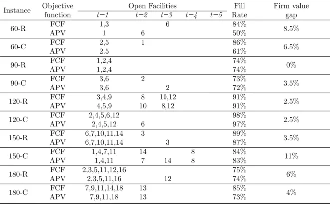
(ii) an exhaustive model whose objective function is the APV and with all constraints considered. For each instance, the network configurations ob-tained under F CF and AP V maximization are shown in Table 1. The first column of the table repre-sents the instance name, built from the number of customers and the coordinates pattern (R=random, C=clustered). The next five columns detail the list of facilities opened at each time period. The eight column represents the fill rate reached in the final period. In order to compare the FCF– and APV– driven solutions, we have a posteriori calculated the APV corresponding to solution obtained under FCF maximization. The percentage indicated in the ninth column represents the gap between both APVs. To get a more detailed picture of the model’s deci-sion mechanism, Figures 2 and 3 present the optimal network configurations for instance 150-C, obtained under FCF or APV maximization, respectively. The map represented in Figures 2 and 3 is divided into 3 markets standing for different economic param-eters. The markets are represented by different colors. As presented in table 1, maximizing FCF amount to open facilities 1,4,7 and 11 at period 1, facility 14 at period 2 and facility 8 at period 4. Maximizing APV amounts to select the same facilities at different time periods. The first reason for this difference is the im-pact of the tax shield benefit, which is higher in APV maximization. After opening facilities 1,4 and 11 at period 1, the company has used almost all its debt capacity. It still can open facility 7 in the first period using equity financing or open facility 7 at a later period using a larger debt capacity. The same mech-anism explains the more gradual network expansion under APV maximization.
The second reason is the time value of money, which is ignored by FCF. Opening facility 7 at period 2 rather than at period 1 as well as opening facility 14 at pe-riod 3 rather than at pepe-riod 2 leads to a lower fill rate (we recall that the firm is nonsensitive to the consumer’s behavior and that no back-order cost is
Figure 2 – Instance 150-C: network under FCF max-imization
Figure 3 – Instance 150-C: network under APV max-imization
MOSIM’20 - November 12-14, 2020 - Agadir - Morocco
Instance Objective Open Facilities Fill Firm value
function t=1 t=2 t=3 t=4 t=5 Rate gap
60-R FCF 1,3 6 84% 8.5% APV 1 6 50% 60-C FCF 2,5 1 86% 6.5% APV 2.5 61% 90-R FCF 1,2,4 74% 0% APV 1,2,4 74% 90-C FCF 3,6 2 73% 3.5% APV 3,6 2 72% 120-R FCF 3,4,9 8 10,12 91% 2.5% APV 4,5,9 10 8,12 91% 120-C FCF 2,4,5,6,12 98% 2.5% APV 2,4,5,12 6 97% 150-R FCF 6,7,10,11,14 3 89% 3.5% APV 6,7,10,11,14 3 87% 150-C FCF 1,4,7,11 14 8 84% 11% APV 1,4,11 7 14 8 83% 180-R FCF 2,3,5,11,12,16 75% 6% APV 2,3,5,11,16 12 74% 180-C FCF 7,9,11,14,18 13 85% 4% APV 7,9,11,18 13 73%
Table 1 – Network configuration under FCF and APV
assumed for unsatisfied customers), higher tax shield benefit and lower investment value due to the time value of money.
5 CONCLUSION
In this paper, we proposed an extension of traditional supply chain network models, driven by financial con-siderations. We propose to use the Adjusted Present Value (APV) as a performance indicator and show that this indicator enables decision makers to find a trade-off between logistic and financial priorities. The mathematical model is tractable by state of the art mixed integer linear programming solvers for realis-tic sizes of instances, opening perspectives for real-life applications. The numerical experiments show that using APV instead of traditional indicators does not bring considerable changes in the final configu-ration of the supply chain, but modifies its temporal implementation and can increase the firm value up to around 10%. Besides, focusing on the firm value rather on logistic costs tends to decrease the fill rate, i.e. the satisfaction of customers’ demand. Further research could aim at investigating the trade-offs be-tween the interest of various supply chain stakehold-ers.
ACKNOWLEDGMENT
This work has been supported by ANR under the FILEAS-FOG - ANR-17-CE10-0001 project.
Altman, E. I. (1968). Financial ratios, discrim-inant analysis and the prediction of corporate bankruptcy, The Journal of Finance, 23(4): 589-609.
Beaver, W. H. (1968). Market prices, financial ra-tios, and the prediction of failure, Journal of Ac-counting Research, 6(2): 179-192.
Damodaran, A. (2012). Investment valuation: Tools and techniques for determining the value of any asset, Vol. 666, John Wiley & Sons.
Hillegeist, S.A., Keating, E.K., Cram, D.P. and Lundstedt, K.G. (2004). Assessing the Prob-ability of Bankruptcy, Review of Accounting Studies,9,5-34.
Kallunki, J.-P. and Pyykk¨o, E. (2013). Do default-ing CEOs and directors increase the likelihood of financial distress of the firm?, Review of Ac-counting Studies, 18, 228-260.
La´ınez, J.M., Guill´en-Gos´albez, G., Badell, M, Es-pu˜na, A. and Puigjaner, L., (2007). Enhancing corporate value in the optimal design of chemical supply chains, Industrial & Engineering Chem-istry Research, 46(23): 7739-7757.
Leland, H. E. (1994). Corporate debt value, bond covenants, and optimal capital structure, The journal of finance, 49(4): 1213-1252.
Modigliani, F. and Miller, M. H. (1963). Corpo-rate income taxes and the cost of capital: a
cor-rection, The American economic review, 50(3): 433-443.
Myers, S. C. (1974). Interactions of corporate fi-nancing and investment decisions-implications for capital budgeting, The Journal of Finance, 29(1): 1-25.
Myers, S. C. (1984). The capital structure puzzle, The journal of finance, 39(3): 574-592.
Ramezani, M., Kimiagari, A. M. and Karimi, B. (2014). Closed-loop supply chain network de-sign: A financial approach, Applied Mathemat-ical Modelling, 38(15-16): 4099-4119.
Rezaei, H., Bostel, N., Hovelaque, V. and P´eton, O. (2020). An adjusted present value based supply chain network design model, Technical report, IMT Atlantique.
Shapiro, J. F. (2004). Challenges of strategic sup-ply chain planning and modeling, Computers & Chemical Engineering, 28(6-7): 855-861.