Learning Very Large Configuration Spaces: What Matters for Linux Kernel Sizes

HAL Id: hal-02314830

https://hal.inria.fr/hal-02314830

Submitted on 13 Oct 2019

HAL is a multi-disciplinary open access

archive for the deposit and dissemination of

sci-entific research documents, whether they are

pub-lished or not. The documents may come from

teaching and research institutions in France or

abroad, or from public or private research centers.

L’archive ouverte pluridisciplinaire HAL, est

destinée au dépôt et à la diffusion de documents

scientifiques de niveau recherche, publiés ou non,

émanant des établissements d’enseignement et de

recherche français ou étrangers, des laboratoires

publics ou privés.

Learning Very Large Configuration Spaces: What

Matters for Linux Kernel Sizes

Mathieu Acher, Hugo Martin, Juliana Pereira, Arnaud Blouin, Jean-Marc

Jézéquel, Djamel Khelladi, Luc Lesoil, Olivier Barais

To cite this version:

Mathieu Acher, Hugo Martin, Juliana Pereira, Arnaud Blouin, Jean-Marc Jézéquel, et al.. Learning

Very Large Configuration Spaces: What Matters for Linux Kernel Sizes. [Research Report] Inria

Rennes - Bretagne Atlantique. 2019. �hal-02314830�

Learning Very Large Configuration Spaces:

What Matters for Linux Kernel Sizes

Mathieu Acher

Univ Rennes Inria, CNRS, IRISA Rennes, France mathieu.acher@irisa.fr

Hugo Martin

Univ Rennes Inria, CNRS, IRISA Rennes, France hugo.martin@irisa.fr

Juliana Alves Pereira

Univ Rennes Inria, CNRS, IRISA Rennes, France juliana.alves- pereira@irisa.fr

Arnaud Blouin

Univ Rennes Inria, CNRS, IRISA Rennes, France arnaud.blouin@irisa.fr

Jean-Marc Jézéquel

Univ Rennes Inria, CNRS, IRISA Rennes, France jean- marc.jezequel@irisa.fr

Djamel Eddine Khelladi

CNRS, IRISA Rennes, France djamel- eddine.khelladi@irisa.fr

Luc Lesoil

Univ Rennes Inria, CNRS, IRISA Rennes, France luc.lesoil@irisa.fr

Olivier Barais

Univ Rennes Inria, CNRS, IRISA Rennes, France olivier.barais@irisa.fr

ABSTRACT

Linux kernels are used in a wide variety of appliances, many of them having strong requirements on the kernel size due to con-straints such as limited memory or instant boot. With more than ten thousands of configuration options to choose from, obtaining a suitable trade off between kernel size and functionality is an ex-tremely hard problem. Developers, contributors, and users actually spend significant effort to document, understand, and eventually tune (combinations of ) options for meeting a kernel size. In this paper, we investigate how machine learning can help explain what matters for predicting a given Linux kernel size. Unveiling what matters in such very large configuration space is challenging for two reasons: (1) whatever the time we spend on it, we can only build and measure a tiny fraction of possible kernel configurations; (2) the prediction model should be both accurate and interpretable. We compare different machine learning algorithms and demonstrate the benefits of specific feature encoding and selection methods to learn an accurate model that is fast to compute and simple to in-terpret. Our results are validated over 95,854 kernel configurations and show that we can achieve low prediction errors over a reduced set of options. We also show that we can extract interpretable in-formation for refining documentation and experts’ knowledge of Linux, or even assigning more sensible default values to options.

1

INTRODUCTION

With now more than 15,000 configuration options, Linux is one of the most complex configurable system ever developed in open source. If all these options were binary and independent, that would

This research was funded by the ANR-17-CE25-0010-01 VaryVary project. We thank Greg Kroah-Hartman (Linux foundation) and Tim Bird (Sony) for their support and the discussions. We also thank Paul Saffray, Alexis Le Masle, Michaël Picard, Corentin Chédotal, Gwendal Didot, Dorian Dumanget, Antonin Garret, Erwan Le Flem, Pierre Le Luron, Mickaël Lebreton, Fahim Merzouk, Valentin Petit, Julien Royon Chalendard, Cyril Hamon, Luis Thomas, Alexis Bonnet and IGRIDA technical support.

indeed yield 215000possible variants of the kernel. Of course not all options are independent (leading to fewer possible variants), but on the other hand some of them have tristate values: yes, no, or module instead of simply Boolean values (leading to more possible variants). Users can thus choose values for activating options – either compiled as modules or directly integrated within the kernel – and deactivate options. The assignment of a specific value to each option forms aconfiguration, from which a kernel can hopefully be compiled, built, and booted.

Linux kernels are used in a wide variety of systems, ranging from embedded devices, cloud services to powerful supercomputers [75]. Many of these systems have strong requirements on the kernel size due to constraints such as limited memory or instant boot. Obtaining a suitable trade off between kernel size, functionality, and other non-functional concerns (e.g., security) is an extremely hard problem. For instance, activating an individual option can increase the kernel so much that it becomes impossible to deploy it. Hubauxet al. [28] report that many Linux users complained about the lack of guidance for making configuration decisions, and the low quality of the advice provided by the configurators. Beyond Linux and even for much smaller configurable systems, similar configuration issues have been reported [4, 27, 63, 80, 82, 83, 86].

A fundamental issue is that configuration options often have a significant influence on non-functional properties (here: size) that are hard to know and modela priori. There are numerous possible options values, logical constraints between options, and potential interactions among configuration options [20, 33, 57, 60, 64] that can have an effect while quantitative properties such as size are themselves challenging to comprehend. As we will further elaborate in Section 2, the effort of the Linux community to document options related to kernel size is highly valuable, but mostly relies on human expertise, which makes the maintenance of this knowledge quite challenging on the long run.

Instead of a manual approach, we propose to follow an auto-mated approach based on statistical supervised learning: The idea is to build and measure a sample of kernel configurations and then use this sample to predict the properties (here: the size) of other con-figurations. The process of "sampling, measuring, learning" config-urations is obviously not novel, even in the context of configurable systems [20, 33, 57, 60, 64]. However, most of the works consider systems with a relatively low number of options (from dozens to hundreds). At the scale of Linux, some learning techniques are not applicable or suited for dealing with itsvery large configuration space: (1) whatever the time we spend on it, only a tiny fraction of possible kernel configurations can be built and measured; (2) there is a large number of options that can impact the prediction. Another related problem is that we want to extractinterpretable information that can be communicated to developers and users of Linux. High accuracy is of course important but interpretability of the prediction model is also a prime concern. The complexity of the Linux configuration space changes the perspective and raises several unaddressed questions: How many configurations should be measured to reach a high accuracy? Do all configuration options have an effect on size? Can automated learning retrieve or even supplement Linux community knowledge about options?

Our key contribution is to unveil"what matters" within the very large configuration space of Linux. To do so, we first need to iden-tify what does matter for instrumenting the learning process and reaching a good enough accuracy —which measures of sizes, which strategies to engineer features, which machine learning algorithms, etc. We develop specific feature engineering techniques to select a subset of relevant options. We empirically show that feature selec-tion can be applied to improve training time, interpretability and accuracy of the prediction. Thanks to interpretable information, we can identify what options matter w.r.t. kernel size and validate our findings. We confront our discovered influential options with Linux documentation, pre-defined configurations (tinyconfig), and experts’ knowledge. We show that a large portion of identified options does have an explanation. Our results open the way for im-proving Linux documentation, specifying default values of options, and guiding users when configuring the kernel. We validate our results over 95,854 configurations using different measures (binary size, compressed sizes).

The contributions of this paper are as follows:

• The design and implementation of a large study about ker-nels’ sizes. We describe opportunities to compute at scale different measures and we engineer specific methods for feature encoding, selection, and construction;

• A comparison of a wide range of machine learning algo-rithms and the effects of feature engineering over (1) predic-tion errors and (2) interpretability. We analyse the amount of configurations needed for training and replicate the ex-periments using different measures of kernel size. We find that it is possible to identify a reduced set of options that influence size using a relatively small samplei.e., we identify "what matters" when predicting;

• A qualitative analysis of identified options based on the cross-analysis of Linux documentation, default options’ values and configurations, and experts’ knowledge. We find that "what

matters" is either coherent or can be used to refine Linux knowledge;

• A comprehensive dataset of 95,854 configurations with 19 measurements of sizes as well as learning procedures for replication and reproducibility of the results [70].

With respect to the categorized research methods by Stol et al. [69], our paper mainly contributes to a knowledge-seeking study. Specif-ically, we perform a field study of Linux, a highly-configurable system and mature project. We gain insights about kernels’ proper-ties using a large corpus of configurations. Our contribution is also a solution-seeking study since we develop techniques for configu-ration measurements, feature engineering and machine learning to predict size in an accurate yet interpretable way.

Audience. The intended audience of this paper includes but is not limited to Linux contributors. Researchers and practitioners in configurable systems shall benefit from our learning process and insights. We also provide evidence that machine learning is applicable for very large space of software configurations.

2

SIZE MATTERS

2.1

Linux, options, and configurations

The Linux kernel is a prominent example of a highly-configurable system. Thousands of configuration options are available on differ-ent architectures (e.g., x86, amd64, arm) and documented in several Kconfig files. For the x86 architecture and the version 4.13.3, de-velopers can use 12,797 options to tailor (non-)functional needs of a particular use (e.g., embedded system development). The ma-jority of options has either boolean values (‘y’ or ‘n’ for activat-ing/deactivating an option) or tri-state values (‘y’, ‘n’, and ‘m’ for activating an option as a module). There are also numerical or string values. Options may have default values. Because of cross-cutting constraints between options, not all the combinations of values are possible. For example, Figure 1 depicts the KConfig file that describes theLOCK_STAT option. This option has several direct de-pendencies (e.g., LOCKDEP_SUPPORT ). When selected, this option activates several other options such asLOCKDEP. By default, this option is not selected (’n’). As a case in point, this option documen-tation (help part) gives no indication to a beginner user about the impact of the option on the kernel size.

config LOCK_STAT

bool "Lock usage statistics"

depends on STACKTRACE_SUPPORT && LOCKDEP_SUPPORT ... select LOCKDEP

select DEBUG_SPINLOCK ... default n

help

This feature enables tracking lock contention points. For more details, see Documentation/locking/lockstat.txt This also enables lock events required by "perf lock", subcommand of perf. If you want to use "perf lock", you also need to turn on CONFIG_EVENT_TRACING. CONFIG_LOCK_STAT defines "contended" and "acquired" lock events. (CONFIG_LOCKDEP defines "acquire" and "release" events.)

Figure 1: Option LOCK_STAT (excerpt)

Users of the Linux kernel set values to options (e.g., through a configurator [81]) and obtain a so-called.config file. We consider that aconfiguration is an assignment of a value to each option. Based on a configuration, the build process of a Linux kernel can

start and involves different layers, tools, and languages (C, CPP, gcc, GnuMake and Kconfig).

2.2

Use cases and scenarios

There are numerous use-cases for tuning options related to size in particular [26, 53]:

• the kernel should run on very small systems (IoT) or old machines with limited resources;

• Linux can be used as the primary bootloader. The size re-quirements on the first-stage bootloader are more stringent than for a traditional running operating system;

• size reduction can improve flash lifetime, spare RAM and maximize performances;

• a supercomputing program may want to run at high perfor-mance entirely within the L2 cache of the processor. If the combination of kernel and program is small enough, it can avoid accessing main memory entirely;

• the kernel should boot faster and consume less energy: though there is no empirical evidence for how kernel size relates to other non-functional properties (e.g., energy con-sumption), practitioners tend to follow the hypothesis that the higher the size, the higher the energy consumption. • cloud providers can optimize instances of Linux kernels w.r.t.

size;

• in terms of security, the attack surface can be reduced when optional parts are not really needed.

When configuring a kernel, size is usually neither the only con-cern nor the ultimate goal. The minimization of the kernel size has no interest if the kernel is unable to boot on a specific device. Size is rather part of a suitable tradeoff between hardware constraints, functional requirements, and other non-functional concerns (e.g., security). The presence of logical constraints and subtle interactions between options further complicates the task.

To better understand how size is managed in the Linux project, we look at the Linux documentation, tiny kernel pre-defined con-figuration, and Linux community knowledge. Next, we describe these sources of information. Later, we will use this information to validate our proposal.

2.3

Kernel Sizes and Documentation

We first conducted a study that identifies the kernel options for which the documentation explicitly discusses an impact on the kernel size. We apply the following method.

Protocol. The objects of the study are the KConfig files that describe and document each kernel option. We use theKConfigLib tool to analyze the documentation of the Linux kernel 4.13.3 for the x86 architecture [25]. This architecture contains 12,797 options. The first step of this analysis consists in automatically gathering the options whose documentation contains specific terms related to size terminology:big, bloat, compress, enlarge, grow, huge, increase, inflat, inlin, larger, little, minim, optim, overhead, reduc, shrink, size, small, space, trim, percent and size values (e.g., 3%, 23 MB). The list of terms was built in an iterative way: we intensively read the documentation and checked whether the terms cover relevant options, until reaching a fixed point. The second step of this analysis consists of manually scrutinizing each such KConfig documentation

to state whether it indeed discusses a potential impact of the option on the kernel size. A first person did this task. The results were double-checked by a second person. These two persons are authors of this paper with no background on the Linux kernel to make sure that the identified options are explicitly (and not implicitly or learned by previous experience) referring to the kernel size.

Results. On the 12,797 options, 2,233 options have no documen-tation (17.45%). We identified 147 (1.15%) options thatexplicitly discuss potential effects on the kernel size. Kernel developers use quantitative or approximate terms to describe the impact of options on the kernel size.

Quantitative examples include: "will reduce the size of the driver object by approximately 100KB"; "increases the kernel size by around 50K"; "The kernel size is about 15% bigger".

Regarding approximate terms, examples include: the "kernel is significantly bigger"; "making the code size smaller"; "you can dis-able this option to save space"; "Disdis-able it only if kernel size is more important than ease of debugging".

2.4

Tiny Kernel Configuration

The Linux community has introduced the commandmake tiny-config to produce one of the smallest kernel possible. Though it does not boot on anything, it can be used as a starting point fore.g., embedded systems in efforts to reduce kernel size. Technically, it starts fromallnoconfig that generates a kernel configuration with as many options as possible set to’n’ values. allnoconfig works as follows: Following the order of options in the KConfig files, a greedy algorithm iteratively sets’n’ values to options. Due to numerous constraints among options and throughout the process, other de-pendent options may be set to’y’ values. In a second and final step, options’ values of Figure 2 override the values originally set by allno-config. For example, the value of CONFIG_CC_OPTIMIZE_FOR_SIZE can be set to ’y’ (overriding its original value ’n’).

# CONFIG_CC_OPTIMIZE_FOR_PERFORMANCE is not set CONFIG_CC_OPTIMIZE_FOR_SIZE=y

# CONFIG_KERNEL_GZIP is not set # CONFIG_KERNEL_BZIP2 is not set # CONFIG_KERNEL_LZMA is not set CONFIG_KERNEL_XZ=y

# CONFIG_KERNEL_LZO is not set # CONFIG_KERNEL_LZ4 is not set CONFIG_OPTIMIZE_INLINING=y # CONFIG_SLAB is not set # CONFIG_SLUB is not set CONFIG_SLOB=y

CONFIG_NOHIGHMEM=y

# CONFIG_HIGHMEM4G is not set # CONFIG_HIGHMEM64G is not set

Figure 2: Pre-set values of tinyconfig for X86_64 architecture. As far as possible, other options are set to ’n’ values.

Experts of the Linux project have specified options of Figure 2 based on their supposed influence on size. Specifically, _{CONFIG_CC_OPTIMIZE_FOR_SIZE} calls the compiler with the −Os flag instead of −O2 (as with CONFIG_CC_OPTIMIZE_FOR_PERFORMANCE). The option CONFIG_KERNEL_XZ is the compression method of the Linux kernel:tinyconfig relies on XZ instead of GZIP (the default choice). CONFIG_OPTIMIZE_INLINING option determines if the kernel forces gcc to inline the functions developers have marked ’inline’.

CONFIG_SLOB is one of three available memory allocators in the Linux kernel. Finally,CONFIG_NOHIGHMEM, CONFIG_HIGHMEM4G, or CONFIG_HIGHMEM64G set the physical memory on x86 systems: the option chosen here assumes that the kernel will never run on a machine with more than 1 Gigabyte total physical RAM.

We will revisit the strategy oftinyconfig in Section 5.

2.5

Community attempts

We review (informal) initiatives in the Linux community that are dealing with kernel sizes.

The Wiki https://elinux.org/Kernel_Size_Tuning_Guide provides guidelines to configure the kernel and points out numerous impor-tant options related to size. However the page is no longer actively maintained since 2011. Tim Bird (Sony) presented "Advanced size optimization of the Linux kernel" in 2013. Josh Triplett (Intel) intro-ducedtinyconfig at Linux Plumbers Conference 2014 ("Linux Kernel Tinification") and described motivating use-cases. The leitmotiv is to leave maximum configuration room for useful functionality while exploiting opportunities to make the kernel as small as possi-ble. It led to the creation of the project http://tiny.wiki.kernel.org. The last modifications were made 5 years ago on Linux versions 3.X https://git.kernel.org/pub/scm/linux/kernel/git/josh/linux.git/. Pieter Smith (Philips) gave a talk about "Linux in a Lightbulb: How Far Are We on Tinification (2015)". Michael Opdenacker (Bootlin) described the state of Linux kernel size in 2018. Accord-ing to these experts, techniques for size reduction are broad and related to link-time optimization, compilers, file systems, strippers, etc. In many cases, a key challenge is that configuration options spread over different files of the code base, possibly across subsys-tems [2, 3, 6, 44, 47, 55, 56].

2.6

Problem summary and approach

Use cases, Kconfig documentation, options values for default con-figurations, as well as past and ongoing initiatives provide evidence that options related to kernel size are an important issue for the Linux community. However, the human effort to document config-uration options and maintain the knowledge over time and kernel evolutions is highly challenging. It is actually a well-known phe-nomenon reported for many software systems [63] that is due to the exponential number of possible configurations.

A more automated approach could thus be helpful to capture the essence of size-related options in the very large configuration space of Linux. Since building all configurations is infeasible, our idea is to learn from a sample of measured configurations. The goal is to predict the effects of options w.r.t. size in such a way that users can then make informed and guided configuration decisions.

We should thus strive for the right balance betweenaccuracy (our prediction is close enough to reality) andinterpretability, because we want to communicate to developers and users which options matter for the kernel size. Users in charge of configuring the kernel should indeed have the maximum of flexibility to meet their specific requirements (directly related to size or not).

3

FROM MEASURING TO PREDICTING

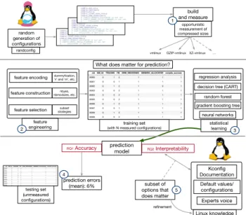
This section presents the end-to-end process we used to learn from a sample of configuration measurements. We detail each step of

random generation of configurations randconfig build and measure opportunistic measurement of compressed sizes

vmlinux GZIP-vmlinux XZ-vmlinux …

feature encoding

feature selection feature construction

neural networks decision tree (CART)

random forest gradient boosting tree

regression analysis statistical learning feature engineering prediction model RQ1 Accuracy RQ2Interpretability Kconfig Documentation Default values/ configurations Linux knowledge about options Experts voice prediction errors (mean): 6% training set (with N measured configurations)

testing set (unmeasured configurations) subset of options that does matter dummyfication, ’n’ and ‘m’, etc. nbyes, nbmodules, etc. subset strategies 1 2 3 5 refinement

What does matter for prediction?

4

Figure 3: Design study and technical infrastructure for mea-suring and predicting configurations.

Figure 3, highlighting the innovative details (if any). This section should also be read as the design of an experimental study that aims to understand how the different steps affect the outcomei.e., prediction errors and interpretability.

3.1

Measuring at scale

The first step is to measure kernel sizes from configurations. We used TuxML, a tool to build the Linux kernel in the largei.e., what-ever options are combined. TuxML relies on Docker to host the numerous packages needed to compile and measure the Linux kernel. Docker offers a reproducible and portable environment – clusters of heterogeneous machines can be used with the same libraries and tools (e.g., compilers’ versions). Inside Docker, a col-lection of Python scripts automates the build process. A first step is the selection of configurations to build. We rely onrandconfig to randomly generate Linux kernel configurations (see the top of Fig-ure 3).randconfig has the merit of generating valid configurations that respect the numerous constraints between options. It is also a mature tool that the Linux community maintains and uses [44]. Thoughrandconfig is not producing uniform, random samples (see Section 6), there is a diversity within the values of options (being ’y’, ’n’, or ’m’). Given.config files, TuxML builds numerous kernels. Throughout the process, TuxML can collect various kinds of infor-mation, including the build status and the size of the kernel. We concretely measurevmlinux, which is a statically linked executable file that contains the kernel in object file format.

3.2

Opportunistic measurements

For creating a bootable image, the kernel is also compressed. Config-uration options (e.g., CONFIG_KERNEL_GZIP) are employed to select a compression method: GZIP (default), BZIP2, LZMA, LZO, LZ4, or XZ (default fortinyconfig, see Listing 2). Strictly speaking, the measurement of a specific compressed size requires to build and

measure a new fresh configuration with the related options acti-vated. However the building process is very costly and took more than 9 minutes per configuration on average (standard deviation: 11 min). So instead of compiling from scratch a configuration, we use the following trick: Once we finished the build of a given con-figuration, we compile again the kernel by just changing options related to compression. We notice that the compression operates at the end of the build process andmake command is smart enough to not recompile the whole code source. Looking at Listing 2, we can activate_{CONFIG_KERNEL_LZMA (says) and deactivate other} compres-sions’ options. In fact, we did that for the 6 compression methods. Almost for free, we get 18 additional size measurements of kernel configurations (calledGZIP-vmlinux, XZ-vmlinux, ... in Figure 3).

3.3

Feature engineering

Predicting the size of a kernel (beingvmlinux or a compressed kernel) is a supervised, regression problem. Out of a combination of options values (i.e., a configuration), the learning model should be able to predict a quantitative value (the size) without actually building and measuring the kernel. We have at our disposal asample ofd measurements S = {(c1, s1), (c2, s2), . . . , (c_d, s_d)} (c_idenoting a

configuration, ands_idenoting the size of it) over the (unknown) full set of configurations C. The goal is to learn an accurate regression modelf that can predict the performance of Linux configurationsˆ given a small number of observations S ⊂ C. Specifically, we aim to minimize the prediction error over the whole configuration space of Linux: arg min

c ∈C\S

L(f (c), ˆ f (c))

whereL is a loss function to penalize errors in prediction and f the actual function in charge of measuring sizes.

The way the problem is represented is crucial for machine learn-ing algorithms and depends on an adequate set of features to train on. In our case, features are mostly configuration options of Linux but there are also opportunities to discard irrelevant values or fea-tures. We now explain how we encode features, what new features we create, and strategies to select a relevant subset of features (see step 2 of Figure 3).

3.3.1 Feature encoding. Regression analysis requires that we en-code possible values of options (e.g.,’y’, ’n’, ’m’) into numerical values. An encoding of ’n’ as 0, ’y’ as 1, and ’m’ as 2 is a first possible solution. However, some learning algorithms (e.g., linear regression) will assume that two nearby values are more similar than two distant values (here ’y’ and ’m’ would be more similar than ’m’ and ’n’). This encoding will also be confusing when in-terpreting the negative or positive weights of a feature. There are many techniques to encode categorical variables (e.g., dummy vari-able [13]). We observe that the ’m’ value has no direct effect on the size since kernel modules are not compiled into the kernel and can be loaded as needed. Therefore, we consider that ’m’ values have the same effect as ’n’ values and values can be merged. As a result, the problem is simplified:an option can only take two values ("yes" or "not yes"). With this encoding, the hypothesis is that the accuracy of the prediction model is not impacted whereas the problem is simpler to handle for learning algorithms and easier to interpret. 3.3.2 Feature construction. The number of ’y’ values in a configu-ration, denoted#yes, can have an impact on the kernel size. The

rationale is that the more options are included, the larger is the kernel. Similarly, we can consider features like#no or nbmodule. By adding such features, the hypothesis is that the accuracy of the prediction model can be improved.

3.3.3 Feature selection. A hypothesis is that some configuration options have little effects and can be removed without incurring much loss of information. Feature selection techniques are worth considering when there are many features and comparatively few samples. Though we are not necessarily in extreme cases like the analysis of DNA microarray data [68], we can consider scenarios in which the number of configurations in the training set is (much) less than 10K. In any case, selecting a subset of relevant features have several promises: simplification of models to make them easier to interpret; shorter training times; enhanced accuracy. As a side note, we do not use feature extraction (e.g., principal component analysis) that derivesnew features out of existing ones. We prefer to identify a subset of existing options that can be directly understood and discussed.

There are several methods to perform feature selection. A first approach is to remove features with low variance. In our case, we remove options that have a unique value (e.g., always ’y’ value). To identify the best features, it is also possible to apply univariate statistical tests (e.g., F-score). The principle is to test the individual effect of each option on size (e.g., the degree of linear dependency). Another method is to use a predictive model (e.g., Lasso or a deci-sion tree) to remove unimportant features. A threshold should be determined to account how many features should be considered as important. Finally, some learning algorithms perform feature selection as part of their overall operatione.g., Lasso penalizes the regression coefficients with an L1 penalty, shrinking many of them to zero [74].

As far as possible, we consider all these strategies as part of our experiments. As a baseline, we also try with domain knowledge coming from Linux documentation. The overall goal is to find a good tradeoff between computational complexity, informative and reduced feature set, and prediction error.

3.4

Statistical Learning

Once the data is well represented, it is time to learn out of a training set (see step 3 of Figure 3). There are many algorithms capable of handling a regression problem. We have consideredlinear methods for regression, decision trees (CART), random forests, gradient boost-ing trees, and neural networks [18]. These algorithms differ in terms of computational cost, expressiveness and interpretability. For in-stance, linear regressions are easy to interpret, but are unable to capture interactions between options and handle non-linear effects. On the opposite side of the spectrum, neural networks are hard to interpret but probably can reach high accuracy. In between, there are variants of algorithms (e.g., Lasso) or families of algorithms (e.g., random forests). We chose to work with this set of algorithms since (1) they have already been successfully used in the literature of configurable systems [57];(2) we aim to gather (strong) baselines and find a good tradeoff w.r.t. accuracy and interpretability.

3.4.1 Hyperparameters. Most of the selected algorithms are highly sensitive to hyperparameters, which may have effects on results. We explore a wide range of values as part of our study [70]. 3.4.2 Feature importance. Knowing which options are most pre-dictive of size is part of our goal. In this respect, feature importance is a useful concept: It is the increase in the prediction error of the model after we permuted the feature’s values [46]. For decision tree, the importance of a feature is computed as the (normalized) total reduction of the splitting criterion (e.g., Gini or entropy) brought by that feature. For random forest, we measure the importance of a feature by calculating the increase in the model’s prediction error afterpermuting the feature [7, 46].

4

EXPERIMENT STUDY

We address two main research questions:

•(RQ1) How accurate is the prediction model? Depend-ing one.g., training set size, feature selection or hyperpa-rameters of learning algorithms, the resulting model may produce more or fewer errors when predicting the size of unseen configurations.

•(RQ2) How interpretable is the prediction model? Do the identified options explain the effect on kernel size and can we learn from them? Similarly as RQ1, different factors (aka independent variables) of our study may affect the quality of the interpretable information we can extract from the model. Though the two research questions have similar independent variables (see step 4 and 5 in Figure 3), we need to use different methods and metrics to answer RQ1 and RQ2.

4.1

Metric for prediction error

Several metrics and loss functions can be considered for comput-ing accuracy. For presentcomput-ing and comparcomput-ing results, we rely on the mean absolute percentage error (MAPE) defined as follows: MAPE=100 t Ít i=1   f(ci)− ˆf (ci)    f (ci) %

We choose MAPE since (1) it is frequently used when the quan-tity to predict is known to remain above zero (as in our case); (2) it has the merit of being easy to understand and compare (it is a percentage); (3) it handles the wide distribution and outliers of vm-linux size (Figure 4); (4) it is commonly used in approaches about learning and configurable systems [57]. We split our sample of 95,854 configurations and their associated performance measures into a training and a testing set. The training set is used to obtain a prediction model, while the testing set is used to test its predic-tion performances through the MAPE. The principle is to confront predicted values (f (cˆ _i)) to observed values (f (c_i) – ground truth).

4.2

Assessment of interpretability

There is neither a mathematical definition of interpretability nor a universal metric for quantifying it. In our context, we consider that the interpretability is the ability of a learning process to reveal what configuration options matter for predicting size. In the ab-sence of ground truth (see Section 2), we seek to find evidence that can justifywhy options are considered as important. This question can only be treated with qualitative methods (though automated

techniques can partly ease the task). Hence, we confront our ranked list of important features with Linux knowledge (e.g., Kconfig docu-mentation) and seek to find explanations about their effects on size. Two authors of the paper made the effort and discussed their analy-sis until reaching an agreement. We also exchanged with two Linux experts through emails for clarifying the effects of some options.

4.3

Implementation

We rely on Python modules scikit-learn [8] to benefit from state of the art machine learning algorithm implementation. We also build an infrastructure around these libraries to automatically handle the feature engineering part, the control of hyperparameters, training set size,etc. For example, it is possible to specify a range of values in order to exhaustively search the best hyperparameters for a given algorithm (more details can be found online [70]). Technically, the infrastructure created is a Docker image [70] that takes a configu-ration file as input (including the specification ofe.g., training set size, feature selection method) and serializes the results for further analysis (e.g., MAPE and feature importance). This approach will make it easy to reproduce all our experiments at scale.

For the implementation of the neural network, we rely on Tensor-flow [1]. The neural network is a multilayer feed forward network. The input layer takes a set of features: for each feature, every con-figuration is either 1 = "activated" if the feature is activated in the kernel configuration or 0 = "not activated" if not, as described in Sec-tion 3.3.1. Then these configuraSec-tions go through three dense layers with ReLU activation functions. The output is the predicted size of the kernel (compressed or not). The loss metric we use is MAPE, as defined in Section 4.1. We rely on an Adam Optimizer (in our case, it had better convergence properties in comparison to a standard stochastic gradient descent). We first launch 15 initialization steps with a high learning rate (around 0.5, to reach a local minimum with few steps). Then, we launch 15 more accurate steps, with a lower learning rate (0.025). We split the dataset into a training and a testing set, feed the network with batches of 50 configurations of the training set, predict the size of the testing set and compare it with the measured size of the testing set. Besides, we noticed that the architecture of the neural network should be revised for small training sets. Specifically, when the size of the training set is lower than 1000 configurations, we chose a monolayer (which is basically a linear regression with a ReLU activation). When the size of the training set is between 1 and 10 thousands configurations, we chose a 2-layers architecture.

Instrumentation. We vary the training size with N ∈ {10, 20, ..., 90} a percentage of the total set. To mitigate the random selection of the training set, we have repeated the experiments 10 times and report the average and standard deviation for all algo-rithms.

4.4

Dataset

We only focus on the kernel version 4.13.3 (release date: 20 Sep 2017). It is a stable version of Linux (i.e., not a release candi-date). Furthermore, we specifically target the x86-64 architecture i.e., technically, all configurations have values CONFIG_X86=y and CONFIG_X86_64=y.

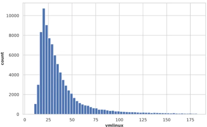
0 25 50 75 100 125 150 175 vmlinux 0 2000 4000 6000 8000 10000 count

Figure 4: Distribution of size (in Mb) without outliers

During several months, we used a cluster of machines to build and measure 95,854 random configurations. In total, we invested 15K hours of computation time. We removed configurations that do not build (e.g., due to configuration bugs of Linux). The number of possible options for x86 architecture is 12,797 options, but the 64 bits further restricts the possible values (some options are always set to ’y’ or ’n’ values). Furthermore,randconfig does not vary all options values. We observe that more than 3,000 options have a unique value. We use this opportunity to remove them; it can be seen as a straightforward and effective way of doing feature selection. Overall, 9,286 options have more than one valuei.e., there are nine thousand predictors that can potentially have an effect on size. Each configuration is composed of 9,286 options together with 13 measurements (vmlinux, and vmlinux compressed with 6 methods). Overall the dimension of the configuration matrix is 9,286 x 95,854.

5

RESULTS

Before discussingRQ1 and RQ2, we present two key results of our dataset.

Size distribution. The minimum size of vmlinux is 7Mb and roughly corresponds to the size oftinyconfig. The maximum is 1,698.14Mb, the mean is 47.35Mb with a standard deviation of 67Mb. Figure 4 shows the distribution of vmlinux size (with 0.97 as quantile for avoiding extreme and infrequent values of sizes). Most values are around 25Mb, and there is an important variability in sizes.

Compressed sizes and vmlinux. We compute the Pearson cor-relations between the size of vmlinux and the size of compressed kernels. On average, the correlation is moderate (+0.53) with almost no variation. For instance, the correlation betweenGZIP-vmlinux andvmlinux is 0.52. On a more positive note, the compressed sizes are highly correlated to each other (+0.99 on average, std≈ 0). The consequence of these results is that(1) two prediction models should be built (one for compressed size, one forvmlinux); (2) one prediction model for one compressed size is sufficient. In the re-minder, we reported the results forvmlinux and briefly describe the results for compressed sizes (more details can be found online [70]).

5.1

(RQ1+RQ2) Effects of feature engineering

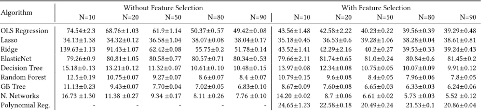
Let us start with the following setting: the use of ordinary least squares (OLS) for linear regression together with a naive feature encoding of categorical features (as described in Section 3.3.1). It leads up to MAPE=4,000% for N=90% of the training set. The result is much better when the values ’n’ and ’m’ are equally encoded: OLS gives MAPE=75% for N=90%.

We observe similar improvements with shrinkage-based linear regression. The improvement is less spectacular with tree-based methods or neural networks, but the accuracy remains slightly bet-ter with the encoding.A first conclusion is that the feature encoding that mixes ’module’ and ’no’ values is well-suited, w.r.t. accuracy. By construction, it has also the merit of simplifying the problem; we will use it in the remainder.

The inclusion of new features that count the number of ’y’, ’n’, and ’m’ values gives interesting insights. The linear correlation be-tween_{#yes and}vmlinux is weak: Pearson coefficient is 0.19. Lasso, Ridge, or ElasticNet, under some hyperparameters values, can only keep 2 features with non-zero coefficients:_{DEBUG_INFO, and #yes.} In other words, these algorithms tend to shrink too many coeffi-cients under the profit of_{#yes. The non-inclusion of #yes or a} different hyperparameter tuning allows Lasso, Ridge or ElasticNet to identify much more relevant features with non-zero coefficients, thus improving their own MAPE and providing more interpretable information. For decision trees, random forests and gradient boost-ing trees,_{#yes is a very strong predictor. This feature is ranked} in the top 3 forvmlinux and GZIP-vmlinux. We also observe im-provements of MAPE when_{#yes is part of the feature selection.} We conclude that #yes (1) should be used with caution ( e.g., for fea-ture selection), (2) other options can potentially compensate its effect for reaching similar accuracy, but it requires the use of much more features as part of feature selection (3) it has high importance w.r.t. interpretability. The use of #yes has several interests, and we will use it in the remainder, except for Lasso, Ridge, and ElasticNet given that the inclusion of_{#yes aggressively shrinks too many} coefficients.

5.2

(RQ1) Accuracy

In Table 1, we report the MAPE (and its standard deviation) of multiple statistical learning algorithms, on various training set sizes (N), with and without feature selection1.

We observe that Algorithms based on linear regression (Lasso, Ridge, Elasticnet) do not work well, having a MAPE of more than 30% whatever the training set size of the feature selection. Some does not even take advantage of a bigger training set, like Lasso which is even increasing its MAPE from 34% to 38% when the train-ing set size goes from 10% to 90%. Tree-based algorithms (Decision Tree, Random Forest, Gradient Boosting Tree) tend to work far better (MAPE of 15% and lower) and effectively take advantage of more data to train on. As a base of comparison, we also report results from Neural Networks which are better than other algo-rithms when fed with a big enough training set. Note that without feature selection, Random Forest and Gradient Boosting Tree are

1

For this experiment we used a very crude feature selection, based on the ordering yield by a random forest trained on a subset of dataset, where every feature was present.

Algorithm

Without Feature Selection With Feature Selection

N=10 N=20 N=50 N=80 N=90 N=10 N=20 N=50 N=80 N=90 OLS Regression 74.54±2.3 68.76±1.03 61.9±1.14 50.37±0.57 49.42±0.08 43.56±1.48 42.58±2.22 40.23±0.22 39.56±0.39 39.29±0.48 Lasso 34.13±1.38 34.32±0.12 36.58±1.04 38.07±0.08 38.04±0.17 35.18±0.45 36.53±0.6 39.28±1.06 38.28±0.04 38.61±0.81 Ridge 139.63±1.13 91.43±1.07 62.42±0.08 55.75±0.2 51.78±0.14 43.52±1.41 42.29±2.16 40.2±0.27 39.53±0.33 39.24±0.43 ElasticNet 79.26±0.9 80.81±1.05 80.58±0.77 80.57±0.71 80.34±0.53 79.66±2.11 81.74±0.65 81.0±0.24 80.84±0.6 81.45±0.2 Decision Tree 15.18±0.13 13.21±0.12 11.32±0.07 10.61±0.10 10.48±0.15 13.97±0.08 12.34±0.08 10.75±0.05 10.07±0.09 9.91±0.12 Random Forest 12.5±0.19 10.75±0.07 9.27±0.07 8.6±0.07 8.4±0.07 10.79±0.15 9.6±0.08 8.4±0.05 7.96±0.06 7.8±0.05 GB Tree 11.13±0.23 9.43±0.07 7.70±0.04 7.02±0.05 6.83±0.10 8.67±0.09 7.60±0.08 6.65±0.03 6.33±0.03 6.24±0.06 N. Networks 16.73±1.30 11.38±0.27 9.34±0.17 8.11±0.26 7.76±0.10 14.20±0.02 8.7±0.06 6.61±0.02 5.73±0.03 5.52±0.12 Polynomial Reg. - - - 24,65±1.23 22.58±0.18 20.49±0.24 21.53±0.1 20.86±0.04

Table 1: MAPE of different learning algorithms for the prediction of vmlinux size, without and with feature selection

better than Neural Networks, and with feature selection, Gradient Boosting Tree is even competitive up to when 50% of the dataset is used as a training set. Polynomial Regression does not scale without feature selection, and even with feature selection, only reaches a MAPE of 20% at best.

Figure 5 aims to show the influence on the accuracy of (1) the numberk of selected features and (2) the training set percentage (N) of the full dataset. In particular, it depicts how random forest performs when varyingk and N. We observe that for a training set size of N=10% (9,500), the accuracy peaks (i.e., lowest errors rate) whenk=200 with a MAPE of 10.45, and consistently increases with more columns. For a training set size of N=50% (47,500), accuracy peaks whenk=200 with a MAPE of 8.33. For N=90% (85,500), we reach a MAPE of 7.81 withk=250. Independently from the training set size, we consistently observe in Figure 5 that the MAPE is the lowest whenk is in the range 200—300. This optimal number of selected features is similar with Gradient Boosting Tree and also exists for every algorithm, although it can change from one algorithm to another. For example, for Ridge or ElasticNet, it is in the range 250—300, for Lasso, 350—400, and for Neural Networks, 400—500. In Table 1 are reported the results with feature selection of the optimal number for each algorithm.

Given these results, we can say that out of the thousands of options of Linux kernel, only a few hundred actually influence its size. From the machine learning point of view, the other columns do not bring any more information and even make the model worse by biasing it.

Results of compressed sizes. We report better accuracy when predictingGZIP-vmlinux for all algorithms and training set size. Random forests can quickly reach 6% of prediction errors (for N=10% and without feature selection). Neural networks can even get a MAPE of 2.8% (for N=90% and with feature selection). We also observe that feature selection pays off: only a few options (≈ 200) are needed to get competing results [70].

We find a sweet spot where only 200—300 features are suf-ficient to efsuf-ficiently train a random forest and a Gradient Boosting Tree to obtain a prediction model that outper-forms other baselines (7% prediction errors for 40K config-urations). We observe similar feature selection benefits for any training set size and tree-based learning algorithms.

Figure 5: Evolution of MAPE w.r.t. the number k of selected features and the training set percentage N (random forest).

5.3

(RQ2) Interpretability

Contrary to Neural networks, Gradient Boosting Tree or Random Forest are algorithms with built-in explainability. There we can extract a list of features that can be ordered by their importance with respect to the property of interest (here size). So the question is: how does this ordered list of features relate to reality?

Confrontation with documentation. We confront the or-dered list of features yield by Random Forest to the 147 options referring to size in the Kconfig documentation (see Section 2.3). First, we notice that 31 options have a unique value in our dataset: randconfig was unable to diversify the values of some options and therefore the learning phase cannot infer anything. We see it as an opportunity to further identifying influential options. As a proof of concept, we sample thousands of new configurations with and without optionKASAN_INLINE activated (in our original dataset, KASAN_INLINE was always set to ’n’). We did observe size increase (20% on average). We have also tried for 5 other options and did not observe a significant effect on size [70].

Among the resulting 116 options (147− 31), we found that: • 11 are in the top 200, 7 are in the top 200—500, and 5 in the

top 500—1000: 15% of options are in the sweet spot of our feature selection (see RQ1);

• 67% of remaining options are beyond the rank 2000. We iden-tified two patterns of explanations. First, the effect on size is

simply negligible: It is explicitly stated as such in the docu-mentation ("This will increase the size of the kernelcapi module by 20 KB" or "Disabling this option saves about 300 bytes"). Second, some options’ values are not frequent enough (e.g., 98% ’y’ and 2% ’n’ value): most probably, the learning phase needs more diverse instances. Again, we see the KConfig documentation as an opportunity to guide the sampling of the configuration space and further find influential options. Finding of undocumented options. A consequence from the confrontation with KConfig is that the vast majority of influential options is either not documented or not referring to size. In order to further understand this trend, we analyze the top 50 options corresponding to the 50 first features yield by Random Forest:

• only 7 options are documented as having a clear influence on size;

• our investigation and exchanges with domain experts show that the 43 remaining options are either (1) necessary to ac-tivate other options; (2) the underlying memory used would be based on the size of the driver; (3) chip-selection configu-ration (you cannot run the kernel on the indicated system without this option turned on); (4) related to compiler cov-erage instrumentation, which will affect lots (possible all) code paths; (5) debugging features

Revisiting tinyconfig. In our dataset, we observe that tiny-config is by far the smallest kernel (≈7Mb). The second smallest configuration is≈11Mb. That is, despite 90K+ measurements with randconfig, we were unable to get closer to 7Mb. Can our prediction model explain this significant difference (≈4Mb)?

A first hypothesis is that pre-set options have an important impact on the size (see Figure 2, page 3). We observe that our prediction model ranksCC_OPTIMIZE_FOR_SIZE in the top 200 for vmlinux and in the top 50 for the compressed size. The compression method is also very effective (see below). Other options have no significant effects according to our model and cannot explain the ≈4Mb difference. In fact, there is a more simple explanation: the strategy oftinyconfig consists in minimizing #yes. For both vmlinux and the compressed size,#yes is highly influential according to our prediction model. We notice that the number of ’y’ options of tinyconfig is 224 while the second smallest configuration exhibits 646 options: the difference is significant. Furthermore,tinyconfig deactivates many important options like_{KASAN or}DEBUG_INFO. The insights of the prediction model are consistent with the heuristic of tinyconfig.

Commonalities and differences with compressed sizes. We compare feature importance of random forest overvmlinux orGZIP-vmlinux. The ranking of influential options is similar: Spearman correlation between feature importances is 0.75 and the ranking change is 16 on average. We retrieve the majority of top influential options such asUBSAN_SANITIZE_ALL, KASAN, UBSAN_ALIGNMENT, GCOV_PROFILE_ALL, KCOV_INSTRUMENT_ALL. #yes is ranked first forGZIP-vmlinux.

There are also some differences and strong ranking devia-tions.DEBUG_INFO, DEBUG_INFO_REDUCED, DEBUG_INFO_SPLIT and XFS_DEBUG are out of the top 1000 when compressed size is con-sidered whereas these options were in the top 5 forvmlinux. This result does have an explanation:GZIP-vmlinux got stripped of all

its symbols and the information is compressed. It is no surprise that debugging information has much less impact on size. The retrieval of such insights shows that we can extract meaningful information out of the learning process.

Thanks to our prediction model, we have effectively identi-fied a list of important features that is consistent with the options and strategy of tinyconfig, the Kconfig documen-tation, and Linux knowledge. We also found options that can be used to refine or augment the documentation.

6

DISCUSSIONS AND THREATS TO VALIDITY

Computational benefits. Our obtained results show that feature selection is promising w.r.t. accuracy and interpretability. However, this is not the only observed benefit. In fact, it also has a positive impact on computational resources. During the experiments, we observed that model training without feature selection took a lot of time to compute (up to 24 hours for some settings of boosting trees). To further assess the effect of feature selection, we performed a controlled experiment. We measured the computation time for the same models on a single random forest configuration with the selection of 200, 300, and 500 features. On a machine with an Intel Xeon E5-1630v3 4c/8t, 3,7GHz, with 64GB DDR4 ECC 2133 MHz memory, we report a 132 minutes computation for a random forest with 48 estimators over 75k rows of the dataset, with all features and 5 folds. On the same machine and same random forest hyperparameters, with different number of features selected, we report a computation time of 2 minutes for 200 features, 3 minutes for 300 features and 6 minutes for 500. The time reduction was respectively 66, 44, 22 fold less than without feature selection. This result shows big saving in computation time, allowing extended hyperparameters optimization and giving expected results far more quickly. We are confident similar benefits of feature selection can be obtained for other learning algorithms.

Interpretability: pitfalls and limitations. Determining which option is really responsible of size increase is sometimes subtle. In particular, when two options have the same values in the configurations, which option is the most important? A concrete ex-ample is the dependency between_{KASAN_OUTLINE and KASAN in our} dataset: Is the size increase due toKASAN_OUTLINE or KASAN? From a computational point of view, correlated options are known to decrease the importance of a given option since the importance be-tween both options can be split [46]. The splitting can typically hide important options. We have identified cases in which some options can be grouped together (e.g., we can remove KASAN_OUTLINE and only keepKASAN). More aggressive strategies for handling collinear features (e.g., see [12]) can be used as part of the feature engineering process. However, we believe experts should supervise the process; we leave it as future work.

Internal Validity. The selection of the learning algorithms and their parameter settings may affect the accuracy and influence in-terpretability. To reduce this threat, we selected the most widely used learning algorithms that have shown promising results in this field [57] and for a fair comparison we searched for their best parameters. We deliberately used random sampling over the train-ing set for all experiments to increase internal validity. For each

sample size, we repeat the prediction process 10 times. For each process, we split the dataset into training and testing which are independent of each other. To assess the accuracy of the algorithms and thus its interpretability, we used MAPE since most of the state-of-the-art works use this metric for evaluating the effectiveness of performance prediction algorithm [57].

Another threat to validity concerns the (lack of ) randomness of randconfig. Indeed randconfig does not provide a perfect uniform distribution over valid configurations [44]. The strategy of rand-config is to randomly enable or disable options according to the order in the Kconfig files. It is thus biased towards features higher up in the tree. The problem of uniform sampling is fundamentally a satisfiability problem. We however stick torandconfig for two rea-sons. To the best of our knowledge, there is no robust and scalable solution capable of comprehensively translating Kconfig files of Linux. Second, uniform sampling either does not scale yet or is not uniform [9, 10, 15, 58]. Thus, we are not there yet. We seerandconfig as abaseline widely used by the Linux community [45, 59].

The computation of feature importance is subject to some debates and some implementation over random forest, including the scikit-learn’s one we rely on, may be biased [7, 17, 46, 54]. This issue may impact our experimentse.g., we may have missed important options. To mitigate this threat, we have computed feature importance over decision tree and gradient boosting. Our observation is that the lists differ but the top influential options remain very similar [70]. As future work, we plan to compare different techniques to compute feature importance [7, 17, 46, 54].

External Validity. A threat to external validity is related to the target kernel version and architecture (x86) of Linux. Because we rely on the kernel version 4.13.3 and the non-functional property size, the results may be subject to this specific version and quantita-tive property. We also relied on 18 additional measurements of sizes in order to validate our claims. However, a generalization of the results for other non-functional properties (e.g., boot time) would require additional experiments. Here, we focused on a single ver-sion and property to be able to make robust and reliable statements about whether learning approaches can be used in such settings. Our results suggest we can now envision to perform an analysis over other versions and properties to generalize our findings.

7

RELATED WORK

Linux kernel and configurations. Several empirical studies [2, 3, 6, 11, 39, 40, 44, 47, 48, 56, 87] have considered different aspects of Linux (build system, variability implementation, constraints, bugs, compilation warnings). However, these studies did not concretely build configurations in the large. There is however a noticeable exception: Meloet al. compiled 21K valid random Linux kernel configurations for an in-development and a stable version (version 4.1.1) [44]. The goal of the study was to quantitatively analyze configuration-dependentwarnings.

In general, we are not aware of approaches that try to predict or understand non-functional, quantitative properties (e.g., size) of Linux kernel configurations.

Quality assurance and configuration sampling. There has been a large body of work that demonstrates the need for configuration-aware testing techniques and proposes methods

to sample and prioritize the configuration space [23, 32, 41– 43, 52, 62, 73, 84]. In our study and similarly as in [5, 44], we simply reuserandconfig and did not employ a sophisticated strategy to sample the configuration space. As previously discussed, an excit-ing research direction is to apply state-of-the-art techniques over Linux but several challenges are ahead.

Machine learning and configurable systems. Numerous works have investigated the idea of learning performance from a small sample of configurations’ measurements in different appli-cation domains [57] such as compression libraries, database systems, or video encoding [33, 71, 72] [21, 35, 49, 61] [30, 50, 76, 85] [31, 35, 65, 78]. The subject systems considered in the literature have a much lower number of options compared to Linux.

In this paper, we investigate how feature engineering techniques can help in scaling the learning process for thousands of features w.r.t. accuracy and training time. Feature selection has received little attention, certainly due to the comparatively low number of options of previously targeted configurable systems. In the con-text of performance-influence model, feature-forward selection and multiple linear regression are used in a stepwise manner to shrink or keep terms representing options or interactions [30, 35, 65, 79] [29, 33, 34]. Our theoretical and empirical observations are as fol-lows: the method is computationally very intensive, the number of possible interactions for Linux is huge, while linear regression methods in general (e.g., Lasso) have limits w.r.t. accuracy. Overall, performance-influence models should be adapted to scale for the case of Linux. In [22], deep sparse neural networks (aka DeepPerf ) are used to predict performance of configurations. The authors advocate that DeepPerf can take up to 30 minutes for systems with more than 50 options. DeepPerf is not suited for the scale of Linux. There are many other approaches that would not scale on Linux, e.g., Kolesnikov et al. [35] report that it take up to 720 minutes for a system with 20 options.

Interpretability of prediction models is an important research topic [46], with many open questions related to their assessment or computational techniques. Only a few studies have been conducted in the context of configurable systems [14, 16, 30, 35, 66, 67, 77]. These studies aim at learning an accurate model that is fast to compute and simple to interpret. Few works [30, 77] use similar-ity metrics to investigate the relatedness of the source and target environments to transfer learning, while others [14, 16, 35, 66, 67] use size metrics as insights of interpretability for pure prediction. Different from these works, we investigated the relatedness of the Linux documentation, tiny kernel pre-defined configuration, and Linux community knowledge with the results reached for several state-of-the-art learning approaches. We find a sweet spot between accuracy and interpretability thanks to feature selection; we also confront the interpretable information with evidence coming from different sources.

Code reduction. Software debloating has been proposed to only keep the features that users utilize and are deem necessary with several applications and promising results (operating systems, libraries, Web servers Nginx, OpenSSH,etc.) [24, 37, 38]. Software debloating can be used to further reduce the size of the kernel at the source code level, typically when the configuration is fixed and set up. Our approach only operates at the configuration level and is complementary to code debloating.

Feature selection has attracted increasing attention in software engineering in general (e.g., for defect prediction [19, 36, 51]). In our context, features refer to configuration options and differ from software complexity features (such as the number of lines of code) usually considered in this line of work.

8

CONCLUSION

Is it possible to learn the essence of a gigantic space of software configurations? We invested 15K hours of computation to build and measure 95,854 Linux kernel configurations and found that:

• it is possible to reach low prediction errors (2.8% for com-pressed kernels’ sizes, 5.5% for executable kernel size); • we identified a subset of options (≈500 out of 9,000+) that

leads to high accuracy, shorter training time, and better in-terpretability;

• our identification of influential options are consistent and can even improve the documentation and the configuration knowledge about Linux;

• thanks to the confrontation of interpretable information with Linux knowledge, one can envision to further explore some (combinations of ) options that have been underestimated. Throughout the paper, we reported on qualitative and quantita-tive insights about Linux itself and about the process of learning what (combinations of ) options matter within a huge configuration space. A follow-up of this work is to assess whether our approach generalizes to other architectures or versions of the Linux ker-nel. We are confident that a large portion of human and machine knowledge can be transferred. There is also opportunity to discover novel insights and decrease the cost of learning through reuse of prediction models. Another research direction is to consider other non-functional aspects of the Linux kernel, such as compilation time, boot time, energy consumption or security.

REFERENCES

[1] Martín Abadi, Ashish Agarwal, Paul Barham, Eugene Brevdo, Zhifeng Chen,

Craig Citro, Greg S. Corrado, Andy Davis, Jeffrey Dean, Matthieu Devin, San-jay Ghemawat, Ian Goodfellow, Andrew Harp, Geoffrey Irving, Michael Isard, Yangqing Jia, Rafal Jozefowicz, Lukasz Kaiser, Manjunath Kudlur, Josh Levenberg, Dandelion Mané, Rajat Monga, Sherry Moore, Derek Murray, Chris Olah, Mike Schuster, Jonathon Shlens, Benoit Steiner, Ilya Sutskever, Kunal Talwar, Paul Tucker, Vincent Vanhoucke, Vijay Vasudevan, Fernanda Viégas, Oriol Vinyals, Pete Warden, Martin Wattenberg, Martin Wicke, Yuan Yu, and Xiaoqiang Zheng. 2015. TensorFlow: Large-Scale Machine Learning on Heterogeneous Systems. https://www.tensorflow.org/ Software available from tensorflow.org.

[2] Iago Abal, Claus Brabrand, and Andrzej Wasowski. 2014. 42 variability bugs in

the linux kernel: a qualitative analysis. In_{ACM/IEEE International Conference on}

Automated Software Engineering, ASE ’14, Vasteras, Sweden - September 15 - 19, 2014. 421–432. https://doi.org/10.1145/2642937.2642990

[3] Iago Abal, Jean Melo, Ştefan Stănciulescu, Claus Brabrand, Márcio

Ribeiro, and Andrzej Wasowski. 2018. Variability Bugs in Highly Configurable

Systems: A Qualitative Analysis.ACM Trans. Softw. Eng. Methodol. 26, 3, Article

10 (Jan. 2018), 34 pages. https://doi.org/10.1145/3149119

[4] Ebrahim Khalil Abbasi, Arnaud Hubaux, Mathieu Acher, Quentin Boucher, and

Patrick Heymans. 2013. The Anatomy of a Sales Configurator: An Empirical Study

of 111 Cases. InAdvanced Information Systems Engineering - 25th International

Conference, CAiSE 2013, Valencia, Spain, June 17-21, 2013. Proceedings. 162–177.

[5] Mathieu Acher, Hugo Martin, Juliana Alves Pereira, Arnaud Blouin, Djamel

Eddine Khelladi, and Jean-Marc Jézéquel. 2019.Learning From Thousands of Build

Failures of Linux Kernel Configurations. Technical Report. Inria ; IRISA. 1–12

pages. https://hal.inria.fr/hal- 02147012

[6] Cor-Paul Bezemer, Shane McIntosh, Bram Adams, Daniel M. Germán, and

Ahmed E. Hassan. 2017. An empirical study of unspecified dependencies in

make-based build systems._{Empirical Software Engineering 22, 6 (2017), 3117–}

3148. https://doi.org/10.1007/s10664- 017- 9510- 8

[7] Leo Breiman. 2001. Random forests.Machine learning 45, 1 (2001), 5–32.

[8] Lars Buitinck, Gilles Louppe, Mathieu Blondel, Fabian Pedregosa, Andreas

Mueller, Olivier Grisel, Vlad Niculae, Peter Prettenhofer, Alexandre Gramfort, Jaques Grobler, Robert Layton, Jake VanderPlas, Arnaud Joly, Brian Holt, and Gaël Varoquaux. 2013. API design for machine learning software: experiences from

the scikit-learn project. In_{ECML PKDD Workshop: Languages for Data Mining}

and Machine Learning. 108–122.

[9] Supratik Chakraborty, Daniel J. Fremont, Kuldeep S. Meel, Sanjit A. Seshia, and

Moshe Y. Vardi. 2015. On Parallel Scalable Uniform SAT Witness Generation. In Tools and Algorithms for the Construction and Analysis of Systems TACAS’15 2015, London, UK, April 11-18, 2015. Proceedings. 304–319.

[10] Supratik Chakraborty, Kuldeep S Meel, and Moshe Y Vardi. 2013. A scalable

and nearly uniform generator of SAT witnesses. In_{International Conference on}

Computer Aided Verification. Springer, 608–623.

[11] Nicolas Dintzner, Arie van Deursen, and Martin Pinzger. 2017. Analysing the

Linux kernel feature model changes using FMDiff._{Software and System Modeling}

16, 1 (2017), 55–76. https://doi.org/10.1007/s10270- 015- 0472- 2

[12] C.F. Dormann, J. Elith, S. Bacher, G.C.G. Carré, J.R. García Márquez, B. Gruber, B.

Lafourcade, P.J. Leitao, T. Münkemüller, C.J. McClean, P.E. Osborne, B. Reneking,

B. Schröder, A.K. Skidmore, D. Zurell, and S. Lautenbach. 2013. Collinearity:

a review of methods to deal with it and a simulation study evaluating their

performance. Ecography 36, 1 (2013), 27–46.

https://doi.org/10.1111/j.1600-0587.2012.07348.x

[13] Norman R Draper and Harry Smith. 1998.Applied regression analysis. Vol. 326.

John Wiley & Sons.

[14] Francisco Duarte, Richard Gil, Paolo Romano, Antónia Lopes, and Luís Rodrigues.

2018. Learning non-deterministic impact models for adaptation. InProceedings

of the 13th International Conference on Software Engineering for Adaptive and Self-Managing Systems. ACM, 196–205.

[15] Rafael Dutra, Kevin Laeufer, Jonathan Bachrach, and Koushik Sen. 2018. Efficient

sampling of SAT solutions for testing. In_{Proceedings of the 40th International}

Conference on Software Engineering, ICSE 2018, Gothenburg, Sweden, May 27 -June 03, 2018. 549–559. https://doi.org/10.1145/3180155.3180248

[16] Leire Etxeberria, Catia Trubiani, Vittorio Cortellessa, and Goiuria Sagardui. 2014.

Performance-based selection of software and hardware features under parameter

uncertainty. In_{Proceedings of the 10th international ACM Sigsoft conference on}

Quality of software architectures. ACM, 23–32.

[17] Aaron Fisher, Cynthia Rudin, and Francesca Dominici. 2018. All Models are

Wrong, but Many are Useful: Learning a Variable’s Importance by Studying an

Entire Class of Prediction Models Simultaneously.arXiv:arXiv:1801.01489

[18] Aurélien Géron. 2017.Hands-on machine learning with Scikit-Learn and

Tensor-Flow: concepts, tools, and techniques to build intelligent systems. " O’Reilly Media, Inc.".

[19] Baljinder Ghotra, Shane McIntosh, and Ahmed E Hassan. 2017. A large-scale

study of the impact of feature selection techniques on defect classification models.

In2017 IEEE/ACM 14th International Conference on Mining Software Repositories

(MSR). IEEE, 146–157.

[20] Jianmei Guo, Krzysztof Czarnecki, Sven Apel, Norbert Siegmund, and Andrzej

Wąsowski. 2013. Variability-aware performance prediction: A statistical learning approach. IEEE, 301–311.

[21] Jianmei Guo, Dingyu Yang, Norbert Siegmund, Sven Apel, Atrisha Sarkar, Pavel

Valov, Krzysztof Czarnecki, Andrzej Wasowski, and Huiqun Yu. 2017.

Data-efficient performance learning for configurable systems. _{Empirical Software}

Engineering (2017), 1–42.

[22] Huong Ha and Hongyu Zhang. 2019. DeepPerf: performance prediction for

configurable software with deep sparse neural network. In_{Proceedings of the}

41st International Conference on Software Engineering, ICSE 2019, Montreal, QC, Canada, May 25-31, 2019. 1095–1106. https://dl.acm.org/citation.cfm?id=3339642

[23] Axel Halin, Alexandre Nuttinck, Mathieu Acher, Xavier Devroey, Gilles Perrouin,

and Benoit Baudry. 2018. Test them all, is it worth it? Assessing configuration

sampling on the JHipster Web development stack._{Empirical Software Engineering}

(17 Jul 2018). https://doi.org/10.1007/s10664- 018- 9635- 4

[24] Kihong Heo, Woosuk Lee, Pardis Pashakhanloo, and Mayur Naik. 2018. Effective

Program Debloating via Reinforcement Learning. InProceedings of the 2018 ACM

SIGSAC Conference on Computer and Communications Security (CCS ’18). ACM,

New York, NY, USA, 380–394. https://doi.org/10.1145/3243734.3243838

[25] https://github.com/ulfalizer/Kconfiglib. [n.d.]. A flexible Python 2/3 Kconfig

implementation and library. Accessed = 2019-05-08.

[26] https://tiny.wiki.kernel.org/. [n.d.]. Linux Kernel Tinification. last access: july

2019.

[27] Arnaud Hubaux, Patrick Heymans, Pierre-Yves Schobbens, Dirk Deridder, and

Ebrahim Khalil Abbasi. 2013. Supporting multiple perspectives in feature-based

configuration. _{Software and System Modeling 12, 3 (2013), 641–663.} https:

//doi.org/10.1007/s10270- 011- 0220- 1

[28] Arnaud Hubaux, Yingfei Xiong, and Krzysztof Czarnecki. 2012. A user survey of

configuration challenges in Linux and eCos. In_{Sixth International Workshop on}

Variability Modelling of Software-Intensive Systems, Leipzig, Germany, January 25-27, 2012. Proceedings. 149–155. https://doi.org/10.1145/2110147.2110164 11