Face analysis using polynomials

(1)

THÈSE

Pour l'obtention du grade de

DOCTEUR DE L'UNIVERSITÉ DE POITIERS UFR des sciences fondamentales et appliquées

XLIM-SIC

(Diplôme National - Arrêté du 7 août 2006)

École doctorale : Sciences et ingénierie pour l'information, mathématiques - S2IM (Poitiers) Secteur de recherche : Traitemement du signal et des images

Présentée par :

Cristina Bordei

Face analysis using polynomials Directeur(s) de Thèse :

Philippe Carré, Pascal Bourdon, Bertrand Augereau

Soutenue le 03 mars 2016 devant le jury

Jury :

Président Kidiyo Kpalma Professeur des Universités, INSA de Rennes Rapporteur Kidiyo Kpalma Professeur des Universités, INSA de Rennes Rapporteur Renaud Séguier Professeur des Universités, Supélec de Rennes Membre Philippe Carré Professeur des Universités, Université de Poitiers Membre Pascal Bourdon Maître de conférences, Université de Poitiers Membre Bertrand Augereau Maître de conférences, Université de Poitiers Membre Pierre Chainais Maître de conférences, École centrale de Lille

Pour citer cette thèse :

Cristina Bordei. Face analysis using polynomials [En ligne]. Thèse Traitemement du signal et des images. Poitiers : Université de Poitiers, 2016. Disponible sur Internet <http://theses.univ-poitiers.fr>

(2)

pour l’obtention du Grade de

DOCTEUR DE L’UNIVERSITE DE POITIERS (Faculté des Sciences Fondamentales et Appliquées)

(Diplôme National - Arrêté du 7 août 2006) École Doctorale: Sciences et Ingénierie pour l’Information, Mathématiques(S2IM)

Secteur de recherche : Traitement du Signal et des images Présentée par:

Cristina BORDEI ************************

F

ACE ANALYSIS USING POLYNOMIALS

************************ Directeur de thèse: Philippe CARRÉ

Co-Encadrants de thèse: Bertrand AUGEREAU, Pascal BOURDON ************************

Soutenue le 3 mars 2016

devant la Commission d’Examen composée de: ************************

MEMBRES DU JURY

M. Renaud SÉGUIER, Professeur des Universités, Supélec Rennes, Rapporteur M. Kidiyo KPALMA, Professeur des Universités, INSA de Rennes, Rapporteur M. Pierre CHAINAIS, Maître de Conférences HDR, Ecole Centrale de Lille, Examinateur

M. Philippe CARRÉ, Professeur des Universités, Université de Poitiers Examinateur (directeur de thèse) M. Bertrand AUGEREAU, Maître de Conférences, Université de Poitiers, Examinateur (co-encadrant) M. Pascal BOURDON, Maître de Conférences, Université de Poitiers, Examinateur (co-encadrant)

(3)

Résumé

Considéré comme l’un des sujets de recherche les plus actifs et visibles de la vision par ordinateur, de la reconnaissance des formes et de la biométrie, l’analyse faciale a fait l’objet d’études approfondies au cours des deux dernières décennies. Toutefois, en pratique il reste un problème difficile en raison de variations de pose, d’éclairage , d’ occlusions ou d’un environnement non-contrôlé etc. Diverses approches ont été proposées pour l’extraction et la modélisation de caractéristiques du visage en termes de robustesse, de coût de calcul et de la précision, chacune comportant des avantages et des inconvénients. Le travail de cette thèse a pour objectif de proposer de nouvelles techniques d’utilisation de représentations de texture basées polynômes pour l’analyse faciale.

La première partie de cette thèse, est dédiée à l’intégration de bases de polynômes dans les modèles actifs d’apparence - un ensemble d’outils statistiques utilisés pour modéliser la forme et l’apparence d’un objet qui ont prouvé leur efficacité pour la modélisation faciale. Nous proposons dans un premier temps une manière d’utiliser les coefficients obtenus après projections polynomiale dans la modélisation de l’apparence. Deux approches différentes pour remplacer la représentation de texture originale sont détaillées – calculés soit sur des régions d’intérêts situées autour de points annotés, soit à partir d’une décomposition polyno-miale multi-résolution de la texture alignée. Ensuite, afin de réduire la complexité du modèle et puisque la représentation polynomiale d’une image est multi-échelle, nous proposons de choisir et d’utiliser les meilleurs coefficients polynomiaux en tant que représentation de texture. En utilisant un algorithme de régression itératif s’appuyant sur des coefficients polynomiaux compressées nous avons obtenu de très bons résultats d’alignement de visage démontrant la compacité de notre représentation. Enfin, nous montrons comment, outre l’utilisation des coefficients polynomiaux pour la modélisation de texture ils peuvent être utilisés dans un algorithme de descente de gradient étant donné que la décomposition polyno-miale est équivalente à un banc de filtres.

La deuxième partie de la thèse porte sur l’utilisation des bases polynomiales pour la détec-tion des points/zones d’intérêt et comme descripteur pour la reconnaissance des expressions faciales. Inspirés par des techniques de détection des singularités dans des champ de vecteurs, nous commençons par présenter un algorithme utilisé pour l’extraction des points d’intérêt dans une image. Notre approche consiste en deux grandes étapes - la détermination du champ de normales de l’image suivi par la recherche de points d’intérêt dans ce champ, toutes deux présentées dans le contexte général d’un schéma multi-échelle et multi-résolution. Enfin, nous montrons comment les bases polynomiales peuvent être utilisées pour extraire des informations sur les expressions faciales. Puisque les coefficients polynomiaux fournissent une analyse précise multi-échelles et multi-orientation et traitent le problème de redondance

(4)

efficacement ils sont utilisés en tant que descripteurs dans un algorithme de classification d’expression faciale. Les résultats expérimentaux confirment que notre approche fonctionne bien dans ce contexte, tout en étant performante et donnant des résultats de haute précision.

(5)

Abstract

As one of the most active and visible research topic in computer vision, pattern recognition and biometrics, facial analysis has been extensively studied in the past two decades. Yet it is still a challenging problem in practice due to uncontrolled environment, occlusions and variations in pose, illumination, etc. Various methods have been proposed for facial features extraction, with different advantages and drawbacks in terms of robustness, computational cost and accuracy. The work in this thesis presents novel techniques to use polynomial basis texture representations for facial analysis.

The first part of this thesis, is dedicated to the integration of polynomial bases in the Active Appearance Models - a set of statistical tools used to model the shape and appearance of an object that proved to be very efficient in modeling faces. First we propose a way to use the coefficients obtained after polynomial projections in the appearance modeling. Two different schemes to replace the original texture representation are detailed - calculated on texture patches sampled around key landmarks, or retrieved from a multi-resolution polynomial decomposition of the full aligned texture. Then, in order to reduce model complexity and since the polynomial representation of an image is multi-scale we proposed to select and use as a texture representation the strongest polynomial coefficients. Using a cascaded regression algorithm based on compressed polynomial coefficients we obtained very good alignment results demonstrating the compactness of our representation. Finally we show how in addition to the texture representation polynomial coefficients can be used in a gradient descent algorithm since polynomial decomposition is equivalent to a filter bank.

The second part of the thesis concerns the use of the polynomial bases for interesting points and areas detection and as a descriptor for facial expression recognition. We start by presenting an algorithm used for accurate image keypoints localization inspired by techniques of singularities detection in a vector field. Our approach consists in two major steps -the calculation of an image vector field of normals and the keypoint selection within the field both presented in a multi-scale multi resolution scheme. Finally we show how polynomial bases can be used to extract informations about facial expressions. Since polynomial coeffi-cients provide precise multi-scale and multi-orientation analysis and handle the redundancy problem effectively they are used as descriptors in an facial expression classification algo-rithm. Experimental results confirm that our approach performs well in this context, being computationally efficient and giving high accuracy results.

(6)

Parce qu’elles fournissent un formalisme théorique efficace pour l’analyse multi-échelles et multi-orientations, les ondelettes sont efficaces pour traiter les problèmes de changements d’éclairage et de pose, et sont largement utilisées dans des applications d’analyse faciale. Encouragés par les résultats de l’utilisation des bases polynomiales pour la modélisation des champs de vecteurs et l’analyse de mouvements simples du visage nous proposons d’étudier et d’utiliser une représentation similaire à la représentation en ondelettes, mais plus souple et adaptative : la transformée polynômiale.

Analyse d’image par bases complètes

Nous avons tout d’abord commencé par une étude de la représentation polynomiale 2D d’une image et montré comment les coefficients obtenus à partir de projections des intensités lumineuses d’une image sur une base polynomiale complète peuvent être utilisés pour une approximation hiérarchique et compacte du signal image, et pour son analyse structurelle.

La technique présentée pour la décomposition polynomiale multi-resolution d’une image offre une réelle souplesse, notamment vis-à-vis du choix des facteurs de résolution, qui peuvent être indépendants entre niveaux de décomposition. Par conséquent, la transformée polynomiale multi-échelle est plus compacte qu’une représentation en ondelettes (de type Gabor, typiquement utilisée dans l’analyse faciale), permettant de faire disparaître la plupart des problèmes d’échantillonnage, comme le compromis entre l’échantillonnage fréquentiel et d’orientations.

De plus, les bases complètes permettent d’obtenir, pour un ensemble donné de valeurs, une fonction interpolatrice qui est un polynôme d’osculation du premier ordre (ie tel que ∀x(u,v)∈ D,PI

(

x_(u,v)) = I (x(u,v)

)

). Par ailleurs, on peut considérer la projection sur Bi, j

comme un opérateur de différences finies multi-échelle relatif à la différentiation ∂i 1∂2j.

Deux techniques de sélection de coefficients polynomiaux pour l’approximation d’une image ont été proposées et démontrent l’efficacité de notre approche en la comparant aux ondelettes de Haar, CDF 9/7 et à la décomposition en valeurs singulières.

Modèles actifs d’apparence polynomiaux

Notre motivation pour utiliser une représentation polynomiale dans les AAM (modèles actifs d’apparence) vient du fait que les polynômes orthogonaux présentent certaines propriétés liées au système visuel humain [Bla74], notamment une représentation multi-échelle /multi-résolution de l’information. De plus, une image pourrait être approximée à partir des

(7)

vii coefficients polynomiaux en ne conservant qu’un nombre défini de coefficients assurant une certaine énergie cumulée, similaire à l’analyse en composantes principales.

Nous avons commencé cette partie par une présentation détaillée des modèles actifs d’apparence, un modèle statistique permettant de faire conjointement l’analyse et la synthèse d’une classe d’objets à partir d’un ensemble d’apprentissage comprenant différentes vues d’un objet. L’algorithme AAM comprends 2 étapes principales - la modélisation des données et l’ajustement du modèle, et nous allons voir par la suite comment il est possible d’intégrer les bases polynomiales dans chacune de ces étapes.

Une texture polynomiale pour les modèles actifs d’apparence

Tout d’abord une nouvelle approche pour la représentation de la texture dans les modèles actifs d’apparence est présentée. Celle-ci est basée sur l’utilisation de coefficients issus de projections des intensités lumineuses sur une base polynomiale complète.

Afin d’améliorer la robustesse du processus d’ajustement des AAM, l’idée est de rem-placer le mode de représentation de texture du modèle de référence par des projections poly-nomiales sur une base complète orthonormée. Ceci revient à calculer un modèle d’apparence en remplaçant le vecteur des intensités pixels en entrée de l’ACP (analyse en composantes principales) par un vecteur de coefficients obtenus par projections polynomiales dans la base complète sur des textures alignées.

Deux possibilités se présentent pour le calcul du vecteur de coefficients : il pourra être effectué soit sur des régions d’intérêts situées autour de points annotés (PAAM), soit à partir d’une décomposition polynomiale multi-résolution de la texture, suivie d’une étape éventuelle de quantification (FT-PAAM). Dans l’approche PAAM, le modèle AAM donne des résultats plus précis que celui calculé sur l’ensemble des pixels du modèle AAM, en particulier dans le cas de la variation d’expression faciale ou pose. Comme nous utilisons des modèles de texture spatialement localisés autour des points d’intérêt, notre méthode offre obligatoirement plus de robustesse aux modification locales de texture. Pour l’approche FT-PAAM, étant donné que l’on obtient une représentation hiérarchique de l’information lors de la transformation des coefficients de texture via des projections polynômiales nous observons donc que les points d’intérêt sont déterminés avec une meilleure précision par rapport aux autres modèles, en particulier pour les points sur le menton, qui sont assez difficiles à situer et qui ne sont généralement pas pris en compte dans les calculs d’erreurs.

Nous avons ensuite développé le travail de Wolstenholme et Stegmann [WT99] appliqué à l’alignement de visage où des sous-ensembles de coefficients d’ondelettes ont été

(8)

mod-élisés au lieu des intensités des pixels. En déviant de leur approche, nous avons inclus les coefficients d’approximation polynomiaux dans le cadre de la régression. La méthode proposée repose sur deux éléments principaux: l’adaptation des AAM afin d’incorporer des caractéristiques de texture et donc de la génération de ces dernières en utilisant les bases polynomiales et de l’algorithme de régression utilisé pour l’ajustement du modèle.

L’algorithme CDAAM est donc spécifié, permettant l’intégration de la compression polynômiale dans un cadre de régression, en utilisant les paramètres globaux de la forme conjointement avec les paramètres combinés de formes et de l’apparence. Les coefficients d’approximation polynomiale sont utilisés pour compresser les données, puis une analyse en composantes principales est utilisée pour réduire la dimensionnalité de données, similaire aux AAM traditionnels.

Des expériences en utilisant différentes bases polynomiales pour sept rapports de com-pression différents ont été effectuées. Il a été constaté que notre méthode permet d’obtenir une précision d’alignement très stable et de très bons résultats d’alignement tout en augmentant le taux de compression et en maintenant un faible pourcentage de données. En comparant notre approche avec les ondelettes de Haar et aux ondelettes CDF 9/7 nous avons conclu que pour des taux de compression élevés la méthode utilisant les coefficients polynomiaux offre les meilleurs résultats.

Les expériences d’alignement de modèle sur des images de quatre bases d’images confir-ment que les deux modèles de texture proposés, ainsi que les modèles compressés permettent d’obtenir une meilleure précision d’alignement. Nos résultats sont très satisfaisants et mon-trent que par ses propriétés - sa paramétrisation simple et sa souplesse, la représentation polynomiale est un substitut prometteur aux représentations classiques de texture.

Algorithme de descente de gradient en utilisant les bases polynomiales

Dans le chapitre précédent, nous avons proposé une amélioration de l’aspect texture dans le cadre AAM. Toutefois, nous avons vu que l’approche de décomposition polynomiale multi-résolution est équivalente à un banc de filtres, donc les coefficients polynomiaux peuvent être utilisés dans un algorithme de descente de gradient.

Nous avons tout d’abord vérifié la validité de notre idée en utilisant les coefficients obtenus par des projections polynomiales dans la méthode compositionelle inverse de Matthews et Baker [MB04]. Les resultats préliminaires ont montré l’efficacité de notre approche.

(9)

ix Nous avons ensuite reformulé l’algorithme compositionnel inverse afin d’avoir un ajuste-ment à travers de multiples réponses de filtre polynomiaux. En modifiant la fonction d’erreur nous avons montré que l’intégration de la représentation polynomiale peut être directement inclue dans la cadre de l’algorithme de Lucas Kanade.

Tout d’abord nous avons intégré la transformée polynomiale dans l’algorithme utilisant une approximation de Taylor d’ordre 1 à savoir l’algorithme Gauss Newton. En utilisant les bases polynomiales au lieu de minimiser la somme des différences des carrés entre une image constante (le modèle) et l’image exemple par rapport aux paramètres de transformation, la différence entre l’image et le modèle correspondant calculé par des projections dans la base polynomiale complète est minimisée.

Matthews et Baker ne recommandent pas d’utiliser la méthode de Newton (celle utilisant une approximation de Taylor d’ordre 2) parce que cette approche utilise une estimation sophistiquée de la matrice Hesienne qui de plus est présumée sans bruit. Ils affirment également que l’augmentation du bruit dans l’estimation des dérivées secondes du modèle l’emporte sur la sophistication accrue dans l’algorithme. Les projections dans la base de polynômes comprennent une convolution avec des fonctions de pondération utilisés pour la construction de la base polynomiale. En utilisant une base d’Hermite, l’image d’entrée est convoluée avec un filtre Gaussien qui limite le bruit dans le calcul des gradient et des dérivées secondes. Par conséquent, nous présentons l’approche de Newton en utilisant des projections sur les premier et second ordre d’une base de polynômes.

Deux extensions de l’algorithme d’alignement d’image de composition inverse util-isant des projections de polynômes on étés presentées ci-dessus. À notre connaissance, nous proposons la première solution unifiée qui traite la descente de gradient ainsi que la représentation de la texture dans un seul modèle cohérent.

Les algorithmes ont été évalués sur des ensembles de données complexes, y compris la base de donnés Multi-PIE qui combine une variabilité en identité, pose, expression faciale et la variation d’éclairage. En utilisant les projections polynomiales sur la majorité des bases d’images on obtient de résultats d’alignement améliorés.

De plus en utilisant notre approche, les erreurs moyennes de la méthode de Newton sont nettement inférieures à celles de la méthode de Gauss Newton.

Nous croyons que le cadre présenté est une base solide pour explorer des modèles plus complexes de visage, et qui pourrait permettre d’améliorer davantage la qualité d’alignement dans les images / vidéos.

(10)

Des points d’intérêt aux expressions faciales

Après avoir travaillé sur le suivi de points d’intérêt dans un visage nous allons nous in-téresser dans cette partie à la détection des points/zones d’intérêt dans une image ainsi qu’à l’utilisation des coefficients obtenus par projection polynomiale en tant que descripteur pour la reconnaissance des expressions faciales.

Détection des points d’intérêt dans la caractérisation des textures

fa-ciales

Étant donné que les bases polynomiales ont été utilisées pour la détection et la caractérisation des singularités dans un champ de vecteurs, nous proposons de les utiliser pour la localisation précise des points d’intérêt dans les images couleurs, points déduits des singularités du champ des normales.

Nous présentons donc un algorithme dans lequel le processus de détection des points d’intérêt dans une image repose sur deux phases fondamentales, la détermination du champ des normales et la recherche des singularités dans ce champ. Chaque phase est détaillée dans le contexte général d’un schéma multi-échelle et multi-résolution.

L’approche présentée fonctionne sur des images couleur et en niveaux de gris, le nombre de points d’intérêt détectés est ajustable sur une large plage par des seuils très simples et donne la possibilité d’utiliser différents types de bases (et donc d’utiliser différents types de lissage dans la construction des pyramides d’échelles ) pendant la création de la base multivariée.

La qualité de notre détecteur est ensuite évaluée sur la base d’images Oxford [MS05] et quelques séquences de la base de Jared Heinly [HDF12] sur des transformées d’images contrôlées (en rajoutant artificiellement du bruit, rotation,des transformées d’illumination ou d’échelle) ainsi que sur de la mise en correspondance sur des images réelles, en utilisant tout l’ensemble de données conjointement aux matrices d’homographie.

Suite aux expériences nous avons conclu que notre approche est robuste aux changements d’échelle, d’éclairage et de flou. Cependant, au vu des résultats, même si une orientation est calculée pour chaque point-clé, notre détecteur de points d’intérêt est sensible aux rotations, des modifications devraient donc être apportées à notre méthode d’affectation d’orientation.

(11)

xi Pendant l’étape d’évaluation de notre détecteur, nous avons remarqué que par rapport aux détecteurs SIFT et SURF sur les images de visage les zones sélectionnées avaient une signification sémantique, notre détecteur ayant toujours choisi les yeux, le nez et la bouche et ignorant les zones avec une texture constante telles que les joues ou de la peau du front. Vu que pendant le processus de recherche, nous ne gardons que les points dominants et robustes et que dans les images de visages ces points correspondent à des régions clés, nous avons implémenté un algorithme d’alignement qui utilise les zones d’intérêt détectées par notre approche.

L’algorithme mis en oeuvre utilise une régression en cascade similaire à celui utilisé dans le modèle AAM compressé avec les zones d’intérêt en tant que fonctionnalités pour l’algorithme de régression.

Les résultats montrent que pour les bases de données comportant des rotations faciales notre approche n’est pas pertinente (suite au problème d’orientation des points détectés) et que pour des bases de données où le visage est de taille raisonnable (supérieure à 300 pixels tel dans la base de données MUG) notre approche donne de meilleurs résultats que celle utilisant toute la texture du visage.

Représentation de texture polynomiale pour la reconnaissance

de l’expression faciale

Alors que de nombreuses méthodes basées sur l’apparence ont été proposées au fil des ans pour améliorer les performances de la reconnaissance des expressions du visage, la plupart des descripteurs ne sont généralement pas en mesure de fournir une analyse précise à la fois multi-échelle / multi-orientation et de gérer le problème de redondance efficacement.

Nous proposons donc dans ce chapitre d’utiliser les coefficients résultant des projections sur une base de polynômes pour la représentation de texture Pour extraire les caractéris-tiques faciales, nous proposons de calculer les coefficients issus de projections polynômi-ales sur chaque point d’intérêt du visage. Comme précédemment, deux modes de calcul sont disponibles: les coefficients peuvent être calculés soit sur des régions de texture, soit récupérées à partir d’une décomposition polynomiale multi-résolution.

Pour le premier mode - SR_Poly, le vecteur de caractéristique pour chaque point du visage est extrait d’un patch d’image de taille 19 × 19 pixels centré sur le point. Cette taille a été choisie pour être similaire à la taille calculée empiriquement pour l’approche en utilisant des histogrammes LBP. Étant donné que les coefficients polynomiaux fournissent

(12)

une représentation hiérarchique des structures de l’image, nous pouvons réduire leur nombre pour accélérer les calculs avec peu de perte d’efficacité.

Pour le deuxième mode -MR_Poly, nous utilisons une approche multi-résolution de 3 niveaux. Pour avoir une représentation similaire aux ondelettes de Gabor comme [ZLSA98], nous utilisons une base complète de taille 3 × 3. De cette façon, nous aurons une représenta-tion avec 3 échelles et 9 orientareprésenta-tions. Les régions autour de chaque point d’intérêt varient donc entre 81 × 81 et 3 × 3 pixels.

Les résultats expérimentaux obtenus sur deux bases d’images contenant des émotions comparés à ceux obtenus par trois méthodes de l’état de l’art confirment que notre approche fonctionne bien avec la reconnaissance de l’expression faciale, donnant des résultats de haute précision et des calculs efficaces lorsque les points clés du visage sont étiquetés manuellement ou calculés par un algorithme d’alignement.

(13)

List of Figures

2.1 A face with correctly positioned landmarks . . . 7

2.2 Statistical distribution of facial feature points. Figure taken from [WGTL14] 10 2.3 Effect of varying first four facial appearance model parameters, c1− c4by ±3 standard deviations from the mean. Taken from [CET01a]. . . 11

2.4 Constrained Local Model (CLM) search algorithm. Taken from [CC08] . . 14

2.5 Mean shape and deformable models for tree based SVM (left) and AAM (right). Taken from [ZR12] . . . 16

2.6 Landmark-indexed features. Left: Mice described by a 1-part pose model. Right: 3-part pose model of zebra fish. Taken from [DWP10] . . . 18

2.7 Example images from IMM database . . . 21

2.8 Example images from MUG database . . . 22

2.9 Example images from CMU Multi-PIE database . . . 22

2.10 Example images from Cohn-Kanade dataset . . . 22

3.1 Tabular representation of a two-dimensional basis level D1× D2. . . 28

3.2 Polynomials of a Hermite 3 complete basis . . . 29

3.3 Two examples of a first level decomposition with Chebychev 3x3 and Her-mite 5x4 complete basis . . . 30

3.4 Example of third level 2 × 2 Legendre decomposition and second level 3 × 3 Tchebycev polynomial decomposition . . . 31

3.5 Approximation of Lena image (512 × 512 pixels) using complete basis on a regular 2×2 grid.(a) Original Lena image; (b) Image reconstruction . . . . 32

3.6 CDF 9/7 scaling functions and wavelets . . . 33

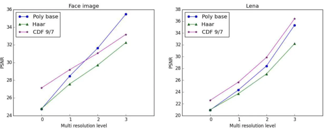
3.7 PSNR evolution using the brute force restrictions on coefficients for Lena and MUG face image . . . 35

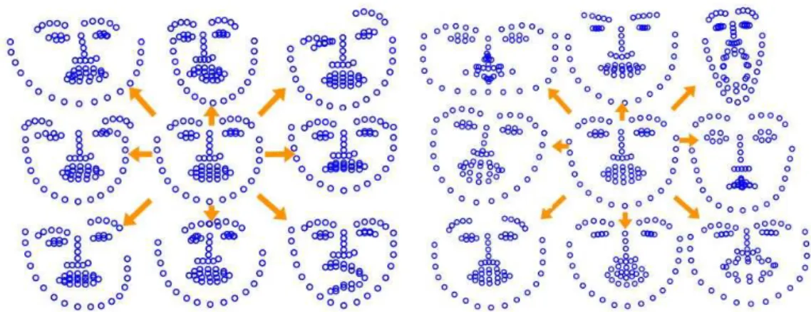
3.8 Reconstruction using 0 and 1 level coefficients after a 4 level decomposition. From left to right: complete basis, Haar an CDF 9/7 wavelets . . . 35

(16)

3.9 Reconstruction using 0-2 levels coefficients after a 4 level decomposition.

From left to right: complete basis, Haar an CDF 9/7 wavelets . . . 36

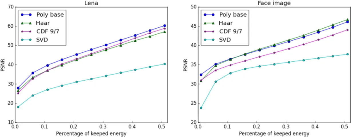
3.10 PSNR evolution using a fixed amount of energy coefficients for Lena and MUG face image . . . 36

3.11 Reconstruction using 1 percent of the coefficients. From left to right: SVD, complete basis, Haar an CDF 9/7 wavelets . . . 37

3.12 Reconstruction using 15 percents of the coefficients.From left to right: SVD, complete basis, Haar an CDF 9/7 wavelets . . . 37

4.1 Deformable model of shape in an AAM. Taken, from [MB04] . . . 40

4.2 Deformable model of appearance in an AAM. Taken, from [MB04] . . . . 41

4.3 Face matching example on IMM database . . . 45

4.4 Face matching example on MUG database . . . 46

4.5 Face matching example on Cohn Kanade database . . . 46

4.6 Face matching example on CMU MultiPie database . . . 47

4.7 Boxplots of alignment error vs compression ratio using Hermite 3 × 3 and Chebychev 10 × 10 bases. Wiskers are 1.5 IQR at maximum . . . 52

4.8 Real image . . . 52

4.9 Face synthesis using n percents of the coefficients.From left to right compres-sion ratio corresponding to : 40,30,20,15,10,5. On the first line the images are synthesised using Chebychev 3x3 basis and the second one Hermite 10x10 basis. . . 53

4.10 Cumulative errors on key points for the various datasets . . . 54

4.11 Boxplots of alignment error vs compression ratio using CDF 9/7 wavelets and Haar wavelets . Wiskers are 1.5 IQR at maximum . . . 55

4.12 Average alignment errors vs compresion ratio. Error bars are on standard error. . . 56

5.1 Images used for template alignement . . . 60

5.2 Images used for template alignement . . . 61

5.3 Cumulative errors on key points for the various datasets using the Newton (dotted line) and polynomial Newton (solid line) algorithms . . . 68

5.4 Comparison of the cumulative error on keypoints points on MUG database using different approaches . . . 70

6.1 Field of normals of a color image . . . 73

(17)

List of Figures xvii 6.3 Identical vector field parts computed at different scales : left -scale = 1 et

center - 4 and right 16 see restricted area in Figure6.2. . . 76

6.4 Vector fields computed at scale = 2 and resolution = 1 (left), scale =8 and resolution4 (center), and scale = 16 and resolution 8 (d) see restricted area in Figure6.2. . . 76

6.5 Extract of a normal vector field and its singular points detected using the next parameters :L = 1, D = 1, LS = 2, DS = 1, δΩ = 1, LV = 2, δ∗= 0. Red squares indicate the area in the selection of the singular point. . . 78

6.6 Up : SIFT keypoint detection (left), Box image (input image), SURF keypoint detection. Down : Singular keypoint detection, using C1 (left), C2 (center) and C3 (right) parameters . . . 79

6.7 Up : SIFT keypoint detection (left), Girl1 image (input image), SURF keypoint detection. Down : Singular keypoint detection, using C1 (left), C2 (center) and C3 (right) parameters . . . 80

6.8 Up : SIFT keypoint detection(left), Girl2 image (input image), SURF keypoint detection. Down : Singular keypoint detection, using C1(left), C2(center) and C3(right) parameters . . . 80

6.9 Pyramid representation using r (resolutions) and s (scales) . . . 81

6.10 Left - SIFT detector (223) and right- SURF detector(144) . . . 84

6.11 Polynomial sigularities detector sizes (left) and orientations (right) . . . 84

6.12 Left - SIFT detector (639) and right- SURF detector(1127) . . . 85

6.13 Polynomial sigularities detector (524) sizes (left) and orientations (right) . . 85

6.14 Example images used for the evaluation tests. Images (a) - (e) are from the Oxford dataset, Images (f)-(h) are from the additional dataset . . . 86

6.15 Averaged computation times for the different detectors . . . 89

6.16 Repeatability (up) and precision (down) under rotation transformations . . . 91

6.17 Repeatability (up) and precision (down) under blur transformations . . . 92

6.18 Repeatability (up) and precision (down) under brightness transformations . 93 6.19 Repeatability (up) and precision (down) under scale transformations . . . . 94

6.20 Repeatability (up) and precision (down) under illumination changes . . . . 95

6.21 JPEG compression repeatability (up) and precision scores(down) . . . 96

6.22 Repeatability (up) and precision (down) under zoom and rotation changes . 98 6.23 Repeatability (up) and precision (down) under zoom and rotation changes . 99 6.24 Detected areas in a face image . . . 100

(18)

7.2 Frequency decomposition of the polynomial transform, where hi, j represent

different subbands . . . 104

7.3 Gabor wavelets used for feature extraction . . . 105

7.4 On first row - original images, on second row, modified images using Global Procrustes normalization. Left : MUG , Right : Cohn-Kanade database . . 107

7.5 Comparison of proposed approaches with other methods in terms of classifi-cation accuracy using annotated points . . . 109

7.6 Comparison of proposed approaches with other methods in terms of classifi-cation accuracy using normalized annotated points . . . 109

7.7 Comparison of proposed approaches with other methods in terms of classifi-cation accuracy using calculated points . . . 111

7.8 Comparison of proposed approaches with other methods in terms of classifi-cation accuracy using normalized calculated points . . . 111

(19)

List of Tables

3.1 Some weighting functions w to obtain different families of polynomials . . 27

4.1 Mean Error pixel/landmark . . . 45

4.2 Mean error on face interior points . . . 53

4.3 Mean ± standard deviation using RAW DAAM and CDAAM methods . . 53

5.1 Polynomial coefficients for a 3 × 3 Legendre basis . . . 59

5.2 Comparative results for face template matching. . . 60

5.3 Comparative results for face template matching. . . 62

5.4 Mean ± standard deviation using ICIA and Polynomial ICIA methods . . . 65

5.5 Mean error on face interior points . . . 65

5.6 Mean ± standard deviation using Newton and Polynomial Newton methods 67 5.7 Mean error on face interior points . . . 67

6.1 Mean repeatability scores for Bark and Boat sequences . . . 98

6.2 Experimental results on MUG database . . . 100

6.3 Experimental results on IMM, Cohn-Kanade and MultiPie databases. . . 101

7.1 Confusion matrix for the CK database (SR_Poly) . . . 106

7.2 Confusion matrix for the MUG database (SR_Poly) . . . 107

7.3 Confusion matrix for the CK database (SR_Poly) using normalized images 108 7.4 Confusion matrix for the MUG database (SR_Poly) using normalized images108 7.5 Comparison of proposed approaches with other methods in terms of execu-tion times. . . 110

(20)

Acronyms / Abbreviations

AAM Active Appearance Models

CDAAM Compressed Discriminative AAM CLM Constrained Local Models

CPR Cascaded Pose Regression

FT-PAAM AAM retrieved from a multi-resolution polynomial decomposition of the full aligned texture

PAAM AAM calculated using polynomial projections on texture patches sampled around key landmarks

PDM Point Distribution Model SVM Support Vector Machine

(21)

Chapter 1 Introduction

The face is a very rich source of information on non-verbal communication. Although a human observer is able to perceive naturally some of this information from visual observa-tions, its analysis remains a very difficult task in computer vision. As one of the most active and visible research topics in pattern recognition, biometrics and image processing, facial analysis has been extensively studied in the past two decades due to its many application areas such as security (surveillance, biometrics), human-machine interaction, robotics, indexation, behavior analysis etc.

Face analysis research includes several themes : detection, tracking, localization, recog-nition, authentication, face synthesis. Algorithms used for face analysis face multiple challenges, including both intrinsic (pose or facial expression of the subject) and extrinsic pa-rameters, such as partial occlusions or conditions of image acquisition (luminance problems, shadows).

During the course of this thesis, we will be mainly interested in polynomial modeling applied to face analysis and more specifically to deformable models : a set of methods that provide the abstract model or approximation of an object class. They model separately the variability in shape, texture or imaging conditions of the objects in the class (e.g. human faces), using a defined number of parameters. Polynomial representations have simple expression, allow to describe discrete sets of values (ie image pixels) by analytical functions and fit geometrical forms of images harmoniously. Slowly varying surfaces (like facial skin) in images are well represented by polynomials and their reconstruction quality is pleasant to the human eye.

The work presented here will primarily investigate the usage of polynomial representation applied to multiple face analysis steps, from face texture modeling and compression or facial keypoints detection to descriptors for facial expressions classification.

(22)

1.1 Motivation

The work presented in this thesis was motivated by a practical application for facial animation, and more generally the synthesis of human characters and scenes for the entertainment industry (video games, animated films).

This is usually done through automation or semi-automation of a part of the synthesis process based on a complex analysis of facial expressions and head movements. Traditionally, such animations are entirely produced by skilled actors on which are positioned markers. Although this type of animation gives the best quality results, its associated implementation process is slow and expensive because it requires a specific makeup and usually involves multiple cameras. Moreover, it is particularly inconvenient for the actors and for later video captures. Recent advances in image processing make possible the detection of facial features that can be exploited for automatic animation, without the use of markers. They provide animated meshes that can be injected into the synthesis and animation software, both in post-production and live, thus allowing to save time and providing significant shooting facilities.

Yet it is still a challenging problem in practice due to uncontrolled environment, occlu-sions and variations in pose, illumination, etc. Various methods have been proposed for facial features extraction, with different advantages and drawbacks in terms of robustness, computational cost and accuracy. Recent advances in image representation show that most low-level descriptors used in said methods rely on ill-defined frameworks.

A good example of low-level image descriptor is the Gabor space. Neurophysiological studies show evidence that the human visual system (HVS) is best modeled as a family of self-similar 2D Gabor functions [Dau85]. Like the Haar transform, the Gabor transform is considered as the mother wavelet in time-frequency analysis theory and is often used in facial analysis-related computer vision applications to create sparse object representations.

Despite their high accuracy, the use of Gabor filters in image processing is often criticized in terms of computational cost. Therefore we decided to study the case of another image representation having similar properties to the HVS, namely the orthogonal polynomials [Bla74]. Within the framework suggested by Blaivas, visual analysis in the retina can be regarded as a process of expansion in orthogonal polynomials basis. Motivated by this property, and by the results obtained concerning the use of orthogonal polynomials for human motion analysis in [KTAK10] we propose to use the coefficients derived from polynomial projection in several face analysis applications.

Therefore we will use bivariate orthogonal polynomials to construct 2D wavelet func-tions and to define a multiresolution wavelet-like image transform. We will see later that with respect to classic time-frequency representations, such as wavelets, polynomial basis

(23)

1.2 Thesis outline 3 decompositions do not necessarily use a dyadic partition and are therefore more adaptable. The polynomial multi-resolution decomposition will allow to organize hierarchically the image information within the frequency domain. As a result, polynomial coefficients can be used as an efficient alternative to global or redundant texture representations such as Gabor Wavelets, without losing accuracy.

The purpose of the thesis is to study 2D polynomial modeling for image representations and see their impact in facial analysis applications (pose/landmark/expression detection for avatar animation, emotion detection, facial keypoints) in terms of robustness, accuracy and computational cost.

1.2 Thesis outline

This document is organized into three parts.

First, in chapter2 a review of state of the art in face landmarking is presented. This review includes work on parametric and non parametric models for facial landmarks localiza-tion. This chapter is important to understand the motivation behind the work in this thesis. Chapter3begins with the presentation of a method to generate orthogonal polynomials bases. Follows the 2D polynomial image approximation that allow to obtain a null approximation error and the construction of a multiresolution piecewise polynomial decomposition. The chapter ends with the presentation of the strategies for polynomial coefficient selection in the approximation process.

Chapter4and5are dedicated to the integration of polynomial bases in deformable models and mainly the Active Appearance Models (AAM) algorithm. In chapter 4 we explore the way polynomial coefficients can be used for texture analysis and representation. First we detail the AAM framework and propose two different schemes to replace the original AAM texture representation model by approximating image structures with polynomial projections on an orthonormal basis. Next we extend an existing work applied to face alignment where wavelet coefficient subsets were modeled rather than pixel intensities by using subsets of polynomial coefficients. Deviating from the existing approach the approximation coefficients are included in a regression framework. In chapter5we will take an interest in the generative fitting, review in details the inverse compositional approach and see how the polynomials can be used to replace analytically the computation of gradients in the Gauss Newton and Newton descent gradient approach using projections on the first and second order basis polynomials.

(24)

The last part of this thesis have concentrated on the use of polynomial bases for keypoint detection and for facial expression recognition. Chapter6begins with the definition of the detection algorithm. First we show how to compute an image vector field of normals and then we present the selection of interesting points in a multi-scale and multi-resolution scheme. We evaluate next and compare to nine recent detectors our method on the Oxford dataset. We detail then how areas detected with our algorithm can be used in the AAM for a sparse texture model. Finally, in Chapter7we detail the way in which the results of the tracking algorithm can be exploited to the description of expressions. We first present a polynomial based texture representation model as a descriptor for facial expression information. We introduce two different modes for the descriptor calculation and compare in terms of computational efficiency the polynomial and Gabor transforms. We finish by describing the experimental results on two different databases.

1.3 Main contributions

The contributions of this thesis are consistent with the logical flow of the chapters. The first contributions rely to the discriminative fitting approach. We propose a new approach for texture representation in deformable models, and the inclusion of the polynomial coefficients in a regression framework to have a compressed polynomial texture model. The second contributions rely with the generative fitting approach. We propose to adapt the inverse compositional approach using polynomial bases both for the gradient descent algorithm as for the texture representation model. Finally, we investigate the use of polynomial bases for interesting points detection and facial expressions classification.

A more detailed description of the contributions is presented here:

• Since model fitting parameters are estimated by minimizing the sum of squared dif-ferences of texture values between observations and approximations, accuracy and robustness will rely heavily on choices regarding texture representation. In the polyno-mial texture representation for deformable models we use coefficients resulting from polynomial projections of pixel values for image approximation. By comparing our approach to PCA-based global analysis of raw pixel intensities one can usually find in AAM texture models we demonstrate it’s ability to improve robustness against pose and facial expression changes.

• The state of the art AAM texture models explicitly model the value of every pixel covering an object. To avoid the excessive computational requirements for high

(25)

1.3 Main contributions 5 resolution images we propose to use a compressed polynomial texture model. This work is an extension of the work of Wolstenholme and Stegmann [SFC04] where Haar and CDF 9/7 wavelet coefficient subsets were modeled rather than pixel intensities. We demonstrate the straightforward integration of compressed polynomial coefficients in the texture model of an AAM and introduce a framework that incorporates polynomial compression into a cascaded regression.

• Considering the polynomial approximation equivalent to a filter bank, we show first how the polynomial coefficients can be used in a gradients descent algorithm. Next we reformulate the inverse compositional algorithm to entertain fitting across multiple polynomial filter responses and show how using polynomial bases in the Gauss Newton and Newton gradient descent algorithm limits the computation error and induces better alignment results.

• We describe an algorithm for points of interest detection that works not only on grayscale images (as the majority of recent detectors) but also on color images. This algorithm offers the possibility to use different types of bases (and therefore use different types of smoothing in the construction of scale pyramids) while creating the multivariate basis and allows to select the number of detected features using simple thresholds. The facial regions chosen by our algorithm are also included in an AAM texture model.

• Finally we propose to use polynomial bases for feature extraction within a system of facial expression recognition. Two different modes for the description are presented, using the single or multi resolution approach polynomial projections. In the single resolution approach the coefficients provide a hierarchical representation of image structures, therefore their number is reduced to speed-up the computations with little efficiency loss. The multi resolution approach is showed to be more compact than a Gabor wavelet representation, thus allowing the disappearance of most sampling problems, such as the trade-off between orientation sampling and spatial sampling. • The performance of all the proposed method and algorithms is evaluated and compared

(26)

(27)

Chapter 2 Recent advances in face landmarking

2.1 Introduction

A landmark represents a distinguishable point present in most of the images under consid-eration, for example, the location of the left eye pupil. Facial landmark estimation seeks to automatically locate predefined facial landmarks in face images (Fig. 2.1). It is an important research area in computer vision in part because digital face portraits are ubiqui-tous. Accurately modeling human faces is key for a number of visual tasks such as facial recognition [ND09, WFKVDM97], face reconstruction [KSS11], expression recognition [Bet12,LMH+₀₆_{], facial animation [}_CWLZ13_{] or biomedical applications [}_BML+₀₁_{] to}

name just a few.

Figure 2.1 A face with correctly positioned landmarks

Robust facial landmark estimation is very challenging in practice, due to a variety of factors such as acquisition cameras, physiognomies, illumination effects, occlusions or poses.

(28)

Furthermore accurate and precise landmarking remains a difficult problem since, except for a few, the landmarks do not necessarily correspond to high-gradient or other salient points. Hence, low-level image processing tools remain inadequate to detect them, and recourse has to be made to higher order face shape information.

Early work on the facial landmark localization [EFM09] often addressed the problem as a particular case of the object part detection problem. However, general detection methods are not adapted to detect facial landmarks because as mentioned before few salient markings (eg, centers for eyes, lips) can be characterized reliably by their image appearances. Therefore, shape constraints or support neighboring areas are essential for augmenting weak local detectors. According to the type of constraints imposed previous work can be classified into two groups: the parametric methods and non parametric methods.

The majority of methods described lower depends on a good face initialization. A popular strategy, even for recent approaches (e.g., [AZCP13], [CWWS14], [CCTC09], [XDlT13] to name just a few), is to first detect the face (i.e., using [VJ04]), and then fit a mean face shape (where the shape is defined by the facial landmarks) to the detection window. However, for extreme poses and some expressions, traditional face detectors (e.g., [VJ04]) may fail, or the true shape of the face inside the detection window will differ significantly from the initial shape, making a good initialization unlikely.

Part-based models [FGMR10], [YR11] can be used to address the initialization problem, but learning an accurate part graph parameterization and inferring part labels from the graph can be challenging. Recent works [YHZ+₁₃_{], [}_ZR12_{] simplify the graph structure to a tree}

and produce impressive results.

Though it is possible to build separate Active Appearance Models or Active Shape Models to handle pose variation (view-based models), as carried out in [CWWT02], [RGP+₉₉_]

[ZA06] and [MBN13], respectively, the fact that they require very accurate initialization decreases their effectiveness, especially on real-world images, where the simultaneous effects of pose (yaw, pitch, and roll) and facial occlusions can decrease their accuracy. Thus, there has been a recent increase in literature dealing with the automatic landmarking of non-frontal faces using various unique approaches. Everingham et al. [ESZ06] used a generative model of facial feature positions (modeled jointly using a mixture of Gaussian trees) and a discriminative model of feature appearance (modeled using a variant of AdaBoost and "Haar-like" image features [VJ01]) to localize a set of 9 facial landmarks.

(29)

2.2 Parametric models 9

2.2 Parametric models

Traditionally facial landmarking has been carried using deformable template (parametric) based models that can roughly be divided into two main categories: (a) Holistic Models that use the holistic texture-based facial representations; and (b) Part Based Models that use the local image patches around the landmark points. Notable examples of the first category are Active Appearance Models (AAMs) [CET01a],[TAiMZP13] and 3D deformable models [BV03]. The second category includes models such as Active Shape Models (ASMs) [CTCG95], Constrained Local Models (CLM) [SLC11] and the tree-based pictorial structures [ZR12]. We will not discuss here the 3D deformable models.

2.2.1 Active Shape Models

The Active Shape Model (ASM) was introduced by Cootes et al. [CTCG95] as a method of fitting a set of local feature detectors to an object and simultaneously taking into account global shape considerations. The allowable shape deformations are learnt from a manually labelled training set to produce a linear shape model with the following form:

s = ¯s + Psbs (2.1)

where ¯s is the mean shape, Ps is a set of orthogonal modes of variation and bs is a set

of shape parameters. An illustration of a statistical distribution of facial feature points is represented in Figure2.2. There are 600 shapes (smaller dot points in black) normalized by Procrustes analysis. The larger dot points in red indicate the mean shape of all shapes.

Various shapes can be generated with Equation2.2by varying the vector parameter bs.

By keeping the elements of bswithin limits (determined during model building) the generated

face shapes are lifelike. Conversely, given a new shape ˜s, the parameter b that allows to produce ˜s given a model shape ¯s can be calculated.

Cootes and Taylor [CT+₀₄_{] describe an iterative algorithm that gives the b}

sand T that

minimizes

distance(˜s, T(¯s + Psbs)) (2.2)

where T is a similarity transform that maps the model space into the image space.

Many modifications to the classical ASM have been proposed over the years, such as in [MN08], [SS09], that have mainly focused on developing better local texture models, however they still remain susceptible to occlusions, the problem of local-minima, and are very dependent on good initialization Other improvements focus on the local detectors. For

(30)

Figure 2.2 Statistical distribution of facial feature points. Figure taken from [WGTL14] example, Boosted Regression Active Shape Models [CC07] use boosting to predict a new location for each point, given the patch around the current position.

Among the methods focusing on a more robust global shape prior, Everingham et al. [ESZ06] model the face configuration using pictorial structures [FH05], a hierarchical version of which was used in [RBDlT+₁₁_{]. Valstar et al. [}_VMBP10_{] combine SVM regression for}

estimating the feature point’s location with conditional Markov random fields to keep the estimates globally consistent. They also take advantage of facial feature points whose position is less sensitive to facial expressions; they thus start by localizing such stable points first and then find the additional points after a registration step. The whole process takes around 50 seconds per image. Very recently, Amberg and Vetter [AV11] proposed to run detectors over the whole image and then find the optimal set of detections using Branch & Bound; however, they only show results for high-quality images and need over one second to process one image.

ASMs belong to a class of methods that can be broadly referred to as Constrained Local Models (CLMs) [CC06], [CC08], [SLC11] (see2.2.3).

2.2.2 Active Appearance Models

An AAM is a statistical model introduced by Cootes et al [CET01a] which describes shape and texture variabilities of an object learned from a training set comprising different views of the object.

Similar to ASMs, active appearance models are created from manually annotated data with key landmarks points images and where the variations between the positions of points -the shape x and -the pattern of intensities or colors across an image patch - -the texture g, are learned by principal component analysis. Any example can be approximated using :

(31)

2.2 Parametric models 11 s = ¯s + Psbs a = ¯a + Paba (2.3)

where ¯s and ¯a are respectively the mean shape and texture, Ps, Paare matrices describing

the modes of variation derived from the training set. A third PCA is then performed on a concatenated shape and texture parameters b, to obtain a combined model vector c:

b = Qc (2.4)

From the combined appearance model vector c, a new instance of shape and texture can be generated:

smodel= ¯s + PsWsQsc amodel= ¯a + PaQac (2.5)

where Wsis a diagonal matrix of weights for each shape parameters and

Q = ( Qs Qa ) (2.6) Fig. 2.3shows the effect of varying the first four parameters from c, showing changes in identity, pose, and expression. Note the correlation between shape and intensity variation.

The goal of the active appearance model is to find the appearance parameters giving the best match to an unseen image. Both ASMs and AAMs build shape models (also referred

Figure 2.3 Effect of varying first four facial appearance model parameters, c1− c4 by ±3

standard deviations from the mean. Taken from [CET01a].

to as Point Distribution Models (PDMs)), that model the shape of a typical face that is represented by a set of constituent landmarks, and texture models of what the region enclosed by these landmarks looks like. The difference between the two is that ASMs build local texture models of what small 1D or 2D regions around each of landmarks look like, while AAMs build global texture models of the entire convex hull bounded by the landmarks.

(32)

The two main assumptions behind AAMs are that (1) for every test (unseen) image there exists a test shape and set of texture weights for which the test shape can be warped onto the reference frame and expressed as a linear combination of the shape-free training textures and (2) the test shape can be written as a linear combination of the training shapes.

Defining a linear statistical model of texture that explains variations in identity, expres-sions, pose and illumination, is a very challenging task, especially in the intensity domain. Furthermore, the large variation in facial appearance makes it very difficult to perform regression from texture differences to shape parameters. That’s why numerous extensions of standard AAMs have been proposed to improve their fitting quality.

The majority of AAM extensions can loosely be categorized based on how they tackle the problem, with the most common strategies being: (1) improvement of the actual fitting procedure by changing the factors involved in the optimization (e.g. [GMB05], [CT06], [MB04],[GMB06]); and (2) usage of more robust feature representations, e.g. to obtain invariance with respect to occlusions [TAiMZP13], illumination [NSL11], or non-linear shape deformations [HM09].

One of the main disadvantages of the algorithm, as for instance stated in [TAiMZP13], [GMB05], [CT06],[Liu10], [PPB08], [SK09] is their weak generalization ability when learned with only a few training examples that do not cover the complete range of possible variations in the data. To overcome this problem Zhao et al. [ZSCC13] proposed computing a separate AAM for each test face using k-nearest neighbor training faces (w.r.t. the test face) rather than all training faces. Using k-NN exemplars is an important part of the approach of [BJKK11] [ZBL13],[SLBW13].

To align unknown faces in unknown poses and illuminations, [SLGBG09] proposed to use specific transformation of the active model texture in an oriented map, which changes the AAM normalization process and to do the research in a set of different precomputed models related to the most adapted AAM for an unknown face.

The classic AAM approach is computationally expensive and sensitive to the initializa-tion due to the involved gradient descent based optimizainitializa-tion[YHL+₀₃_,_CILS12_,_XDlT13_,

CWWS14].

Recently, Tzimiropoulos and Pantic [TP13] proposed new optimizations for fast and accurate AAM fitting and demonstrated better fitting results on unseen images with a large range of pose variation using a more unconstrained training set drawn from the Labeled Face Parts in the Wild (LFPW) dataset [BJKK11].

Approaches which increase the expressiveness of an AAM are very rare. One example is the Online Appearance Model [SK09], where the texture component is constantly being updated via incremental PCA during model fitting to account for illumination changes.

(33)

2.2 Parametric models 13 Similarly, Adaptive AAMs [Liu10] feature a generic and a subject-specific texture component, where the latter is again being updated during fitting. However, both methods add knowledge to the model only at fitting time and, both approaches update only the texture component, which, for instance, excludes the possibility to add new facial expressions to existing AAMs. Although the well known inverse compositional ICIA algorithm [MB04] has been crit-icized for its inability to perform well under generic fitting scenarios, i.e. to fit images of unseen identities, the algorithm is very popular, mainly because of its extremely low computational complexity, and methodologies such as [PM08][ABV09], which can provide near real-time fitting, has not received much attention. It has been demonstrated that ASMs are more suited to the task of precise facial landmarking than AAMs [CET01a], [SS12], [CWWT02], [CT+₀₄_{], [}_BM04_{] [}_CET99_{], as AAMs are generative, global texture based}

approaches and are more easily affected by variations in illumination and the presence of occlusions.

Compared to ASMs, AAMs generalize poorly to unseen faces, however for tasks where generalizing across people is not necessary and one has access to several training images of an individual, AAMs work very well and are able to learn a holistic representation of the face. Therefore active appearance models, are useful for many tasks like face inpainting, detecting and removing occlusion, face identification, face animation.

2.2.3 Part based models

The part based models [ZR12] ,[CC08], [SLC11], [BJKK11], [CILS12] perform face align-ment by maximizing a posterior probability of part locations given the image and then fuse the probabilities of all the parts together enforced by a global shape model, e.g. enhanced ASM [CC08], [SLC11] or pictorial structures [ZR12], to generate the final result.

The main advantages of part-based models [SLC11],[ZR12], [AZCP13] (i.e. models which do not define a complete holistic texture model of the object) are a natural handling of partial occlusions (since they only model certain parts of the object) and, most importantly, the fact that they are optimized only with respect to shape (they do not define parametric models of texture). Notable examples include Constrained Local Models (CLMs) [SLC11] and the tree-based model of [ZR12] (which can be also used for object detection). More recently, Asthana et al. [AZCP13] proposed a robust discriminative framework for fitting CLMs which achieved state-of-the-art results in the problem of facial alignment "in the wild".

(34)

CLM

CLMs [CC08], build local models of texture variation around landmarks (sometimes referred to as "patch experts" and allow landmarks to drift into the locations that best match training data using these patch experts. This is similar to the AAM; however, the texture sampling method is different. The shape is then regularized using the shape model to generate a plausible set of final landmark locations. Unlike AAM which tries to approximate the raw image pixels directly, the constrained local models [CC08] employ an extended appearance model to generate the feature templates of the parts, which obtains improved robustness and accuracy. The search algorithm is presented in Fig.2.4.

Figure 2.4 Constrained Local Model (CLM) search algorithm. Taken from [CC08] The local appearance models are more robust to a range of challenges including occlu-sion and global illumination changes, but CLMs still rely on parametric shape models for regularization, which may not generalize well to a broad range of poses.

Saragih et al. [SLC11] proposed to use linear SVMs over power normalized image patches to discriminate aligned from misaligned mesh vertex coordinates. Composing the SVM classification score with a sigmoid function generates a likelihood map over the vertices within a local search region around its current estimate. This allows a Bayesian treatment of the alignment problem. Asthana et al. [AZCP13] developed a discriminative regression based approach for the CLM framework that they referred to as Discriminative Response Map Fitting (DRMF). DRMF represents the response maps around landmarks using a small set of parameters and uses regression techniques to learn functions to obtain shape parameter updates from response maps.

(35)

2.2 Parametric models 15 Tree based models

In their recent seminal work, Zhu and Ramanan [ZR12] proposed an elegant framework that built on the previously developed idea of using mixtures of Deformable Part Models (DPMs) for object detection [FGMR10] to simultaneously detect faces, localize a dense set of landmarks, and provide a course estimate of facial pose (yaw) in challenging images. Their approach used a mixture of trees with a shared pool of parts V to model each facial landmark. Global mixtures were used to capture changes in facial shapes across pose and the tree-structured models were optimized quickly and effectively using dynamic programming. The approach is quite effective at handling a wide range of yaw variation but does not account for excessive in-plane rotation of faces or large occlusion levels.

In their tree structured part model each tree is written Tm= (Vm, Em) as a

linearly-parameterized, tree-structured pictorial structure, where m indicates a mixture and Vm⊆ V .

Taking an image I , and the pixel location of part i as li= (xi, yi) a configuration of parts

L_{= {l}i: i ∈ V} is scored as:

S(I, L, m) = Appm(I, L) + Shapem(L) + αm (2.7)

Appm(I, L) =

∑

i∈Vm wm_i _{· φ(I,l}i) (2.8) Shapem(L) =

∑

i j∈Em am_{i j}dx2+ bm_{i j}dx+ cm_{i j}dy2+ d_{i j}mdy (2.9) Equation 2.8 sums the appearance evidence for placing a template wm

i for part i, tuned

for mixture m, at location li . φ (I,li) represent the feature vector (e.g., HoG descriptor)

extracted from pixel location liin image I. Equation.2.9scores the mixture-specific spatial

arrangement of parts L, where dx = xi− xj and dy= yi− yj are the displacement of the

ith part relative to the jth part. Each term in the sum can be interpreted as a spring that introduces spatial constraints between a pair of parts, where the parameters (a,b,c,d) specify the rest location and rigidity of each spring. Finally, the last term αm _{is a scalar bias or}

"prior" associated with viewpoint mixture m.

A comparison of the learned shape models with those trained generatively with maximum likelihood is presented in Fig. 2.5. Tree based SVM captures much of the relevant elastic deformation, but produces some unnatural deformations because it lacks loopy spatial constraints.

Since pose is part of estimation, the algorithm practically works as a multiview algorithm. In contrast to [VMBP10], [MVBP13] where local and global information are invoked in succession, this algorithm is shape driven, and local and global information are merged

(36)

right from beginning. This is implemented by considering several (30 to 60) local patches that are connected as a tree, which collectively describe the landmark related region of the face; in other words, the patch-based face graph models the ROI of the detected face and incorporates its pose and landmark information. This approach is an adaptation of the idea of tree-structured pictorial structures [FGMR10].

Recently, Ghiasi and Fowlkes [GF14] built on this work and proposed a hierarchical deformable part model for face detection and landmark localization to explicitly model the occlusion of parts and hence achieved more accurate results on challenging occluded images in the wild.

Tree-structured pictorial structures have also been successfully applied to face recognition by Everingham et al. [CWWS14], where the local appearance of each landmark is learned by a variation of Adaboost algorithm with Haar-like features [VJ04]. Similarly, Uricar et al. [UFH12], inspired by pictorial structures, jointly optimize appearance similarity and deformation cost with a parameterized scoring function where the parameters are learned from manually annotated instances using the structured output SVM classifier.

Figure 2.5 Mean shape and deformable models for tree based SVM (left) and AAM (right). Taken from [ZR12]

2.3 Non parametric models

Despite the success of parametric shape models, the model flexibility (e.g., PCA dimension) is often heuristically determined. Furthermore, using a fixed shape model in an iterative alignment process (as most methods do) may also be suboptimal. This is the reason, recently non parametric methods have emerged.

(37)

2.3 Non parametric models 17

2.3.1 Shape regression

Recently, a variety of approaches [CWWS14],[BAPD13],[YLYL13], [KJ14] that can be broadly grouped under the category of shape regression based approaches have emerged. Regression based methods can achieve accurate results at great speed and have thus become quite popular. All these methods are improved variants of the original approach called Cascaded Pose Regression (CPR) and introduced by Dollar et al. [DWP10].

CPR is formed by a cascade of T regressors R1..T that start from a raw initial shape guess S0 and progressively refine estimation, outputting final shape estimation ST . Shape S is represented as a series of P part locations Sp= [xp; yp], p ∈ 1..P . At each iteration, regressors

Rt produce an update ∂ S, which is then combined with previous iteration’s estimate St−1to form a new shape.

The training procedure for a CPR is shown in Alg. 1. During learning , each regressor Rt is trained to attempt to minimize the difference between the true shape and the shape estimate of the previous iteration St−1_{using landmark-indexed features h}

t. For simplicity, we

use the notion of "landmark-indexed" feature instead of "pose indexed features" used by the authors of [DWP10]. S0is the single pose estimate that gives the lowest training error without

relying on any component regressors. The available features depend on the current shape estimate and therefore change in every iteration of the algorithm; such features are known as landmark-indexed features. The key to CPR lies on computing robust landmark-indexed features and training regressors able to progressively reduce the estimation error at each iteration.

Algorithm 1 Training for cascaded Pose Regression (taken from [DWP10]) Input: Data (Ii, Si) for i = 1..N

1: S0= arg minS∑id(S, Si) 2: S0_i = S0for i = 1...N 3: for t = 1 to T do 4: xi= ht(St−1, Ii) 5: ˜S = ¯St_i−1_{◦ S}i 6: Rt= arg minR∑id(R(xi), ˜Si) 7: St_i= St_i−1_{◦ R}t_(x i) 8: εt= ∑id(Sti, Si)/ ∑id(Sti−1, Si) 9: If εt ≥ 1 stop 10: end for 11: Output R = (R1, ..., RT₎

After the training step, given an input shape S0, the regressor R(S0; I) is evaluated by

computing: St _{= S}t−1_{◦ S}