Boundary element analysis of an integral equation for three-dmensional crack problems

HAL Id: hal-01005293

https://hal.archives-ouvertes.fr/hal-01005293 Submitted on 28 Oct 2016

HAL is a multi-disciplinary open access archive for the deposit and dissemination of sci-entific research documents, whether they are pub-lished or not. The documents may come from teaching and research institutions in France or abroad, or from public or private research centers.

L’archive ouverte pluridisciplinaire HAL, est destinée au dépôt et à la diffusion de documents scientifiques de niveau recherche, publiés ou non, émanant des établissements d’enseignement et de recherche français ou étrangers, des laboratoires publics ou privés.

Distributed under a Creative Commons Attribution| 4.0 International License

Boundary element analysis of an integral equation for

three-dmensional crack problems

Anh Le Van, Bernard Peseux

To cite this version:

Anh Le Van, Bernard Peseux. Boundary element analysis of an integral equation for three-dmensional crack problems. International Journal for Numerical Methods in Engineering, Wiley, 1988, 26 (11), pp.2383 - 2402. �10.1002/nme.1620261104�. �hal-01005293�

BOUNDARY ELEMENT ANALYSIS OF AN INTEGRAL

EQUATION FOR THREE-DMENSIONAL CRACK

PROBLEMS

A. LE V AN• AND B. PESEUX'

Laboratoire de Mecanique des Structures, Ecole Na1tionale Superieure de Mecanique, /, ra4re de Ia Noe, Nantes 44072 Cedex, France

SUMMARY

In another paper, the authors proposed an integral equation for arbitrary shaped three-dimensional cracks. In the present paper, a discretization of this equation using a tensor formalism is formulated. This approach has the advantage of providing the displacement discontinuity vector in the local basis which varies as a function of the point of the crack surface. This also facilitates the computation of the stress intensity factors along the crack edge. Numerical examples reported for a circular crack and a semi-elliptical surface crack in a cylindrical bar show that one can obtain good resuhs, using few Gaussian poilnts and no singular elements.

INTRODUCTION

The integral equation method has been thoroughly experienced in structure analysis. Integral equations derived from the Somigliana representation were successfully applied to three-dimensional problems, such as in References 1 and 2. In the latter reference, a particular symmetrical problem of cracked bodies was also investigated. Integral equations with kernels containing singular solutions, usually referred to as Kupradze elastic potentials, 3 are particularly well suited to crack analysis. The use of these potentials in linear fracture mechanics is advantageous as it permits one to obtain directly stress intensity factors from the computed vector density. Embedded cracks in an infinite medium were studied in References 4-7. In particular, Bui4 showed that for plane cracks the mode I is entirely uncoupled from modes II and III. Later on, integral equations for three-dimensional cracks were proposed;8• 9 in the last reference use was made of a Kupradze double layer potential, and the unknown was the vector density directly related to the displacement discontinuity through the crack surface. In this paper, we carry out the discretization of the integral equation proposed in Reference 9, with a view to studying imbedded or surface crack problems.

For numerical purposes, the main difficulty is the reckoning of singular integrals defined in the sense of the principal value. Cruse1 succeeded in giving the closed form of the principal value integral, using planar boundary elements. A more general way to evaluate two-dimensional singular integrals was investigated by K.azantzakis and Theocaris, 10 who also reduced these to one-dimensional finite-part integrals.11 Among the most recent works, one can find References 12 and 13 where exact expressions for some specific two-dimensional finite!-part integrals are derived.

As for Kupradze potentials, Bui4 took a small polygon instead of a circle to perform principal value integrals, it seems, however, that this procedure cannot be used with ease. Lastly, one can find in Reference 14 an improvement of the evaluatjon of integrals of order 1

/r,

1

fr

2, 1

fr

3, by means

of a minimum number of Gaussian points. As the considered distance

r,

small though it may be, remains always finite, these integrals are actually not singular ones. In any case, difficulties must certainly be expected when dealing with principal value integrals defined on curved surfaces.

In our analysis, we limit consideration to classical Gaussian quadrature, with no actual principal value computations. Nevertheless, two numerical examples given in the last section show that one can obtain fair results, using few Gaussian points, no singular integral computations and in particular, no singular elements around the crack edge. First, we deal with the embedded penny-shaped crack. The numerical results obtained proved to fit well to the analytical solution of Sneddon.15 Then we treat the problem of a semi-elliptical crack in a cylindrical bar under combined loads. In the opening mode, the numerical results can be compared to the existing results16- 18 which involved analogous crack geometries.

THEORETICAL BACKGROUND

Let us consider the problem of an elastic solid ~ containing an arbitrary shaped, imbedded or surface crack S, with the mixed boundary conditions:

y₀eSuD.: lim t(x, Dx)

=

tg(y0, Dyo)

!i)\S ~ x-. y~, n .. = n70

(Ia)

or: y₀eSuD: lim u(x) = u8_{(Yo) (lb)}

!i)\S3x-+y~

where the superscript g stands for given, and the double sign

+

is related to the surface orientation, locally defined by the normal nyo at each point y0 .

1. Displacement field expression

Let the displacement field be expressed by means of the Kupradze double-layer potential of the first kind3

u(x)= LTT(y-x, n,)<p(y)d,S (2)

where the density cp is a vector function defined in the crack S, and T the Kupradze tensor

2p, 6(1

+

p,)e,-ny

T(y- X, Dy) 8n(A.+ 2Jl)·r2 [ny®er-er®ny-(e,:ny)I]-8n(A.+ 2p,)·r2 er®er

1 is the unit tensor, r=

ll

y-x

!l

, e,.=(y-

x

)

/ll

y-x

l

!.

The displacement discontinuity on the crack is obtained from

[u(y_0)] =u(yri)-u(yi))='P<yo) (3)

Using (3), one can calculate the stress intensity factors which are now directly related to the density cp.

2. Integral equations

It was shown in Reference 9 that, under the assumptions SeC1_{·cz, O<a~ 1, <peCl.lf(S), 0<{3~ l,} the integral equation for a general crack is expressed by

Vy0ES, t(y 0 ,

O,.ol

=

16

7<(~

_

v

2 ) pv

1

(2(<1>. ••

e,

F. ,)n,0 - (1- 2

v)H+ .•• e,

n,.o) F., +(F,v·ny0)<P,u A e,)+3(e,-<P,u)((F,v, ny0 , e,)e,+(n10·e,)e, A F,v)

- 2(cl»,v, e,, F,u)Dyo

+

(1- 2 v )( (clJ,v, e,, Dyo) F,u

+

(F,u ·nyo)cl»,v A e,) - 3(e, ·<P,v)((F,u, Dy0 , e,)e,+(ny0 ·e,)e, 1\ F,u)) dudv

-16n(~-v2)

f ..

'C(n,o, y- Yo•

~)op(y)d,l

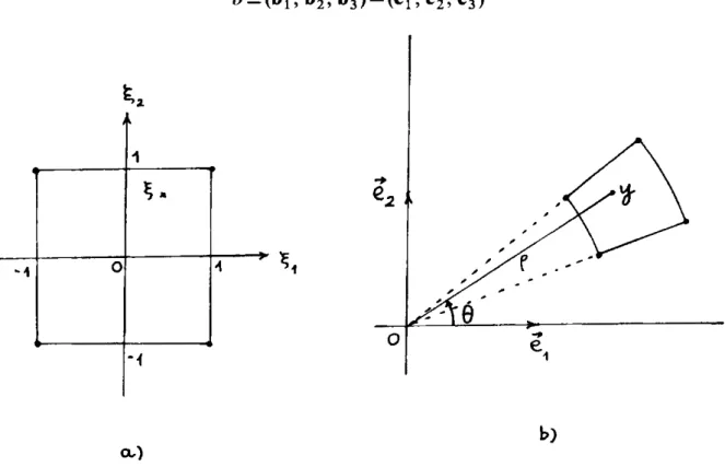
(4)

with now (Figure l): r=lly-y₀ ll,e,=(y-yo)/IIY-Yoll

F: a parametrization of S, defined on a domain A in IR2: A3(u, v)~ y

=F(u, v)ES

cJ»(u, v)=q>(F(u, v))=<p(y)

t: the unit vector tangent to the crack edge aS, oriented according to the orientation of S.

One should notice that the symbol pv before the two-dimensional integral relates to the principal value on S (not on A), and that the expression still holds in the general case when F.u is not

::lo-

---..

_e,

i

perpendicular to F. v· The kernel of the line integral has been expressed for brevity as the product

of a linear operator~ and the density q». Such line integrals appear when surface crack problems

are involved.

In the next section, we shall concern ourselves with the discretization of the two-dimensional integral. As previously mentioned, this discretization will not include the study of the principal value.

DISCRETIZATION OF THE INTEGRAL EQUATION 1. Shape functions

The co-ordinates transformation is given by

-r: e --+(u, v)

= (

(N (e)){ u }e, (N(e) ){

v}

e) (5)

where

e

is a point of the reference element and the superscript e relates to an ordinary element. In

this paper, we are interested to the most commonly encountered co-ordinate systems: the

Cartesian, the polar and the cylindrical ones. In Cartesian co-ordinates (u, v)=(y_{1 ,} y_{2 ),} in polar

co-ordinates (u, v)

=

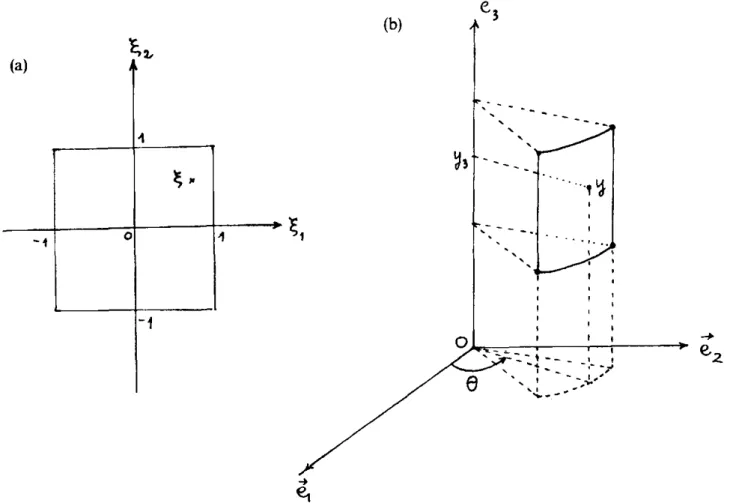
(p, 8) (Figure 2) and in cylindrical co-ordinates, with p constant, (u, v)

=

(8, y_{3 )}

(Figure 3).

2. Interpolation of~

In practice, it is advantageous to obtain the components of the density~ in the local basis which

varies with the pointy of S. For this reason, we attach much importance to the choice of the

co-ordinates system and we will consider different ways to interpolate the components of

q,

in the

local basis. Use will be made of isoparametric elements.

In Cartesian co-ordinates, for instance, the local basis b is invariant; it coincides with the global,

--fixed basis e of the space E _{3 :}

1

~-~" 0 -1 0

...

b) a,)

(b) (a)

.,

~" -1 0

"

-1 ' .... ...

....

' ' ' ' " _' ··--.,~ I I I I 1 ~ ... ~·:.-, _ _ _ I : e2. ' ... 1- - ... ,

e '

_' t - - - I 11, ,

...

"~-_.,""

Figure 3. Interpolation with cylindrical co-ordinates: (a) local co-ordinates ~ = (~ _{1 ,} ~2 ); (b) global co-ordinates (0, y_{3 )}

The density

q,

is considered in the fixed basis:

~=cfJ1e1 +cfJ2e2+t/>3e3

Each of the components of ~ is then interpolated classically by

cPi

= (N (~)){

cPi}

e, iE { 1, 2, 3}

In cylindrical co-ordinates, the local basis varies with the point y:

The density will be considered in the variable basis:

cl»

=

4>

PeP+ l/Joe6

+

¢3 e3

and its components are now interpolated by

cP i

= (

N (e)) { </J i} e, iE{p,

e,

3}

Relations (6) in turn yield

Cn

b { cfJ( e) }

=

b [ .Af ( ~)

J •

C 11 {

cP}

e

(6a)

(6b)

(7) where c, denotes the canonical basis of IR". The letters b, c" added in small characters recall the

fol1ows: Nl 0 0

l

N2 0 0

I

N3 0 0

I

N4 0 0 Cl2

o

1

o

o

I

o

o

I

b[JV (~)] = 0 _Nl Nz N3 0 _N4 0 I I I 0 0 N1 I 0 0 Nz: 0 0 N3 I 0 0 N4 I I

and the density

t1l

in the case of cylindrical co-ordinates can be expressed by

( tP

)e

=

((t/Jp,

t/Jo,

tP3)\

(t/Jp, t/Jo,

¢3)2,

(t/Jp, t/Jo,

¢3)3,

(t/Jp, tPo,

tP3)4)e

One can then express the derivatives of

t1l

with respect to the parameters u and v:

where .d..

=

.4{ . .d.. e 'JI,u u 'JI .d.. = vi( . .d.. e '+', v v 'f' if u =I(} if u

=

0' if v =I(} if v = (}

The matrical representation of .#₁ in the bases b and c₁₂ (case of four-node elements) is

0 -N~

ol

_I 0 -N2

ol

_I 0 -NJ

ol

_I 0 -N4 0 ctz _{I I} I b[Ai'₁ (~)] = _Nt 0 0 1 N2 0 0 I N3 0 01 N4 0 0 0 0

o

I

o

0

o

I

o

0

ol

0 0 0 I l _I

3. Discretization of the integral equation

(8a) (8b)

(9)

We study next how to transform each of the terms of the right-hand side of (4). First, let us consider the terms containing «Jl. u· We have

(cp,u, e, F,Jny0=[cp,u·(er 1\ F,v)]ny0

Similarly

As for the term «11. u 1\

e,

we have

= [(Aucpe)·(er 1\ F.J]nyo (using (8a))

= [ny0 ® A!J (er 1\ F.v)J«Jle (lOa)

(lOb)

(11) where an implicit sum is implied on the repeated subscript iE{l, 2, 3} or {p, (}, 3}, b₀=(b₀

J

is the basis related to y_{0 .} It should be noted that the components of the given stress t(y_{0 ,} ny_{0 )} in the left-hand side of(4) are obtained in the basis b0 . Furthermore, in interacting or surface crack problems,

b0 may differ or not from b, according to the relative position of the particular point y0 and the

ordinary one y. Now in virtue of (11):

In the same manner, the fourh terms of (4) can be expressed by (e,:cl-,u)[(F,v, Dy0 , e,.)e,.+(ny0·e,.)e,. 1\ F,vJ =[((F,v, ny_{0 ,} e,)e,+(ny0·e,.)e,. 1\ F,v)®.AJ e,]cpe

Eventually, relations (10) are expressed in matrical form by

(lOd)

(cp,u, e,, F,v) Dyo

= [ {

Dyo} (

(e,

A F,v) [.A uJ)J { cp }e (12a)

(<J»,u, e,., n,o) F,v = [ {F,v} ((e,. A Dyo) (.A uJ)] { cp }e (12b)

(F,v 'Dyo)cl-,., A e,=(F,v·nyo) [ {bo;} ((e,. 1\ bOi}) [.A.,])] {cp }e (12c)

(e,.·ci>,

11)((F,v, n,0 ,

e;.)e,+(ny

0

·e,.)e,.

A F,v)

(12d) It should be noted that, in (12d) for instance, as the given stress in the left-hand side is expressed in the basis b_{0 ,} the vector e,. between braces { } (column-matrix, see Appendix) must be expressed in the basis b_{0 ,} whereas the same e,. between angle brackets ( ) (row-matrix) must be expressed in the basis b.

The terms containing

«P.

v are discretized in the same manner; they yield relations analogous to

(12) where «P.v takes the place of

<l»,u,

and F,u of F,v·

Thus, for each particular point y₀ of the crack, we have discretized the integral equation using a

tensor formalism, equations (10). This equation being discretized as a vectorial equation, and not

as three separate scalar equations, this formalism allows us a compact programmation for numerical purposes. One has to solve an algebraic system in the form

[A]

{cf>}={B}

where [A] is a full, non-symmetrical matrix,

{4>}

the unknown vector and

{B}

contains the components of the given stresses. In interacting or surface crack problems, {

cf>}

contains different

vector densities corresponding respectively to different cracks or boundaries of the solid !?}.

N.B.: From the dimensional point of view, the matrices appearing in equations (12) (terms between brackets [ ]) are expressed in the inverse of a length or are dimensionless according as Cartesian, polar or cylindrical co-ordinates are involved.

NUMERICAL PARTS

I. Embedded circular crack

First, the program has been tested on the simple case of a circular crack centred at 0, with radius a, under a uniform pressure p, the analytical solution of which is well known:15

8(1-v2)· pa ---~

cp(p)= xE Jt-{p/a)2·e3 , p=

IIOyll

As for any plane crack imbedded in the infinite medium, the three modes are uncoupled. The stress intensity factor in the opening mode is given by

K

₁

=2p~

The natural choice of parameters for the penny-shaped crack is (u, v)=(p, 0). One should notice

the crack edge is especially better shaped than with the usual grid pattern, as shown in Figure 4. Moreover, this choice of parameters facilitates the computation of the stress intensity factors

which require to be taken as a limit when moving along a direction perpendicular to the crack edge.

The given stress vector is expressed at each point Yo in a local basis b₀=(ep_{0 ;} e_{80 ;} e_{3 ),} whereas the vector density

4>

at a pointy in b=(ep; e_{0 ;} e_{3 );} this situation is shown in Figure 5.

Figure 6 represents a quarter of a mesh with 181 interior nodal points (7 nodes along the radius

and 36 along the polar angle (J, each sector being equal to 1 0°). The numerical integration was

performed with 2 x 2 Gaussian points.

As expected, the numerical values of the radial and tangential displacement discontinuities

q,

P

and

¢

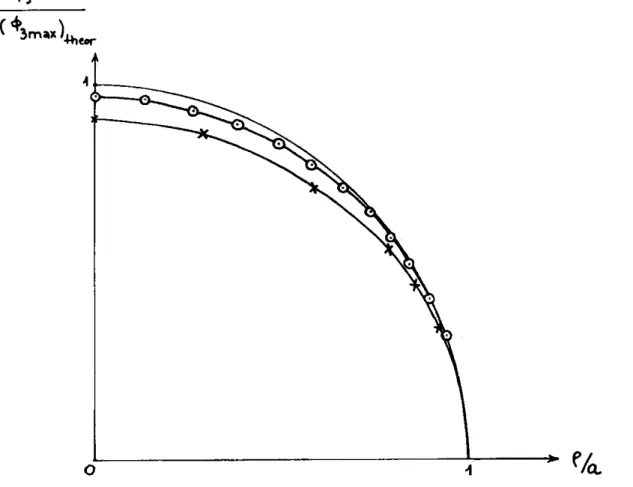
₉ are zero; moreover, all the nodes of the same radius have identical ¢3 values. It is interesting to note that, in mixed modes problems, the formulation herein proposed permits us to obtain directly the radial and tangential components of cf» (l/Jp and c/>_{9 )} without additional calculations, because cf» is expressed in the local polar basis. Table I and Figure 7 give respectively the values of c/>3 normalized by the theoretical maximum value (c/>3max)theor=8(1-v2)pa/nE, and

its curve compared to Sneddon's solution. It should be noticed that one obtains in fact

(a) I I I I I \ \ ---.. /

Figure 4. Circular crack: (a) use of polar co-ordinates (u. v) = (p. 0); (b) usual grid pattern. use of Cartesian co-ordinates

Figure 6. Circular crack: first mesh

Table I. Circular crack. First mesh. c/>₃ values normalized by the theoretical maximum value

0 0·3 0·6 0·8 13/15 14/15 I 1 0·95393 0·8 0·6 0·49889 0·35901 0 0·91244 0·87363 0·72500 0·56512 0·47032 0·35041 0 E/(16n(l-v2

))·c/>₃ directly from the program, so that the Young's modulus E datum is not necessary. The relative error on </>₃ is maximum at the crack centre and equals 8·75 per cent; that of

the computed stress intensity factor K₁ is 3·97 per cent.

Figure 8 represents a finer mesh with 529 interior nodes (13 along the radius and 48 along the polar angel 8, each sector being equal to 7·5°). Use is always made of 2 x 2 Gaussian points.

Table II and Figure 7 give the values of ¢3 normalized by the theoretical maximum ¢rvalue. The

relative error on ¢₃ at the centre is 2·97 per cent; that of the computed stress intensity factor K ₁ is 0· 25 per cent.

2. Semi-elliptical crack in a cylindrical bar under combined loads

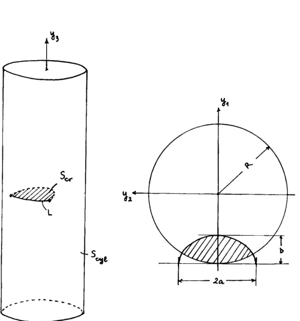
Let us consider a cylindrical bar with radius R, containing a semi-elliptical crack with semi-axes

a

and b. The crack occurs perpendicularly in the lateral surface of the cylinder, along a line which will be referred to as the surface-line of the crack (Figure 9). Three types of loads will be applied uniquely on the crack, the external surface of the bar being left free: a uniform pressure, a linear pressure along the y ₁-axis, and a shear distribution corresponding to the torsion of the bar (Figure 1 0).

According to the discussion in Reference 9, the surface crack problem can be investigated by considering a two crack problem: the first crack is the studied one, the second is a

Figure 7. Circular crack: </J₃ normalized by the theoretical maximum value: analytical results; analytical results; - x - x - computed values with the first mesh; - 0 - 0 - computed values with the second mesh

Figure 8. Circular crack: second mesh

.Sc,: the semi-elliptical crack, admitting the Cartesian parametrization:

Fer: .6,cr3(yl, Y2)-+yEScr .Scyl: the cylinder-shaped crack, admitting the parametrization:

Fcyl: Acyl= [0, 2n[x[ -h, h]3(0, z)-+ yEScyl

. L: the surface-line, which is the intersection of Scyt and the closure of Scr

~~

,

Table II. Circular crack. Second mesh.

4J

₃ values normalized by the theoretical maximum value

0 1 (}13 D-99151 0·26 D-96561 0· 38 0·92499 0·49 0·87172 0·59 0·80740 0·67 0·74236 0·74 0·67261 o-8 o-6 Q-85 D-52678 (}9 (}43589 D-95 (} 31225 1 0

-

-·---

_... ' Q-97028 (}96311 0·93761 0·89805 0·84761 0·78810 0·72839 0·66313 (}59344 (}52047 (}42999 (}31752 0 ~--..2A. - - + t

_..,-

,....

cr'Nll ~ ~ 'tmalC

b· .. ,

' ' ' ' ' ' ' ' '

',

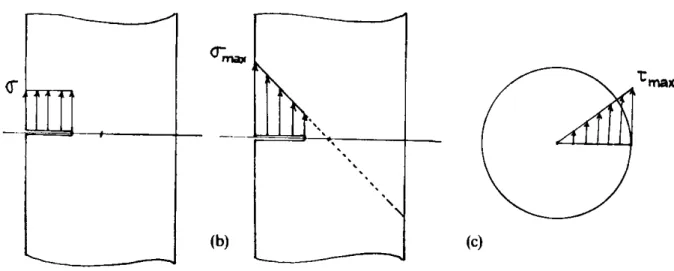
(a) (b) (c)

-Figure 10. Three loading types on the surface crack: (a) uniform pressure; (b) linear pressure; (c) shear distribution resulting from the torsion of the bar (amau •max: maximum stress values)

respectively the unknown density functions over Scr and Scyl · cl-cr ='Per ° F cr' cl»cyl = 'Pcyl

°

F cyl

The edge of Scyt is the union of the upper and the lower crack edges of the cylinder, plus a

vanishing, counterclockwise contour surrounding L. The set of equations of the problem can be

written as follows:

t(y0 ,

ny

0

)=vpf

(kernel containing q,cr)dudv

.lcr

+

f

(kernel containing q,cyl )du dv

Acyl (13a)

t(y0 , ny0)=0=J (kernel containing cl-cr)dudv Acr

+

vp

f

(kernel containing «Pcy1)du dv

Acyl (13b)

lim 'Pcr(Y) = 0 (13c)

Scr3Y--+Y

lim 'Pcyt(Y)

=0

(13d)

Scyl3y-+y

VyEL, lim 'Pcr(Y)+ lim 'Pcy1(y)- lim 'Pcyt(y)=O

Scr3Y--+Y ~;f3y--+ji ~~~3y--+ji

(13e) where the kernels in (l3a) and (13b), given by (4), are not made explicit because of their length; S~~f

and S~~~ denote respectively the upper and lower part of the cylindrical crack, separated by the

section containing Scr· The relation (13e) holds if we choose the normal to Scr upward with respect to the crack and the normal to Scyl outward with respect to the cylinder. With another choice of surfaces orientations, however, this relation still holds but the signs before each term may change. Furthermore, one can easily verify that, in various surface crack problems, one or more relations of type (13e) may be obtained. Relations of type (l3e) allow one to verify that, though every contour integral is different from zero, there always appears a set of thesewhich cancel one another.

For numerical purposes, a crack depth-radius ratio b/R=0·4 and a semi-axes ratio b/a= 5/1 ~0·714 are considered. The cylinder lateral surface is divided into 748 elements with 731 interior nodes, while the semi-elliptical crack contains but 58 elements and 60 interior nodes (Figure 11). So large a node number on the free surface is due to the use of four-node elements with their sides along the parallel of the cylinder or along its axis. It should be wiser to use curved cylindrical elements (i.e. elements with distinct cylindrical nodal values) so as to realize a relatively refined mesh around the surface-line together with a coarse mesh far away, and to reduce notably the node number on the free surface. We have, however, not chosen such elements because of the difficulties caused to automatic mesh generations. In fact, the sole aim of this paper is to show the feasibility and the validity of the proposed approach. Anyway, the interesting feature is the little node number on the crack itself.

Like the previous numerical example, use is made of four-node elements and the numerical quadrature is performed with 2 x 2 Gaussian points. Tables III, IV and V give the 4>rvalues, ie{l, 2, 3}, resulting from three loading types. From Tables III and IV, one can note that, under uniform or linear pressure loadings, the crack is seen to be in the opening mode. Table V shows on the contrary that, under torsion loadings, the crack deforms in a mixed mode II+ III. With the same maximum stress values (i.e. u=umax• see notation, Figure 10), ¢₃-values due to uniform pressures are found to be greater than those due to linear pressure.

It is important to note that one obtains Cartesian components of

q,

over the crack, and cylindrical components on the cylinder. Some interesting results can be deduced from the

<Pi-values, ie { p,

e,

3}, over the free surface. In the opening mode for instance, the point belongs to the upper crack face and located at the centre of the ellipse has, besides a positive ¢_{3 ,} a negative ¢P.

This means that it moves upward with respect to the crack and outward with respect to the cylinder, as to some extent predicted by physical considerations.

Figures 12, 13 and 14 represent the crack in non-deformed and deformed states, where for a better representation deformations are emphasized by a multiplier equal to 5.

It is rather attractive to represent the stress intensity factor variations along the crack edge, but in surface crack problems, the stress intensity factor definition is almost difficult to establish.

0

,

...

,,

ljl; 4; 44 s~ H .2'; 1t (.f

.

.; u. 1

Figure 11. Surface crack mesh: 58 elements, 60 interior nodes. The elements are shaped into the elliptic co-ordinates defined on the ellipse

Table III. Components of E/(16n(l-v2_{))·cPcr resulting from a uniform pressure: ¢}

1 =¢2=0, ¢3#:0;

(v =0·3, b/R =0·4, bja

=

5/7, b= 5, u= 1, the unit of a, b, R is [L], that of u is [F· L-2

], that of the above

components is [F·L - 1_]) E E E E Node 16n(l-v2 ) ·¢3 Node _{16n(l-v2 ) ·¢}3 Node 16tt(l-v2_)·¢3 Node _16n(l-v2)·c/>3 1 0·4658 2 0·4583 3 0·4583 4 0·4351 5 0·4351 6 0·3955 7 0·3955 8 0·3445 9 0·3540 10 0·3745 11 0·3857 12 0·3894 13 0·3857 14 0·3745 15 Q-3540 16 0·3445 17 0·2777 18 0·2838 19 0·2981 20 0·3110 21 Q-3184 22 0·3211 23 Q-3184 24 0·3110 25 (}2981 26 0·2838 27 Q-2777 28 0·2179 29 0·2358 30 0·2503 31 Q-2620 32 0·2681 33 0·2702 34 Q-2681 35 0·2620 36 0·2503 37 0·2358 38 0·2179 39 Q-1554 40 0·1866 41 0·2014 42 0·2110 43 (}2157 44 0·2173 45 0·2157 46 0·2110 47 0·2014 48 O·i866 49 0·1554 50 0·0876 51 0·1358 52 0·1444 53 0·1489 54 0·1500 55 0·1511 56 0·1500 57 0·1489 58 0·1444 59 0·1358 60 0·0876

Table IV. Components of E/(16n(l-v

2

))·cl»cr resulting from a linear pressure with umax = 1:

c/J1

=c/>

₂

=0,

c/J3

#:0

E E E E

Node

16n(1- v2 ). c/>3 Node 16n(1-v2 ) _·c/>3 Node 16tt(l- v2 ). c/>3 Node 16n(l-v2 ) ·c/>3

1 0·3994 2 0·3927 3 0·3927 4 0·3722 5 0·3722 6 0·3371 7 0·3371 8 0·2921 9 0·3018 10 0·3193 11 0·3287 12 0·3317 13 0·3287 14 0·3193 15 0·3018 16 0·2921 17 0·2341 18 0·2394 19 0·2500 20 0·2592 21 0·2643 22 0·2661 23 0·2643 24 0·2592 25 Q-2500 26 0·2394 27 0·2341 28 0·1829 29 Q-1967 30 0·2061 31 0·2129 32 0·2163 33 0·2175 34 Q-2163 35 Q-2129 36 Q-2061 37 0·1967 38 Q-1829 39 0·1300 40 0·1537 41 0·1623 42 0·1669 43 0·1688 44 Q-1695 45 0·1688 46 Q-1669 47 Q-1623 48 Q-1537 49 0·1300 50 0·0732 51 0·1099 52 Q-1134 53 0·1139 54 0·1133 55 0·1135 56 0·1133 57 Q-1139 58 Q-1134 59 Q-1099 60 Q-0732

Table V. Components of E/(16n(l- v2))·_,cr resulting from a torsion shear distribution with tmax=l:c/>3=0, l/J1, c/>2:-#:0 Node E t6n(l-v2) ·c/>1 E 161t(l-v2) ·l/J2 Node E 16n(l-v2 )

·l/>

1 E 16n(1 - v2 )

·l/>

2 1 0·0000 -0·2913 2 0·0074 -0·2858 3 -0·0074 -0·2858 4 0·0125 -0·2698 5 -0·0125 -0·2698 6 0·0135 -0·2431 7 -0·0135 -0·2431 8 0·0099 -0·2107 9 0·0265 -Q-2554 10 0·0234 -0·2758 11 0·0132 -Q-2871 12 0·()()()() -0·2907 13 -0·0132 -0·2871 14 -D-0234 -0·2758 15 -0·0265 -0·2554 16 -0·0099 -0·2107 17 0·0044 -0·1761 18 0·0258 -0·2104 19 0·0352 -0·2334 20 0·0302 -0·2456 21 0·0165 -0·2510 22 0·0000 -0·2528 23 -0·0165 -0·2510 24 -0·0302 -0·2456 25 -0·0352 -0·2334 26 -0·0258 -0·2104 27 -Q-0044 -0·1761 28 -0·0002 -0·1488 29 0·0363 -0·1927 30 0·0413 -Q-2039 31 0·0345 -0·2104 32 0·0185 -0·2120 33 0·0000 -0·2126 34 -0·0185 -0·2120 35 -0·0345 -0·2104 36 -0·0413 -Q-2039 37 -0·0363 -D-1927 38 0·0002 -Q-1488 39 0·0050 -0·1378 40 0·0320 -0·1548 41 0·0394 -0·1640 42 0·0336 -0·1661 43 0·0184 -0·1652 44 ()-()()()() _-0·1648 45 -0·0184 -Q-1652 46 -0·0336 -0·1661 47 -0·0394 -0·1640 48 -0·0320 -0·1548 49 -0·0050 -0·1378 50 0·0016 -0·0972 51 0·0611 -0·1335 52 (}0580 -Q-1193 53 Q-0455 -0·1103 54 0·0222 -0·1024 55 0·0000 -0·1006 56 -0·0222 -0·1024 57 -0·0455 -0·1103 58 -0·0580 -0·1193 59 -D-0611 -0·1335 60 -D-0016 -0·0972

Generally speaking, the elastic state varies from plane strain in the interior to plane stress at the free surface. In the following, we shall limit our consideration to the stress intensity factors at the deepest point of the crack. There exists at this point a plane strain state; in the case of

v

= 0·3,

b/R=0·4, bja=5f7, the stress intensity factors are given by: for a uniform pressure,

=0·820

for linear pressure, K.J(amaxfo) = 1/((Jmaxfo) X

2nj2n

X lim { E/(16n(l-v2))·c/J3/Jr}

r-oo

(a)

(b)

Figure 12. Surface crack under a uniform pressure: c/J1 =c/J2 =0, c/J3 #;0. Crack shapes before and after deformation: (a) front view; (b) spatial view

(a)

reF?/

(b)

Figure 13. Surface crack under a linear pressure: c/J1

=

c/J2 =0, c/J3 #;0. The deformation shape is analogous to that due to a

uniform pressure: (a) front view; (b) spatial view

for a torsion shear distribution,

=

-0·298

(As previously mentioned, E/(16n( I-v2 ))·cb;. i

=

2 or 3, are obtained directly from the program). The stress intensity factors are normalized by u max

fo

or -rmax

fo

related to a slit crack with

Figure 14. Surface crack under a torsion shear distribution: upper view

In Reference 16, stress intensity factors are computed by means of the boundary integral equation method for semi-elliptical cracks in cylindrical bars of diameter equal to 12 mm, in tension or in bending. The crack geometry corresponding to that considered herein is bfa

=2·4 mm/l36 mm=5/7, b/2R=2·4 mm/12 mm=0·2, for which the stress intensity factor can be obtained by interpolation:

in tensile loading with a= 1000 MPa, K1 = 72·62 MPajffi --.K,/(a Jn:b)=0·836

K, =47·10 MPajffi --.KJ!(amaxfo)=0·569 in pure bending with a max= 953·4 M Pa, ·

One can find in Reference 1 7 a list of stress intensity factors for various crack and solid geometries. The so-called surface crack in solid cylinder is studied under tensile loading and pure bending (Figure 15). These actually are almond-shaped cracks which occur perpendicularly to the lateral surface of the cylinder. For lack of matter for comparisons, we consider, however, the crack of this type with b/R =0·4; at the deepest point of the crack, the computed values are expected to be

close to the above ones. The stress intensity factor is then expressed in the additive form 1 7

which yields in tensile loading:

K, =[a· Fo +amu' F1 JJ'i{h

F 0 = G[0·752 + 1·286/J

+

0·37 Y 3 ] F ₁ = G[0·923

+

0·199 Y4] G = 0·92(2/n)·1/cos

fJ·

[tan

fJ

/

fJ]

112 Y= 1-sin/3

fJ

= n:/2 · b/2R K.f(a Jib)= 0·800

and in pure bending: ( K 1 /( (1 max Jib)= 0·606.

Recently, in Reference 18, use is made of the finite element method to study semi-elliptical cracks in cylindrical bars under tensile loadings. When computing the stress intensity factor K_1, the assumption that a plane strain state holds in the neighbourhood of the crack is made in order to apply the virtual crack extension method. Charts for K₁ at the centre of the crack are given for

b/a=O·Ol, 0·2, 0·5, 1·0, 2·0 and for various bfR ratios. An extrapolation from these K₁-charts then gives us approximately the interval containing the K₁/((1J'i{h) ratio: for b/R =0·4, bfa= 5/7, with a

uniform pressure (1, K.f((f J'i{h)e[0·93, 1·00].

·~

2R.

investigations are being pursued to obtain more complete abacuses of stress intensity factors, reported for various crack configurations.

CONCLUDING REMARKS

Equation (4) has been discretized and written in a tensor form, equation (10). Whereas lengthy expressions should be expected if (4) had been dealt with as three separate scalar equations, this approach yields a concise form of the discretized equation and thus allows a compact way of programming. Moreover, a crack parametrization being chosen; this enables one to obtain directly the components ofthe displacement discontinuity vector at each point, as well as the stress intensity factors along the crack edge, in a local basis. Unlike the usual finite element method, no singular element is required near the crack edge. The method herein proposed can also easily be applied to non-symmetrical crack configuration problems for which the boundary integral equation method becomes inefficient. Moreover, since no a priori assumptions of a plain strain or plain stress are to be made, the integral equation method can be used to investigate the stress singularity in the neighbourhood of the crack.

The example on the circular crack shows that one can obtain good results, using only four-node elements and 2 x 2 Gaussian points. The problem of the semi-elliptical crack in a cylindrical bar was also investigated with combined loadings. The numerical results obtained in opening mode were found to be in the range of different existing results for analogous crack geometries. The proposed method also allows one to obtain results for more complex loadings, in particular for torsion loading to which few works in the literature are devoted.

APPENDIX

Notation

b=(b_1;

b

_{2 ;}

b

_{3 )} a local basis at a pointy in E₃ c,. the canonical basis of ~~~

f} the elastic body characterized by constants (E, v) of} the boundary of q)

e=(e_1; e_2; e_{3 )} the fixed basis of E3

E₃ the three-dimensional Euclidean space

F a parametrization of S, defined on a domain A in IR2: A3(u, v)-+ y = F(u, v)ES. In

general, F,u may not be perpendicular to F.v

I unit tensor

ny normal to S at yeS

S the crack surface

as

the crack edge

t(y, n,) stress vector at yeS, with respect to normal.n,

T Kupradze tensor

y, y0 respectively an ordinary, a particular point of S

pvJ., surface integral on S, defined in the principal value sense

{a} column-matrix of components of a vector a in a basis. One may encounter b{ a} which emphasizes the basis bin question

[%] matrical representation of a linear transformation .AI from E3 into IRn, also

Cn

denoted more precisely by e [AI']

=(a " b)·c

(a, b, c)

a®b tensor product defined by Vc E IR3, (a® b)c

=

a(b·c)

REFERENCES 1. T. A. Cruse, Int. J. Solids Struct., 5, 1259-1274 (1969).

2. J. M. Boissenot, J. C. Lachat and J. Watson, Revue Physique Appliquee, 9, 611 (1974).

3. V. D. Kupradze, T. G. Gegelia, M. 0. Bashelishvili and T. V. Burchuladze, Three-Dimensional Problems of the Mathematical Theory of Elasticity and Thermoelasticity, North-Holland, Amsterdam, 1979.

4. H. D. Bui, Compt. Rend. Acad. Sci. (Paris), Serie A. 280, 1157 (1975). 5. T. A. Cruse. AFOSR-TR-0813. 1975, pp. 13-20.

6. P. S. Theocaris and J. G. Kazantzakis, Int. J. Fract., Rl17-R119 (1978). 7. J. Weaver, Int. J. Solids Struct., 321-330 (1977).

8. V. Sladek and J. Sladek, Int. J. Solids Struct., 19, 425-436 (1983).

9. A. Levan and J. Royer, Int. J. Fract., 31, 125-142 (1986).

10. J. G. Kazantzakis and P. S. Theocaris, Int. J. Solids Struct., IS, 203-207 (1979). 11. P. S. Theocaris and J. G. Kazantzakis, Int. J. Fract., R165-R167 (1979).

12. P. S. Theocaris, N. I. loakimidis and J. G. Kazantzakis, Int. j. numer. methods eng., 629 (1980). 13. N. I. loakimids, Appl. Numer. Methods, 1, 183-189 (1985).

14. Liu Jun, G. Beer and J. L. Meek, Eng. Analysis, 2, (3) (1985). 15. I. N. Sneddon, Proc. Roy. Soc. London, 187, 229 (1946).

l(i. A. Athanassiadis, J. M. Boissenot, P. Brevet, D. Francois and A. Raharinaivo. Int. J. Fract., 553-566 (1981).

17. R. C. Forman, V. Shivakumar, J. C. Newman, L. Williams and S. Piotrowski, Fatigue Crack Growth Computer

Program. NASA/FLAGRO, Version June 1985.