Examining Vicinity Dynamics in Opportunistic Networks

HAL Id: hal-00863218

https://hal.archives-ouvertes.fr/hal-00863218

Submitted on 18 Sep 2013

HAL is a multi-disciplinary open access

archive for the deposit and dissemination of

sci-entific research documents, whether they are

pub-lished or not. The documents may come from

teaching and research institutions in France or

abroad, or from public or private research centers.

L’archive ouverte pluridisciplinaire HAL, est

destinée au dépôt et à la diffusion de documents

scientifiques de niveau recherche, publiés ou non,

émanant des établissements d’enseignement et de

recherche français ou étrangers, des laboratoires

publics ou privés.

Examining Vicinity Dynamics in Opportunistic

Networks

Tiphaine Phe-Neau, Marcelo Dias de Amorim, Miguel Elias Campista, Vania

Conan

To cite this version:

Tiphaine Phe-Neau, Marcelo Dias de Amorim, Miguel Elias Campista, Vania Conan. Examining

Vicinity Dynamics in Opportunistic Networks. ACM International Conference on Modeling, Analysis

and Simulation of Wireless and Mobile Systems (ACM MSWiM), Nov 2013, Barcelone, Spain. ACM,

pp.153-160, �10.1145/2512840.2512861�. �hal-00863218�

Examining Vicinity Dynamics in

Opportunistic Networks

Tiphaine Phe-Neau,

Marcelo Dias de Amorim

UPMC Sorbonne Universit«es Paris, France

{

tiphaine.phe-neau,

marcelo.amorim

@lip6.fr

Miguel Elias M. Campista

Universidade Federal do Rio de Janeiro

Rio de Janeiro, Brazil

miguel@gta.ufrj.br

Vania Conan

Thales Communications & Security

Gennevilliers, France

vania.conan@thalesgroup.com

ABSTRACT

Modeling the dynamics of opportunistic networks generally relies on the dual notion of contacts and intercontacts be-tween nodes. We advocate the use of an extended view in which nodes track their vicinity (within a few hops) and not only their direct neighbors. Contrary to existing approaches in the literature in which contact patterns are derived from the spatial mobility of nodes, we directly address the topo-logical properties avoiding any intermediate steps. To the best of our knowledge, this paper presents the first study to ever focus on vicinity motion. We apply our method to several real-world and synthetic datasets to extract interest-ing patterns of vicinity. We provide an original workflow and intuitive modeling to understand a node’s surroundings. Then, we highlight two main vicinity chains behaviors rep-resenting all the datasets we observed. Finally, we identify three main types of movements (birth, death, and sequen-tial). These patterns represent up to 87% of all observed vicinity movements.

1.

INTRODUCTION

Understanding patterns of mobility in the context of opportunistic networks is fundamental for the design of efficient networking protocols and algorithms. The lit-erature in this area has issued a significant number of papers that provide answers to questions related to how nodes meet each other and at which frequency [3, 5, 10]. A common characteristic to these works is that they all rely on the dual notion of contacts and intercontacts. A contact occurs when two nodes are within direct com-munication range of each other, whereas an intercontact is defined as the complementary of a contact, i.e., when two nodes are not in contact.

In our work, we have been advocating that nodes should consider an extended view of their neighbor-hood by including nodes that are not in contact but still nearby in the analyses – nodes that can be reached through a few hops, which we refer to as the

vicin-∗

Work presented at the ACM MSWiM’13 Poster Session, November 4–8, 2013, Barcelona, Spain.

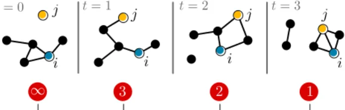
t = 0 t = 1 t = 2 t = 3 i j i j i j i j

distance n between i and j

∞ 3 2 1

Figure 1: An example of vicinity motion knowl-edge. At t = 0, node j is outside i’s vicinity but coming closer. At t = 1, j pops into i’s vicinity at a 3-hop distance. At t = 2, j moved closer to i at a 2-hop distance and even arrives in contact at t = 3.

ity [12]. Understanding how a node’s vicinity behaves may help understanding opportunistic networks under-standing and may consequently improve the resulting routing techniques.

To the best of our knowledge, no previous work has investigated how the vicinity of a node evolves with time. In Fig. 1, we illustrate the evolution of a small network. The traditional contact/intercontact defini-tion would consider the first three time steps as the same, i.e., that i and j are in intercontact. In opposi-tion, we make the distinction between the four situa-tions and we propose to investigate the impact of such new definition by addressing the following questions:

• Given that two nodes i and j are separated by n hops, what is the probability that they be

sep-arated by m hops (m 6= n) when the distance

changes?

• Is it possible to identify patterns in this dynamics so that motion can be predicted?

We model the vicinity motion as simple chain process computed from a data structure containing the evolu-tion of a node’s vicinity, called “timeline”. The idea is to track the vicinity of nodes up to a distance κ. The κ

frontier is tuned according to the monitoring extent re-quired by the system design and the amount of overhead tolerated (as monitoring the vicinity generates some sig-naling overhead). At the end, the network might rely on the measured vicinity motion to make estimations on fundamental parameters such as the delivery delay and social relationships among nodes. We perform several analyses using both real-world and synthetic traces. We make several contributions:

• A model to understand vicinity behavior. We define a node’s neighborhood with the κ-vicinity notion and provide a framework to analyze it with the vicinity motion. We also provide the corre-sponding generating workflow to build vicinity chains which capture the statistical evolution of the dis-tance between nodes.

• Two main network behavior and three move-ment types. The first network type displays ex-tended chains which represent a rich neighborhood with long end-to-end paths between nodes within the κ-vicinity. Whereas the other network type ex-hibits short chains with paths constrained to few hops. For extended chains, we noticed how three types of movements dominate all motions. Birth, death and sequential moves may represent 87% of all observed moves for a given dataset.

The remainder of our paper is organized as follows: in Section 2, we provide the necessary background infor-mation to define a vicinity as well as the vicinity motion definition and the generating workflow. In Section 3, we detail the datasets we use in our study. In Sections 4 and 5, we display our findings. In Section 6, we examine related studies and expose our future works. Finally, in Section 7, we conclude our study.

2.

THE VICINITY NOTION

2.1

Vicinity formalization

The concept of κ-vicinity, which we defined in a com-panion paper [12], is fundamental in this work as it de-fines the extension to which our motion analysis apply. We discriminate a node i’s vicinity according to the number of hops between i and its surrounding neigh-bors.

Definition 1. κ-vicinity. The κ-vicinityVκi of node

i is the set of all nodes with shortest paths at most κ hops from i.

Clearly, _Vi

κ−1 ⊂ Vκi. In Fig. 2, we illustrate the

1-vicinity and 2-1-vicinity for node i.

In our motion analysis, we will focus on movements within a node’s κ-vicinity.

i

i

1-vicinity

2-vicinity

Figure 2: An example of κ-vicinity. Left: node i’s 1-vicinity represents the set of neighbors at a 1-hop distance from i. Right: node i’s 2-vicinity represents the set of nodes at a 2-hop distance from i.

In our work, we make a clear distinction between nodes that are not in direct contact but still have a path connecting them and nodes that have no possi-bility of communication (i.e., there is no path between them) [11]. A pair of nodes are in favorable intercon-tact of parameter n when they are exactly at a shortest n-hop distance. Two nodes at a 1-hop distance are in contact. We formally define favorable and pathless in-tercontact as follows:

Definition 2. Favorable intercontact. An inter-contact is considered as “favorable” with parameter n when there is a contemporaneous shortest path of length n separating the two nodes under consideration, where {n ∈ N∗ _{| 2 ≤ n < ∞}.}

Definition 3. Pathless intercontact. In opposi-tion to favorable situaopposi-tions, “pathless” intercontact in-dicates the lack of end-to-end paths between a pair of nodes, i.e., n_{→ ∞.}

We investigate movements happening from contact or any given n favorable intercontact to any other possi-ble state. This analysis will help us understand how a node’s κ-vicinity behaves.

2.2

Vicinity motion: methodology and outcomes

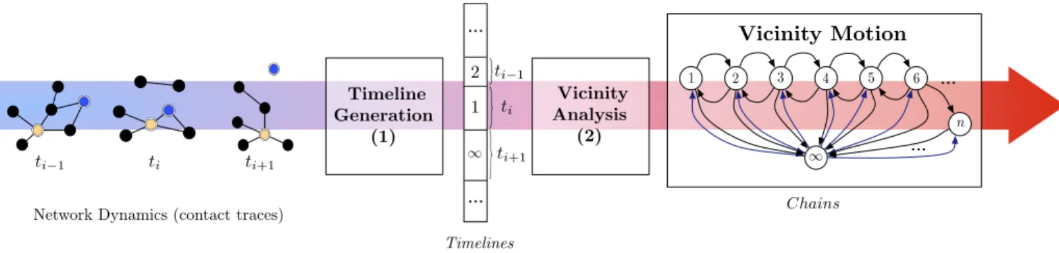
More than what happens far from a given node, vicin-ity motion considers all movements within a node’s κ-vicinity. We provide elements to answer the following question: when the distance n between nodes i and j change, what is the probability that their distance be-come m, m _{6= n? We refer to the period between two} changes in the distance as a step. To answer this ques-tion, we follow a two step methodology and present the whole workflow in Fig. 3:

1. Timeline generation. From the previous step, we compute a vicinity timeline, which is the pro-gression of shortest distance between any two nodes

Network Dynamics (contact traces) Timelines Chains ∞ ... ... 1 2 3 4 5 6 n Timeline Generation (1) Vicinity Analysis (2) ti−1 ti ti+1 1 2 ∞

}

}

}

Figure 3: Vicinity Motion generation workflow. We begin by reading Network Dynamics under the form of contact traces describing network connectivity through time. We process them using (1) the timeline generation module. This stage produces timelines. Step (2) aka Vicinity Analysis examines these sequences to compute transitional probabilities and corresponding vicinity motion chains.

1 2 3 4 5 6 7 50 51 52 53 54 Num b er of hops Time (×103_seconds)

Figure 4: A pairwise timeline from the Unimi dataset. From 50,000 seconds to 50,500 seconds, the two nodes did not have a path to one an-other. Then, they briefly were at a 5-hop dis-tance before coming closer at a 4-hop and then a 3-hop distance and so on.

through time (see Fig. 4 for an example). By us-ing these timelines we are able to perform various probabilistic analyses. To better focus on our ob-servations, we will not be detailing the timeline generation process here.

2. Vicinity analysis. Timelines provide the nec-essary information to characterize the transition probabilities between given distances.

We model vicinity motion through a chain process for each pair of nodes. For a given node i, let Xs

i,j be the

variable representing the distance between nodes i and j at step s. The vicinity analysis step takes timelines as inputs and provides the corresponding transitional probabilities for vicinity chains.

0.06

0.44

0.38

0.24

0.16

0.30

0.31

1

2

3

4

0.25

0.22

0.19

0.28

0.30

0.33

0.36

Figure 5: Infocom05 average vicinity motion for a pair (i, j) and κ = 4. For the sake of clarity, we display only a few transitions. The

probabil-ity of a node appearing in contact _{{∞ → 1} is}

6% or when nodes are at a 3-hop distance, the probability for them to be next at distance 2 is 30%.

States. The chain states depends on the κ we choose, i.e., the size of the vicinity we wish to monitor. The number of states is κ + 1; the first state, denoted ‘∞’, corresponds to the case where the two nodes are in path-less intercontact (see Definition 3). The state_{1} repre-sents a contact and the remaining states_{{2, . . . , M = κ}} correspond to a situation of favorable intercontact of the corresponding length (see Definition 2).

Note that we consider each pairwise movement as a step unit. We do not consider specific time frame dura-tions to avoid dataset dependence.

Transitional probabilities. To understand vicinity motion, we focus on the transitional rates between states, i.e., the probability of two nodes being at a distance of m at step s knowing that they were at a distance n in the previous step: P(Xs

i,j = m | X s−1

i,j = n), m 6= n.

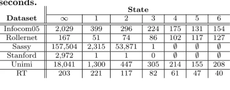
This informs us exactly on the movements within the vicinity. The average durations spent in each state are given in Table 1.

As an example, we show in Fig. 5 the average transi-tional probabilities of vicinity motion for Infocom05, a dataset collected at IEEE Infocom 2005 containing the contacts observed among 41 nodes (see Section 3 for more details on this dataset). For the sake of clarity, we omit certain transitions. As we can see, when nodes i and j are in pathless intercontact (_{∞), the} probabil-ity that they meet directly is 6% while it is 25% for a favorable 3-hop intercontact.

3.

DATASETS

We analyze vicinity motion in real-world experiments and a synthetic dataset (denoted by an (S)) described hereafter.

Infocom05 measurement was held during a conference in 2005 [2]. 41 attendees carried iMotes collecting infor-mation about other iMotes nearby within a 10m wireless range. We study a 12-hour interval bearing the highest networking activity. Each iMote probes its environment every 120 seconds. Infocom05 represents a professional meeting framework.

Rollernet had 62 participants measuring their mutual connectivity with iMotes during a 3 hour rollerblading tour in Paris [16]. These iMotes sent beacons every 30 seconds. This experiment shows a specific sport gath-ering scenario.

Unimi is a dataset captured by students, faculty mem-bers, and staff from the University of Milano in 2008 [4]. They involved 48 persons with special devices probing their neighborhood every second. Unimi provides a scholar and working environment scenario.

Stanford has 789 persons in a high school carrying TelosB motes – detecting contacts up to a 3m range [15]. Salath´e et al. gave Motes to students, teachers and staff members for a full day. For computational reasons, we focus on a subset of 200 participants. Motes send beacons every 20 seconds. Stanford has a settings with a majority of teenagers who have a tendency to dwell in groups of interests.

Sassy was held in the Saint Andrews University by researchers who used 27 T-motes to capture contacts among alumni and scientists [9]. The T-motes broad-casted beacons every 6.67 seconds over a 79 days period. Sassy brings a sparser academic setting during a wider time frame.

RT (S) is a mobility model correcting flaws from the Random Waypoint model [8]. We sampled the behavior of 20 nodes following this model on a surface of 50 x 60 m2 _{with speed between 0 and 7 m/s and a 10m range.}

This surface simulates an office-wide setting.

Table 1: Average time spent in each state in seconds. State Dataset ∞ 1 2 3 4 5 6 Infocom05 2,029 399 296 224 175 131 154 Rollernet 167 51 74 86 102 117 127 Sassy 157,504 2,315 53,871 1 ∅ ∅ ∅ Stanford 2,972 1 1 0 ∅ ∅ ∅ Unimi 18,041 1,300 447 305 214 155 208 RT 203 221 117 82 61 47 40

Table 2: Stationary distributions in percentage.

State Dataset ∞ 1 2 3 4 5 6 7 Infocom05 25.3 5.5 15.4 20.0 16.0 9.7 5.1 2.2 Rollernet 28.2 2.3 7.7 11.5 12.5 11.5 9.5 7.3 Sassy 49.2 34.8 15.5 0.5 0.0 0.0 0.0 0.0 Stanford 45.0 48.0 6.9 0.3 0.0 0.0 0.0 0.0 Unimi 35.0 9.0 14.0 15.0 12.0 8.0 4.0 2.0 RT 29.1 5.0 10.6 14.1 14.3 11.5 7.7 4.5

4.

VICINITY CHAINS

4.1

Average time spent in each state

Table 1 presents the average duration spent in state κ in seconds for each state. For RT and Unimi, we observe a gradual decrease of durations. On the other hand, Rollernet has an increasing tendency while In-focom05 has a mixed behavior. The specific status of Rollernet as a dynamic sport events may explain the increasing values. Short distances have a very low life span because of the fickle and dynamic connectivity in the setting. The crowd absorbs longer distances (note that we do not discriminate path changes if they are of the same length).

4.2

Stationary distributions

In Table 2, we show the stationary distributions for the different datasets when κ = 7. In Infocom05, when we come across the setting, there is a 25.3 % chance that the node we are looking for will not belong to our κ-vicinity, 5.5 % chance of the node being in contact, 15.4 % at a 2-hop distance, 20% at a 3-hop, and so on. Note that by observing its 4-vicinity, we have a 77% chance of spotting a node we are actually looking for. Such a posteriori knowledge is useful to evaluate the probability of finding a node quickly upon arrival or even to quantify the probing frontier in order to keep low maintenance costs.

4.3

Short and extended chains

We observe two types of vicinity chains. Extended ones that can travel up far to states like 10 or 12 or shorter ones with movements only up to 1 or 2 hops.

4.3.1

Short chains

Short chains almost join the previous assumption that nodes are either in contact or in pathless intercontact; the difference here is that they can drift to a 2-hop dis-tance. We noticed such setting for two of our datasets: Sassy and Stanford. The observed chain consists in states_{{∞, 1, 2}. As a result, such settings bear no or} very low favorable intercontact advantages. Most of times, when you detect a node, its next move will al-most always be to vanish from the vicinity. Opportunis-tic protocols must also take these patterns into account when necessary.

4.3.2

Extended chains

Datasets like Infocom05, RT, Rollernet, and Unimi display extended vicinity chains (see Fig. 5 for an ex-ample). Extended chains bear more potential traveling states. Some even going to 12 and longer distances. Extended chains have the characteristic to allow high favorable intercontact states and, therefore, the possi-bility of wider end-to-end transmissions via recurrent favorable intercontacts. Extended chains may also ex-hibit a wide range of intra chain movements. We will next see how three types of movements dominate ten-dencies. With only a few movement patterns, we will show it is possible to oversee most of a node’s upcoming movements.

5.

VICINITY INSIGHTS

Datasets bearing extended chains offer more possi-bilities of next hop transitions. In the datasets we analyzed, we observe three main types of transitions, namely birth, death, and sequential movements.

5.1

Birth in the

-vicinity

We qualify of birth the phenomenon of appearance in the κ-vicinity after a period of pathless intercontact. The main interest of such knowledge is for a node or a protocol to know at which distance another node may appear. Imagine in the Infocom05 dataset that node i wants to send a message to node j, who is currently out-side i’s κ-vicinity, without relying on fully opportunistic forwarding. Given the computed stationary values from Fig. 5, we now know that j will appear with a proba-bility of 25% at a 3-hop distance.

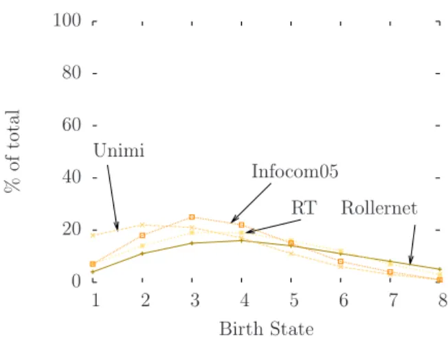
In Fig 6, we present the values concerning the birth motion for our datasets. On the x-axis, we represented the actual incoming state (the distance at which a node appears). On the y-axis, we present the actual birth transitional probability for each distance. For all datasets, the highest birth probability belongs to the set {1, 2, 3, 4_{}. The cumulated transitional probabilities up to 4} represent from 50% to 70% depending on the datasets. For a random dataset, if we had chosen to extend these probing limits only to a state 4, we would detect from

0 20 40 60 80 100 1 2 3 4 5 6 7 8 % of to ta l Birth State Rollernet Unimi RT Infocom05

Figure 6: Proportion of birth values. 50% to 70% of nodes vicinity appearance. Hence, prob-ing your 4-vicinity is enough to get most of the arrivals patterns in a node’s surrounding. We confirm our pre-vious finding on the optimal limit of κ-vicinity prob-ing [13].

5.2

Death in the

-vicinity

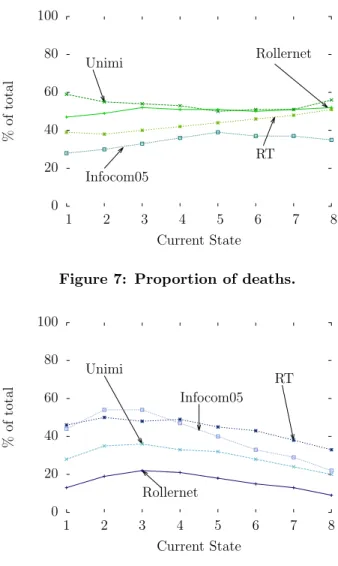
In opposition to the notion of birth for arrival pat-terns, we call death the phenomenon of nodes vanishing from the κ-vicinity. We analyze the datasets in two dif-ferent aspects: the proportion of deaths with regard to the full chain (absolute) and compared to natural move-ments only (which excludes transitions between non-consecutive states except toward_∞).

In Fig. 7, we show the evolution of death probabil-ities for the different states of the chain. All datasets have quite steady absolute death rates, their absolute maximum variation being 12%. Being able to foresee death movements ie. a node being in pathless intercon-tact can indicate when to begin a fully opportunistic routing technique. As long as nodes are in the vicinity, we can use end-to-end paths towards them. However, when we suspect that nodes will next be out of the κ-vicinity, it may be time to trigger a different routing approach.

5.3

Sequential movements

We define as sequential movements for two nodes the process of drifting closer or further from each other us-ing adjacent states of the chain: when nodes (i, j) are at a 4-hop distance, they sequentially move closer if they are at a 3-hop distance during their next step, they sequentially drift away if they are next at a 5-hop dis-tance.

Our first observation is that a non-negligible part of vicinity movements stems from sequential behaviors. For Unimi and Infocom05, as long as nodes stay in the κ-vicinity, sequential movements represent between

0 20 40 60 80 100 1 2 3 4 5 6 7 8 % of total Current State Rollernet Unimi RT Infocom05

Figure 7: Proportion of deaths.

0 20 40 60 80 100 1 2 3 4 5 6 7 8 % of total Current State Rollernet Unimi RT Infocom05

Figure 8: Proportion of sequential movements. 50% and 87% of movements. Another observation is that the further two nodes are, the higher the propor-tion of erratic movements (all movements that are nei-ther birth, nor death, nor sequential). However, sequen-tial movements still rule.

Wider vicinity bear fickler connectivity at the edges and more random hops. We call erratic behavior or random movements, all movements that are not birth nor death nor sequential moves. They represent a mi-nor share of vicinity motions and can be overlooked as predicting their destination is tougher and brings only marginal knowledge gains.

6.

RELATED AND FUTURE WORK

To characterize and analyze networks, researchers used contact traces collected during real-life measurements. However, due to the lack of extensive realistic traces, re-searchers had to create synthetic mobility models and generated the corresponding contact traces. By cre-ating different mobility models, they emulated human

0 20 40 60 80 100 1 2 3 4 5 6 7 8 % of to ta l Current State

Death Sequential Erratic

Figure 9: The vicinity motion movements repar-tition (death, sequential and erratic) for Info-com05. Death and sequential movements rep-resent the greater part of all possible outgoing movements.

behaviors to test protocols they designed in specific set-tings [8, 7]. Other studies moved towards accurate con-nectivity rebuilding based on real-life contact traces [17]. All these analyses uncorrelated node behaviors from their surrounding. With the vicinity motion patterns, we try to bridge the gap between these points. Now, more than understanding the whole network movements, we can see the patterns followed by a node’s vicinity. Using specific DTN monitoring mechanism would im-prove opportunistic detection abilities [14].

We are aware that our datasets may not be long enough to conduct time frame analysis but we under-stand that this parameter may have a deep impact on our observations. However, our main observations as well as our method remain valid. In a future work, we plan on integrating this parameter in our analyzer im-plementation to define the accurate time window size by performing time frame analysis as seen in [6].

We next plan on developing a timeline generator. The generator would integrate the identified vicinity pat-terns (birth, death, sequential movements) and allow multiple types of contact traces generation. It would also allow vicinity analysis of user generated traces fol-lowed by the generation of traces with similar charac-teristics with various size scales. An effort has already been made to directly generate contact traces based on contact and intercontact analyses [1]. Yet, it lacked the neighborhood notion we bring with the vicinity motion patterns.

7.

CONCLUSION

In this paper, we present the value of nodes’ vicin-ity and their neighbors in opportunistic networks. We

presented an approach to model a node’s vicinity using the κ-vicinity notion and a system workflow to under-stand its inherent behavior. This workflow generates useful information like timelines and transitional proba-bilities. Timelines allow pairwise distance analysis while transitional probabilities detail how nodes move rela-tively to each other. Our study found out that there are two main types of vicinity chains: extended and short chains. We discriminate each type according to the at-tainable states in the chain. Another finding showed the dominance of only a few move types within the network. These moves, namely birth, death and sequential cover up to 87% of all movements patterns. To understand how these moves evolve according to the current states of the node, we also quantified the evolution of each of the identified movements. Vicinity motion patterns help us understand how a neighborhood behaves which is fundamental in opportunistic networking. But it also presents an overall timeline pattern that can be useful to predict node’s potential next moves as well as a lead in the direction of a new type of realistic connectivity generation.

Acknowledgment

Tiphaine Phe-Neau and Marcelo Dias de Amorim car-ried out part of the work at LINCS (http://www.lincs.fr). This work was partially funded by the European Com-munity’s Seventh Framework Programme under grant agreement no. FP7-317959 MOTO. Miguel Elias M. Campista would like to thank CNPq, Faperj, CAPES, and FINEP for their financial support.

8.

REFERENCES

[1] R. Calegari, M. Musolesi, F. Raimondi, and C. Mascolo. CTG: A Connectivity Trace Generator for Testing the Performance of Opportunistic Mobile Systems. In ACM SIGSOFT Symposium on the Foundations of Software Engineering, Dubrovnik, Croatia, Sept. 2007.

[2] A. Chaintreau, P. Hui, J. Crowcroft, C. Diot, R. Gass, and J. Scott. Impact of human mobility on opportunistic forwarding algorithms. IEEE Transactions on Mobile Computing, 6(6):606–620, 2007.

[3] V. Conan, J. Leguay, and T. Friedman.

Characterizing Pairwise Inter-contact Patterns in Delay Tolerant Networks. In International Conference on Autonomic Computing and Communication Systems, Rome, Italy, Oct. 2007. [4] S. Gaito, E. Pagani, and G. P. Rossi.

Fine-Grained Tracking of Human Mobility in Dense Scenarios. In IEEE Conference on Sensor, Mesh and Ad Hoc Communications and Networks, Rome, Italy, June 2009.

[5] M. C. Gonzalez, C. A. Hidalgo, and A.-L. Barabasi. Understanding individual human mobility patterns. Nature, 453(7196):779–782, June 2008.

[6] M. Latapy and C. Magnien. Complex network measurements: Estimating the relevance of observed properties. In IEEE Infocom, pages 1660–1668, 2008.

[7] M. Musolesi and C. Mascolo. Designing mobility models based on social network theory.

SIGMOBILE Mob. Comput. Commun. Rev., 11:59–70, July 2007.

[8] S. Pal Chaudhuri, J.-Y. Le Boudec, and M. Vojnovic. Perfect Simulations for Random Trip Mobility Models. In IEEE Infocom, Miami, Florida, USA, Aug. 2005.

[9] I. Parris, G. Bigwood, and T. Henderson. Privacy-enhanced social network routing in opportunistic networks. In IEEE International Conference on Pervasive Computing and Communications, Mannheim, Germany, Mar. 2010.

[10] A. Passarella and M. Conti. Characterising aggregate inter-contact times in heterogeneous opportunistic networks. In IFIP Networking, Valencia, Spain, May 2011.

[11] T. Phe-Neau, M. Dias de Amorim, and V. Conan. Fine-Grained Intercontact Characterization in Disruption-Tolerant Networks. In IEEE

Symposium on Computers and Communication, Kerkyra, Greece, June 2011.

[12] T. Phe-Neau, M. Dias de Amorim, and V. Conan. Vicinity-based DTN Characterization. In ACM MobiOpp, Zurich, Switzerland, Mar. 2012.

[13] T. Phe-Neau, M. Dias de Amorim, and V. Conan. The Strength of Vicinity Annexation in

Opportunistic Networking. In IEEE International Workshop on Network Science For

Communication Networks (Netscicom), Torino, Italy, Apr. 2013.

[14] V. Ramiro, E. Lochin, P. Senac, and R. Thierry. On the limits of DTN monitoring. In IEEE WoWMoM Workshop on Autonomic and Opportunistic Communications, page 6, Madrid, Spain, June 2013.

[15] M. Salath´e, M. Kazandjieva, J. W. Lee, P. Levis, M. W. Feldman, and J. H. Jones. A

high-resolution human contact network for infectious disease transmission. PNAS, 107(50):pp. 22020–22025, 2010.

[16] P.-U. Tournoux, J. Leguay, F. Benbadis, J. Whitbeck, V. Conan, and M. D. de Amorim. Density-aware routing in highly dynamic DTNs: The rollernet case. IEEE Transactions on Mobile Computing, 10:1755–1768, 2011.

[17] J. Whitbeck, M. Dias de Amorim, V. Conan, M. H. Ammar, and E. W. Zegura. From encounters to plausible mobility. Pervasive and Mobile Computing, 7(3):206–222, Apr. 2011.