D
OCUMENT DE
T
RAVAIL
DT/2001/16
Parental Income and School
Attendance in a Low-Income Country:
a semi-parametric analysis
PARENTAL INCOME AND SCHOOL ATTENDANCE
IN A LOW-INCOME COUNTRY : A SEMI-PARAMETRIC ANALYSIS
Denis Cogneau
(DIAL-UR CIPRE de L’IRD) e-mail : cogneau@dial.prd.fr
Eric Maurin (CREST-INSEE)
Document de travail DIAL / Unité de Recherche CIPRE
Novembre 2001
RESUME
Utilisant des données sur trois générations successives de Malgaches, nous construisons un nouvel estimateur semi-paramétrique de l’effet du revenu parental sur la décision de scolariser les enfants. Nous proposons de nouveaux tests de biais de simultanéité et d’hérédité affectant les estimations usuelles de cet effet. Nous révélons l’importance du premier type de biais : selon nos estimations, en prenant insuffisamment en compte la simultanéité des processus de formation de revenu et des décisions de scolarisation, la littérature existante sous-estime l’effet réel des ressources familiales sur les décisions d’envoyer ou non les enfants à l’école.
ABSTRACT
Using data covering three successive generations of Malagasy people, we construct a new semi-parametric estimator of the effect of parental income on the decision to send children to school. We propose new tests of simultaneity and hereditary biases affecting the usual estimates of this effect. We reveal the importance of the first type of bias. Our estimates show that the existing literature underestimates the real effect of family resources on decisions as to whether or not to send children to school by not taking enough account of the simultaneity of income formation processes and schooling decisions.
Index
1. INTRODUCTION...2
1.1 Simultaneity biases and hereditary biases...3
2. THE THEORETICAL FRAMEWORK...5
2.1 Extensions ...7
3. ECONOMETRIC SPECIFICATIONS...8
3.1 The identification problem...9
3.2 A semi-parametric estimator ...11
4. THE RESULTS AND THEIR INTERPRETATION ...13
4.1 Parental income and delayed schooling...15
4.2 Parental income and non-schooling...17
4.3 Extension: the effect of child labour...18
5. CONCLUSION ...19
REFERENCES...20
Appendices Index
Appendix A: The schooling condition ...23Appendix B: Test for the existence of simultaneity and hereditary biases...24
Appendix C: Presentation of the data and construction of the variables...26
Tables Index
Table 1: The extent of schooling of Malagasy children and adolescents in 1993: Some descriptive statistics...29Table 2: Effect of parental income on the probability of starting school at six years old ...30
Table 3: Effect of parental income on the probability of never being schooled...31
Table 4: Effect of parental income on the extent of schooling of adolescents aged 15 to 17: a semi-parametric estimate (auxiliary variable: day of the year in which the child is born)...32
Table 4bis: Effect of parental income on the extent of schooling of adolescents aged 15 to 17 years: a semi-parametric estimate (auxiliary variable: primary school density) ...33
Table 5: Effect of parental income on the extent of schooling of adolescents aged 15 to 17 years: a parametric estimate (ordered Tobit)...34
1. Introduction
Despite being historically and culturally quite school-orientated, Madagascar’s level of schooling is currently one of the lowest in the world. One Malagasy child in …ve never goes to school1. The majority start school one to two years later than the
normal age. Many children then leave school early and rare are those who attend secondary school. Madagascar is not an isolated case. The same phenomenon can be seen in most of the sub-Saharan African and South Asian countries2. Children
in poor countries today generally still receive little or no schooling with the result that one of the basic conditions for economic development is left unful…lled.
Obviously, it is very important to understand the underlying reasons for the extremely low level of schooling among children in low-income countries. From a strictly economic point of view, the reasons can be found in both the lack of school infrastructures (insu¢cient supply) and the lack of family resources (insu¢cient demand). When parents have no or virtually no means of borrowing to …nance their children’s studies, the lower the family income the lower the level of the children’s schooling. This paper concentrates mainly on this second aspect of the problem. To what extent does the lack of household resources explain the extremely low level of schooling in low-income countries? How sensitive is a family’s educational demand to its income? We have a wealth of Malagasy data at our disposal to identify the real impact of parental income on schooling decisions. These data show the rates of school attendance across three successive generations (children, parents and grandparents). Based on these data, we make a two-part contribution:
(a) In terms of method, we construct a new semi-parametric estimator of the e¤ect of parental income on the decision as to whether to send children to school. We use the new estimator for qualitative response model with endogenous regres-sors recently introduced by Lewbel (2000). We propose new tests of simultaneity biases and hereditary biases a¤ecting the usual estimates of this income e¤ect.
(b) In terms of …ndings, we reveal the importance of the simultaneity biases a¤ecting usual estimates of the income e¤ect on schooling decisions. We …nd that the existing literature greatly underestimates the real e¤ect of family resources on schooling decisions by not taking enough account of the simultaneity of the income formation processes and schooling decisions. In the Malagasy case, our work interprets the low level of schooling as one of the direct consequences of
1See Cogneau et al. (2000).
the poverty and inequalities that became rooted in the country with the economic collapse of the early 1980s. Despite the country’s having a long-standing tradition of schooling children and despite the large investments made to improve and mod-ernise school infrastructures in the pre-recession years, the lack of resources has placed school out of the reach of a considerable proportion of Malagasy families.
1.1. Simultaneity biases and hereditary biases
A large body of research has already addressed the impact of income on school-ing decisions in the developschool-ing countries. However, we believe that this question has still not been perfectly answered. The main problem is that the correlations observed by the surveys between parental income and the level of children’s school-ing are merely an indirect and potentially biased re‡ection of the real impact of income on schooling. There are at least two reasons for this.
The …rst reason is the simultaneity of schooling decisions and work organisation and production decisions in the family. Certain factors simultaneously determine family income and whether or not it is worth schooling the children3. In the
presence of such factors, the gross correlations between income and schooling are a¤ected by a bias that can be called a simultaneity bias.
A second kind of problem has to do with family resources and skills passed on from generation to generation. Where these factors are received by the par-ents, they determine the family’s productivity and current income. Where they are passed on to the children, they a¤ect schooling decisions either by raising the anticipated return on schooling or by raising the anticipated return of training the children up on the family trade. In the presence of such factors, the cor-relations between income and schooling could be as much the manifestation of unobserved resources transmitted from parents to children as the manifestation of a real income e¤ect on schooling.
In general, the existing literature essentially endeavours to reduce the hered-itary biases, i.e. the biases caused by resources transmitted from generation to generation and unmeasured by the surveys. One of the most frequently used econometric strategies is to analyse schooling and school performance di¤erences between descendents of a same lineage4. Berhman and Wolfe (1987) use data
col-3Assuming that the occupational skills acquired by parents over their life are at least partially
passed on to the children. When these skills are substitutes for educational skills, the most skilled parents in their trade are both those with the highest incomes and those with the least interest in sending their children to school.
lected in Nicaragua to analyse the di¤erences in the number of years of schooling between pairs of cousins (whose mothers are sisters) as a function of observed dif-ferences in income and education between their parents. They …nd no signi…cant relation between the observed schooling and resource di¤erences. They conclude from this that the generally observed correlations between parental income and children’s schooling derive from unobserved abilities and resources passed on from generation to generation.
Another method consists of simultaneously analysing the parents’ schooling and their children’s schooling based on data covering a number of generations. Lillard and Willis (1992) use Malaysian data covering four generations to simul-taneously estimate a schooling transition model for parents and children without excluding the possibility of a correlation between the unobserved determinants of the parents’ transitions and the children’s transitions. Assuming residual nor-mality and exogenous parental income, they conclude that the parents’ education in‡uences the children’s education. Yet they do not identify any signi…cant income e¤ect5.
This paper takes a new look at the impact of income on the level of schooling by endeavouring to formalise and reduce both hereditary biases and simultaneity biases. We simultaneously analyse the parents and children’s education, but also the parents’ income based on data covering three generations. We center our analysis on a single transition6 (the …rst of whether to go to school), but develop
semi-parametric estimation techniques without any restrictive assumption about the residuals.
The article is structured as follows. First, we explain the theoretical framework in which our econometric work can be situated (Section 2). We then detail our econometric speci…cations and the semi-parametric estimators used (Section 3). Next, we describe the results of our estimates (Section 4). The data used are described in detail in Appendix C.
and Corcoran, Jenks and Olneck (1976).
5As the authors themselves say, the e¤ect of parental income is nevertheless hard to interpret
in the Lillard and Willis analysis (1992): a certain number of variables potentially linked to income (such as the quality of the dwelling) are also used as control variables. For a description of the problems posed by the joint estimation of the income e¤ect and variables potentially linked to income, see, for example, Blau (1999).
6In so doing, we avoid the basic problems of non-parametric identi…cation of transition models
2. The theoretical framework
Generally speaking, our theoretical framework is part of the family of models with an imperfect credit market pioneered by Becker and Tomes (see, for example, Becker and Tomes, 1984). We consider dynasties (indexed by i) that are each made up of an in…nite succession of generations (indexed by t). Each generation experiences two periods of …rstly living with its parents’ generation and secondly living with its children’s generation. In each period, the parents determine the allocation of income between current consumption and educational investment in order to maximise the discounted welfare of the succession of generations. A key point in this is the limited access to credit: the parents cannot contract debts on behalf of their children7. Given this framework, if we denote U(x) as the utility
function, then the objective of dynasty i’s generation t is written:
max E
1
X
k=0
¯t+kU (Cit+k) (2.1)
subject to: Cit+k+ cSit+k = Yit+k and Yit+k = F (Sit+k¡1; uit+k¡1; "it+k);
where Yit is the income of the parents of generation t, Cit their level of
con-sumption and Sita dummy variable that takes the value 1 if the parents send their
children to school. The random variable uit¡1 measures the quality of non-school
resources passed on by generation t ¡ 1 to generation t and "it measures
genera-tion t’s intrinsic productive capacity. Given that we can always rede…ne "it as the
residual of its projection on uit¡1, "it can be assumed to be orthogonal to uit¡1.
Function F is a production function. It describes how income is produced from formal and informal human capital. Parameter b is a discounting coe¢cient while parameter c measures the cost of sending one’s children to school. It corresponds to the schooling costs (e.g. transport and clothing). It also corresponds to the loss of earnings since the children at school contribute less to the family’s work8.
In each period, the optimal schooling choice S¤
it¡1depends on the formal (Sit¡1)
and informal (uit¡1) resources derived from the previous generation and the
cur-rent productivity parameter "it. We can therefore write Sit¤ = S¤(Sit¡1; uit¡1; "it):
For each period, we can also de…ne the optimal level of consumption C¤ it as a
function of Sit¡1; uit¡1 and "it, where,
7This could be interpreted as the consequence of a social norm whereby it is not possible to
force an adult to reimburse a debt contracted by his or her parents.
Cit¤ = C¤(Sit¡1; uit¡1; "it) = F (Sit¡1; uit¡1; "it)¡ cS¤(Sit¡1; uit¡1; "it):
In this model, sending children to school involves a loss of current consumption and hence a decrease in current welfare,
L(Yit) = U(Yit)¡ U(Yit¡ c) ¸ 0 (2.2)
Assuming that U is concave, the lower current income Yit the greater the loss
L(Yit). The poorer the family, the more sensitive it is to the immediate cost of
schooling. The decision to school also entails a welfare gain for generation t + 1, whose discounted value is written,
Git = ¯E(U (C¤(1; uit; "it+1))¡ U(C¤(0; uit; "it+1))¸ 0:
Insofar as the "it+1 shock is independent of past history, the anticipated gain
Git depends on the current period only via the intermediary of uit and can be
rewritten G(uit). Children are sent to school if the immediate losses do not exceed
the anticipated gains, i.e. L(Yit)· G(uit). Given that L decreases, this …rst-order
condition is rewritten,
Sit= 1, Yit ¸ L¡1(G(uit)) = Z(uit) = zit (2.3)
For any given uit; condition (2.3) means that only the families with a high
enough current income will see a point in sending their children to school. In this model, any exogenous increase in poor families’ current incomes reduces the proportion of families under their schooling threshold zit. The aim of this paper
is speci…cally to identify this income e¤ect and test the extent to which redistrib-ution aimed at the poorest families might increase the level of education of future generations.
If uitcould be deemed orthogonal to uit¡1and "it, then zitwould be orthogonal
to Yit and there would be no real identi…cation problem. The di¤erences in the
schooling rates of families with di¤erent incomes would be representative of the real impact of income on schooling9.
9For each level of income Y , the survey’s given estimate of the proportion of schooled
chil-dren among families with income Y would directly give an estimator of Fz(Y ), where Fz is the
distribution function of thresholds zit: Knowing the distribution of thresholds zit in the
popu-lation and knowing that this distribution is independent of income, there would be no problem estimating the impact on schooling of any change in the distribution of income.
The di¢culty with the identi…cation problem is due to the fact that we cannot a priori exclude the existence of links between uit¡1and uitor between "itand uit10.
When such links are present, incomes Yit are correlated with thresholds zitand the
income e¤ect can no longer be identi…ed from the observation of just the Sit and
Yit. Once variables Yit and zit are intercorrelated, schooling di¤erences between
di¤erent income groups re‡ect both the income e¤ect and the fact that di¤erent income groups have di¤erent schooling thresholds zit. Given these circumstances,
identifying the real e¤ect of current income requires more than a simple analysis of the observed correlations between income and schooling. Before moving onto our proposed solution to this identi…cation problem, we will develop two possible extensions of our basic model to broaden the scope of empirical applications and possible interpretations of the e¤ect of income on schooling.
2.1. Extensions
The model developed in the previous section simpli…es the schooling question to the extreme, since there are only two possible options: school the child or not. An immediate extension is to assume not just 2, but K possible degrees of investment in schooling. Variable Sittakes its values not in f0; 1g, but in f0; :::; Kg. Denoting
ck as the cost of an investment Sit= k and setting down c0 = 0, we can de…ne for
all k ¸ 1:
Lk(Yit) = U(Yit¡ ck¡1)¡ U(Yit¡ ck);
the marginal loss of current utility associated with the decision Sit = k and:
Gikt= ¯E(U (C¤(k; uit; "it+1))¡ U(C¤(k¡ 1; uit; "it+1));
the marginal gain expected from this investment, where C¤(k; u
it; "it+1)
repre-sents the optimal consumption in t + 1, conditional on an investment Sit = k in
t.
Assuming that U(x) is concave in x, ck is convex in k and Yit is concave in
Sit¡1, we verify that the current marginal loss Likt increases with k while the
anticipated marginal return Gikt decreases with the schooling investment. In this
10Variables u
it¡1 and uit potentially represent two successive forms of the same technical
and/or cultural assets. Insofar as the culture and techniques passed on from one generation to the next only change slowly over time, uit¡1and uithave a good chance of being intercorrelated.
Variables "it and uit characterise the same adults (i.e. the parents of generation t). They are
determined in the same context and in the same period of time. There is also good reason to think that these two variables are intercorrelated, for example, because parents with speci…c informal know-how (strong "it) can pass their trade onto their children at home without sending
context, each family chooses either not to invest in school (if Gi1t ¡ Li1t · 0)
or the highest schooling investment among those whose net return Gikt¡ Likt is
positive. Denoting zikt as the threshold corresponding to L¡1k (Gikt); and setting
down by convention zi0t = 0 and ziK+1t = 1; we verify that the series of Zikt
increases and that the decision Sit = k is equivalent to (zikt · Yit < zik+1t). The
extent of investment in schooling can therefore be analysed very simply using a multinomial model.
In the basic model, educational investment costs are completely exogenous. Another possible extension of the basic model is to assume that schooling di¢cul-ties can vary from one family to the next depending on exogenous characteristics such as the child’s gender and his or her actual age when schooling becomes compulsory (i.e. as an indicator of his or her maturity). Testing this type of assumption is simply a question of testing whether the schooling threshold varies from one family to the next in accordance with the gender and age of the children. It is also possible to assume that the return on education varies with the parents’ level of schooling Sit¡1. The idea here is that the parents with basic
education might be in a better position to help their children bene…t from school. Adopting this type of assumption is tantamount to assuming that Yit depends
not only on Sit¡1, uit¡1 and "it, but also on Sit¡2. In this context, we can easily
check that the anticipated gains and schooling thresholds vary both in line with the resources uit transmitted from generation to generation and with the parents’
education Sit¡1. In the econometric application, we propose a number of tests of
this assumption that the parents’ educational capital has a direct e¤ect on the probability of schooling the children. In general, we reject it and conclude that the e¤ect of the parents’ schooling on decisions to school the children is in itself weak.
3. Econometric speci…cations
To specify our empirical models, we assume that production function F combines schooling capital (Sit) with the other forms of productive resources (uit) in line
with a technology with a constant elasticity of substitution. We also assume that utility U is concave and homogenous (i.e. U(x) = x® with ® 2 [0; 1] )
and that the costs of schooling remain low against income. In this framework, the …rst-order approximation of L(Yit) is ¯½Y0®exp(Áuit), while Git approximates
¯½Y®
0 exp(Áuit), where ½ represents the return to education and Á a constant whose
capital and the other forms of productive resources (see Appendix A). Based on these assumptions, the schooling decision can be written,
Sit= I(a ln Yit+ bXit+ Áuit); (3.1)
where I(x) is a dummy function that takes the value 1 whenever x is positive and where we have assumed that the relative costs of schooling, i.e. ln(¯½
c ); vary
exogenously from one family to the next and can be written as a linear combination of the variables Xit observed in the surveys. The problem is how to identify a,
given that we also have,
ln Yit = cSit¡1+ uit¡1+ "it: (3.2)
3.1. The identi…cation problem
Before describing the di¤erent estimators used, we will brie‡y outline our identi-…cation strategy and the procedures used to test the validity of this strategy. For the sake of simplicity, we temporarily drop index i and temporarily assume that St can be treated as a linear function of ln Ytand Xt. In the following section, we
explain the conditions that render valid this linearisation of our problem. Based on these assumptions, relations (2.1) and (2.2) give rise to a system of linear relations between education and income,
St = aYt+ bXt+ Áut;
Yt = cSt¡1+ ut¡1+ "t;
St¡1 = aYt¡1+ bXt¡1+ Áut¡1;
Yt¡1 = cSt¡2+ ut¡2+ "t¡1:::
where (to reduce the notations) Yt now represents the logarithm of income.
The problem posed is how to estimate parameter a. Given the dynamic structure of the links between education and income, the ”right” strategy for estimating a clearly depends on the variance-covariance structure of residuals ut and "t. A
number of cases can a priori be envisaged.
(i) In the …rst case, utis orthogonal to "tand ut¡1and all their past realisations
(i.e. E(ut"t¡k) = E(utut¡1¡k) = 0; for all k¸ 0). This is the simplest case where
what is passed on from parents to children (ut¡1) is correlated neither with what
productive capacities ("t). Based on these assumptions, E(Ytut) = 0 and there is
no particular identi…cation problem. A simple regression can be used to estimate the income e¤ect. The correlations between Yt and Stgive an accurate idea of the
real impact of Yt on St.
(ii) In the second case, ut is orthogonal to ut¡1 and "t¡1 (and their past
reali-sations), but not to "t. In this case, there is a link between the parents’ intrinsic
productive ability (i.e. skills acquired during life) and what they pass onto their children, in particular by contributing to their occupational training. In this case, Yt is no longer necessarily orthogonal to ut and the correlation between Yt and St
is a potentially biased estimator of the e¤ect of income on schooling ut¡1:
In this same case, however, St¡1 (parents’ education) has the dual property
of being correlated with Yt without being correlated with ut (i.e. E(St¡1ut) =
E(utut¡1) = 0). The income e¤ect can therefore be identi…ed using St¡1 as an
instrumental variable and all the lineage’s performances previous to St¡1, i.e. Yt¡1;
St¡2, etc.
(iii) If utis orthogonal to ut¡2and "t¡1(and all their past realisations), but not
ut¡1 or "t, then St¡1 becomes potentially correlated with ut and is no longer an
instrumental variable usable to identify the impact of Yt. However, Yt¡1
(grand-parents’ income) remains a valid instrument as do all the previous performances, especially St¡2.
(iv) If ut is orthogonal to ut¡2 and "t¡2 (and all their past realisations), but
not ut¡1 or "t¡1, then Yt¡1 is no longer a good instrumental variable, but St¡2
(grandparents’ education) still is as are all the previous performances.
Our problem in choosing between the di¤erent estimators and instrumental variables is obviously that we do not know the real variance-covariance structure of the non-school determinants of income (i.e. ut and "t). The main asset we
have to help us solve this problem is our wealth of data. These data can be used to measure the current educational investment (St), the parents’ income and
education (St¡1 and Yt), and the grandparents’ education (St¡2). They can also
be used to measure the grandparents’ professional status (farmer, employee in the formal sector or worker in the informal sector), which we can consider to form an indirect measurement of the grandparents’ income level (Yt¡1).
We can use the information on the education and income of three successive generations to estimate the impact of Yton Stin four di¤erent ways: without using
an instrumental variable procedure, using the parents’ education as an instrument, using the grandparents’ income as an instrument, and using the grandparents’ education as an instrument.
If the structure of the residuals corresponds to case (i), then the four estimates clearly have to give the same result. If the structure of the residuals corresponds to case (ii), then only the three instrumental regressions should give the same results. The overidenti…cation tests should not reject the hypothesis of the consistency of instruments St¡1; Yt¡1 and St¡2. If the structure of the residuals corresponds
to case (iii), then only instruments Yt¡1 and St¡2 should be consistent, while in
case (iv), Yt¡1 and St¡2 are no longer necessarily consistent. In other words, by
comparing the results obtained using the four di¤erent instruments available, we can test the extent to which certain conditions necessary for the absence of a hereditary bias or a simultaneity bias may or may not be satis…ed.
In general, these conditions are necessary, but not su¢cient. The structures of the possible residuals need to be speci…ed in more detail in order to express su¢cient conditions for the absence of simultaneity and hereditary biases. In Appendix B, we detail the case in which the residuals are combined in line with a composed error model uit = ui + µ"it. This speci…cation is simple enough
to be used to construct tests and general enough for the di¤erent forms of bias to be combined. In this framework, testing for the absence of a simultaneity bias is tantamount to testing whether µ = 0 and testing for the absence of a hereditary bias comes down to testing whether ¾2
u = 0, where ¾2u represents the
variance of the …xed dynasty e¤ects. In Appendix B, we show that a necessary and su¢cient condition for the existence of a simultaneity bias and the absence of a hereditary bias is that the estimates obtained using St¡1; Yt¡1and St¡2, and even
(St¡1¡ St¡2) as instrumental variables produce the same results and that these
results are di¤erent from those obtained by the ordinary least squares technique.
3.2. A semi-parametric estimator
In this paper, we look at the decision as to whether or not to school children. The dependent variable is a dummy variable and the model considered is not a linear model, but a binary choice model. In this framework, the problem of identifying the income e¤ect is more complicated than suggested by the previous discussion. In the linear case, identi…cation calls simply for an observation of an instru-mental variable Zt in the usual sense such that E(Ztut) = 0 and E(ZtYt) 6= 0:
These conditions are no longer su¢cient in the case of the binary choice model. A fair amount of literature has recently been developed to explore the di¤erent complementary hypotheses whereby the identi…cation of the e¤ect of an endoge-nous explanatory variable becomes possible again in a non-linear model (see the
Blundell and Powell survey, 2000). This paper draws on Lewbel’s recent contri-bution, which we feel to be particularly well suited to our problem and the data at our disposal11. Lewbel (2000) quite generally shows how to identify the e¤ect
of an endogenous explanatory variable Yt in a binary choice model of the form
St = I(a ln Yt+ bXt+ ut), where Xt is a set of exogenous variables. The method
used is to observe (a) an instrumental variable Zt (i.e. such as E(Ztut) = 0 et
E(ZtYt) 6= 0) and (b) an explanatory variable x0t in Xt that is continuous12 and
such that the distribution of ut conditionally on ln Yt and Xt is independent of
x0t.
In our case, the problem of identifying the e¤ect of family income on the decision to school is the same as an identi…cation problem in a linear model when an exogenous and continuous determinant of the decision to school children is observed.
Lewbel (2000) moreover establishes that, in the case whereby an exogenous and continuous x0t variable is observed, the e¤ect of the endogenous variable is
identi…ed by applying the usual estimation techniques using the instrumental vari-ables method to the linearised model LSt = aYt+bXt+Áut;where LStcorresponds
to St¡ I(x0t > 0) divided by the density of x0t conditionally on (X1t; Zt), where
X1t corresponds to Xt minus x0t.
In other words, once we can observe a continuous and exogenous determinant of the decision to send children to school, the problems of identifying and estimating parameter a are exactly the same as those analysed in the previous sub-section by replacing St with its linearisation LSt.
In our speci…c case, there are at least two possible candidates for x0t. The …rst
is the child’s date of birth in the year. This variable can reasonably be assumed to be exogenous. It determines the child’s level of maturity on the date on which he or she can start school. For a given age group (in the school institution sense), the later in the year the child is born, the younger he or she is and the smaller his or her chances of being schooled. Of the children aged 6 to 8 when the survey was taken, 41% of those born in the …rst half of the year started school when they were supposed to as opposed to only 32% of those born in the second half of the year (Table 1). Obviously, the older the children considered, the less noticeable the e¤ect of the date of birth on schooling. Of the teenagers aged 15 to 17 when
11Maurin (1999) applies Lewbel’s estimator to the analysis of repeating years of primary school
based on French data covering several generations whose structure is close to ours.
12The interval of variation of x
0t also has to be broad and (even if it means rede…ning the
the survey was taken, 21% of those born in the …rst half of the year had never been to school as opposed to 18% of those born in the second half of the year. Given the size of the sample, the deviation is signi…cant, but small.
In other words, the date of birth in the year provides a de…nitely pertinent yardstick for the semi-parametric analysis of the e¤ect of income on the age at which children start school. However, it is less suited to providing a gauge of the e¤ect of income on the total length or total absence of schooling. A second candidate for x0t is the quality and density of school infrastructures in the region
in which the child lives. Our survey can be used to reconstitute the number of primary schools per child aged 6 to 15 in the child’s commune (”fokontany”). This variable is continuous and a priori represents a schooling factor13. The problem
is that parents may make decisions to move to another region to be closer to school infrastructures. In other words, it is not certain that the infrastructure density available to the children is completely exogenous to the schooling process studied. However, the survey we use contains the data needed to determine the region in which parents have lived before their migration14. We hence construct
an indicator (DPit) that measures the density of primary schools for the place in
which the parents spent their childhood (if they have not moved) or before any migration (if they have moved). This variable is determined before the schooling process and the formation of current income. It can therefore be considered to be an exogenous measurement of the way in which the school supply quantity has in‡uenced the schooling of the Malagasy children studied. Over 30% of the children aged 15 to 16 in families with a DPit below the median have never been
schooled. Only 9% of the 15 to 17 year old children of families with a DPit above
the median have never been schooled (Table 1).
4. The results and their interpretation
In this section, we present an econometric analysis of the impact of income on the decision to school children, applying the identi…cation and estimation strategies described in sub-sections 3.1 and 3.2. The construction of the samples and vari-ables used for this analysis are detailed in Appendix C. We have estimated four series of models, each corresponding to a particular choice for variable St or for
13The e¤ects of school infrastructures have often been underscored, especially by Lavy (1996)
and Glewwe and Jacoby (1994).
14Appendix C details the construction of this variable and the other variables used in the
auxiliary variable x0t required for the construction of the semi-parametric
estima-tor. The …rst series of models concentrates on the schooling of children aged 6 to 8 at the time of the survey. Variable St takes the value 1 if these children started
school at 6 years old and 0 if not15. In 1993, over 60% of Malagasy children aged
6 to 8 did not start school when they became old enough to do so (Table 1). The second series of models analyses the schooling of teenagers aged 15 to 17 when the survey was taken. Variable St takes the value 1 if they attend school or have
already been schooled, and 0 if not. This variable identi…es those who will never go to school or, in any case, never under normal circumstances. Approximately 20% of the children had never been schooled even though they were old enough to be at secondary school. They will therefore never really be schooled. The third series of models studied analyses these same teenagers aged 15 to 17. This time, however, the models are trichotomic. Variable St takes three values: 0 if they
have never been schooled, 1 if they were schooled for 1 to 4 years (i.e. shortened primary schooling) and 2 if they have already been schooled for more than 4 years. In the …rst three series of estimates, the only explanatory variables consid-ered are the child’s gender, parental income (in logarithm form) measured by the household’s consumption expenditures16, and the child’s date of birth. This
last variable is used as a reference auxiliary variable for the construction of the semi-parametric estimator17. In the fourth series of regressions, we take the
mea-surement of the density of the school infrastructure (of the region in which the father grew up) as a reference auxiliary variable and compare the results obtained with this reference to those obtained using the date of birth (Table 5).18
For each of the four di¤erent types of model, we provide (a) an ordinary least
15A great deal of recent work has more speci…cally focused on analysing not exactly the total
number of years spent at school, but the moment at which the decision is made to start school and then the moment at which the decision is made to attend school less and less regularly. Glewwe and Jacoby (1995) study the role of malnutrition in decisions to delay starting school. Jacoby (1994) studies the importance of indebtedness constraints on the timing of starting and gradually leaving school. More recently, DeVreyer et al (1999) and Bommier and Lambert (1999) have emphasised the role of informal skills that can be acquired in the family before starting school.
16The models have also all been estimated taking the income reported when the survey was
taken as a measure of family income, i.e. a more direct measurement of family income, but also less well measured and more approximate than spending. The …ndings (not reported) obtained from this measurement are very similar to those obtained using spending.
17The estimated e¤ects should be considered relative to the e¤ect of the date of birth. 18Here, the estimated e¤ects should be appreciated relative to the e¤ect of this infrastructure
squares (OLS) estimate of the income e¤ect, (b) an estimate using the father’s schooling as an instrument, (c) an estimate using both the father and grandfa-ther’s schooling and testing the extent of these two instruments’ consistency using Hausman and Sargan tests, (d) an estimate based on the di¤erence between the father and grandfather’s schooling. We also provide the results of the regressions (using the least squares technique and the instrumental variables technique) intro-ducing the amount of the father’s schooling as an additional regressor and using the grandfather’s professional status (taken as an indicator of his income level) as an additional instrumental variable.
4.1. Parental income and delayed schooling
Model (1) in Table 2 corresponds to the ordinary least squares estimate of the e¤ect of income on the probability of being schooled at 6 years old. This es-timate con…rms what the statistics suggest: there is a signi…cant link between parental income and the probability of starting school on time. This OLS estima-tor is only valid to the extent that both hereditary and simultaneity biases can be disregarded. Model (2) corresponds to the instrumental variables technique re-estimation of parameter a using the father’s extent of schooling as an instrumental variable. This estimator remains exposed to the hereditary bias, but escapes the simultaneity biases. The e¤ect of parental income re-estimated in this way is three times higher (^aiv1 = 0.62) than the e¤ect estimated by the ordinary least squares
technique. In addition, the di¤erence between the two estimators is signi…cantly di¤erent to zero19. This …nding suggests that the usual estimators obtained by
the OLS technique are a¤ected by relatively large simultaneity biases and tend to underestimate the income e¤ect. Some unmeasured variables positively a¤ect income and negatively a¤ect the probability of being schooled.
To evaluate the magnitude of the hereditary biases, we have re-estimated the income e¤ect by introducing the grandfather’s length of schooling as an instru-ment in addition to the father’s schooling (Model 3). We have also instruinstru-mented income using the di¤erence between these two variables (Model 4). Each of these two estimators provides signi…cantly higher results than the initial OLS estima-tor. Moreover, the results are neither signi…cantly di¤erent from one another nor
19This estimate shows that a 50% parental income di¤erence is equivalent to an age di¤erence
of 0.6 x 0.5 = 0.3 years at the time when schooling becomes compulsory. Given that the deviation in schooling probabilities between the youngest and oldest children in their age group is 25 points, a 50% increase in parental income implies a 7.5 point increase in the probability of the children being schooled at the normal age.
signi…cantly di¤erent from the estimator obtained by taking the father’s length of schooling as the only instrument. Furthermore, overidenti…cation tests do not reject the hypothesis of the consistency of the two father and grandfather’s edu-cation instruments.
In general, these …ndings are consistent with the assumption that the heredi-tary biases can be disregarded. If we accept that residuals uit can be represented
as the combination of a …xed e¤ect (dynastic ui) and a purely generational e¤ect,
we can unambiguously conclude that there are no hereditary biases (see the analy-sis developed in Appendix B). The only potentially large source of biases therefore looks to be the simultaneity of schooling decisions and income formation processes. In addition to the diagnosis on the relative importance of the di¤erent forms of endogeneity biases, these preliminary estimates also show that the father’s length of schooling (like the grandfather’s) can be considered to be exogenous to the process of schooling the children. To complete this …rst series of models, we have therefore re-estimated models (1) and (3) by introducing the father’s length of schooling as an additional regressor so that its e¤ect can be compared with that of parental income. The ordinary least squares analysis suggests that the di¤erence in the probability of schooling between children whose father went to secondary school and the other children (i.e. 0.35) is signi…cantly greater than the di¤erence in the probability of schooling caused by a doubling of income (i.e. 0.13). Remembering that parental income is endogenous and potentially negatively correlated with residual uit, this least squares estimator of the e¤ect of
the father’s schooling is therefore potentially biased. The bias a priori takes an opposite sign to that a¤ecting the estimator of the parental income e¤ect20.
The instrumental variables technique analysis (i.e. using the grandfather’s length of schooling and the grandfather’s industry as instruments of the e¤ect of parental income) provides quite a di¤erent …nding to the least squares analysis. It con…rms that the real e¤ect of parental income is signi…cantly higher than suggested by the naïve OLS analysis, but also con…rms that the e¤ect of the father’s length of schooling is overestimated by the OLS estimator. Once the question of simultaneity is taken into account, the father’s length of schooling has
20If Á represents the direct e¤ect of S
t on St+1 in Model (5) and bÁmco its OLS estimate, we
verify that: Bs= E(bÁmco¡ Á) = (R 0 tSt)(R0tut) (S0 tSt)2¡(R0tSt)2 = BR °0 1¡°0
where BR is the bias a¤ecting the OLS estimator of the parental income e¤ect and °0 is the
OLS estimator of the return on education. The Bsbias a¤ecting the OLS estimator of the e¤ect
no signi…cant e¤ect as such on the children’s length of schooling. Note that this …nding is in keeping with the theoretical framework developed in the previous sections, but is at odds with the literature that posits that children’s schooling is …rst and foremost a cultural problem.
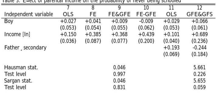
4.2. Parental income and non-schooling
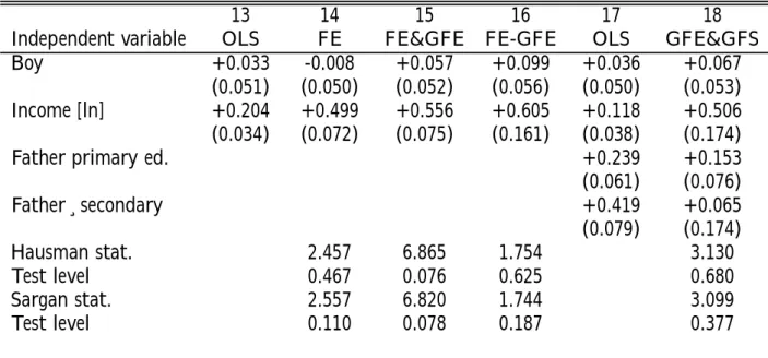
The second series of models (Table 3) analyses the probability of never having been to school by the age of 15. The third series (Table 4) corresponds to trichotomic models analysing the breakdown of children aged 15 to 17 between those who have never been to school, those who have not attended school enough to attain normal primary schooling, and those who have spent more than four years at school. These two series of models hence more explicitly address the evaluation of the e¤ect of income on the process of non-schooling. They provide generally similar results consistent with those obtained regarding delayed entry into school: - The ordinary least squares regressions …nd a signi…cant statistical link be-tween the children’s length of schooling and parental income;
- The instrumental variables technique regressions provide mutually consistent estimates that are higher again than the estimates obtained using ordinary least squares. They reject the hereditary bias hypothesis, but suggest that simultaneity biases may exist biasing the naïve estimates towards zero;
- The addition of the father’s length of schooling as an extra regressor does not change the …nding regarding the e¤ect of parental income on the children’s schooling. In general, the e¤ect of a doubling in parental income (i.e. ¢ ln(R) ¼ 1) is signi…cantly higher than the advantage of having a father who went to secondary school, since this advantage is not signi…cantly di¤erent from zero (see models (6) and (12)).
The fourth series of regressions draws on a new auxiliary variable: the density of primary schools in the commune of origin (see Section 3.2 above for the exact de…nition). This variable captures the way in which the quantity and distribution of school infrastructures across the territory may have in‡uenced the schooling processes. Table 4(b) presents the …ndings of the semi-parametric estimates using the density of primary schools instead of the date of birth as the auxiliary variable. This series of regressions provides qualitatively similar …ndings to the previous series21. The e¤ect of parental income appears to be wholly signi…cant in both
21In terms of point estimations, the …ndings suggest that a 50% increase in an average
the least squares regressions and the instrumental variables technique regressions. The hereditary biases again appear negligible. Even if the estimates are not as accurate, the simultaneity biases still seem to prevail.
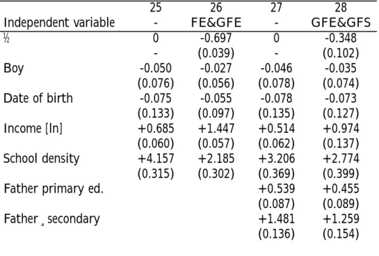
To wind up, we re-estimated the models presented in tables 4 and 4(b) based on the assumption of residual normality (Table 5). In this parametric framework, our model has a Tobit model structure. A …rst equation describes parental in-come as a function of the instrumental variables used (typically, the grandfather’s schooling). A second equation describes the schooling process as a function of parental income and the residuals of these two equations are assumed to comply with a bivariate normal law. The estimators correspond to maximum likelihood. In general, this parametric approach provides results consistent with those previ-ously obtained using semi-parametric estimators. Compared to the coe¢cients of the other variables, especially the auxiliary variables, the parental income e¤ect more than doubles when the father and grandfather’s schooling are used as in-struments22. This …nding still holds when the father’s schooling is included as an
additional regressor and when the grandfather’s schooling and industry are used as sole instruments23. The correlation coe¢cient ½ estimated for the bivariate
nor-mal distribution takes a negative sign, con…rming the nature of the simultaneity biases a¤ecting the naïve estimation of the income e¤ect.
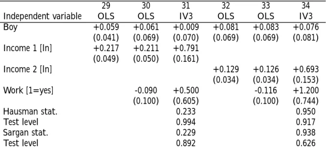
4.3. Extension: the e¤ect of child labour
The model developed in Section 2 does not explicitly introduce child labour as a possible alternative to schooling. In fact, including child labour changes nothing in the theoretical analysis except that (a) the schooling costs are taken to include the losses of current earnings due to sending the children to school rather than to work, (b) parental income (i.e. variable Yt) is taken to be the parents’ income excluding
the children’s contribution. Based on the assumption that child labour is not a marginal phenomenon and given that we only observe total income in the surveys, our main explanatory variable is potentially a¤ected by a measurement error. Rather than using Yt as a regressor, we actually use Yt+ ht, where ht represents
the children’s contribution. In this framework, the ordinary least squares estimate
might be prompted by an increase in the school supply of 0.25 x 0.5 = 0.125 primary schools per child, i.e. approximately 15 points.
22In this non-linear framework, using the grandfather’s education as the instrument means
using the grandfather’s education as an explanatory variable in the equation explaining parental income, without using it in the equation explaining schooling.
of the e¤ect of income on schooling potentially su¤ers from a measurement error bias, whose e¤ects are similar to a simultaneity bias tending towards zero. In other words, the simultaneity biases shown by our previous analyses are potentially interpreted as measurement error biases. To test this interpretation, we have used the information available on child labour in our survey by introducing, as an additional regressor, a dummy variable taking the value 1 if the child works and zero if not. In 1993, 15% of children aged 7 to 8 had worked in Madagascar over the year. In general, the ordinary least squares regressions con…rm that child labour is negatively correlated with a child’s length of schooling, even though the e¤ect is poorly estimated and not signi…cantly di¤erent from zero (Table 6, models 30 and 33). Its e¤ect disappears totally when this variable is instrumented along with parental income. However, the re-estimation of the parental income e¤ect does not change.
5. Conclusion
In this paper, we develop a fairly general detection and recti…cation methodology for the bias that could a¤ect the estimation of the e¤ect of parental income on the decision to send children to school. Our estimates show that the main source of bias comes from the simultaneity of the decision to school children and the parental income formation process. Certain factors not measured by the surveys increase the parents’ productivity and income and simultaneously undermine the sense of sending children to school. These factors are typically the skills that can be informally passed from one generation to the next without the need for schooling. The greater these skills, the more productive the parents and the less point they will see in investing in formal education for their children. Given the existence of these factors, the gross correlation between family income and the probability of schooling children tends to underestimate the causal e¤ect of income on schooling. Neutralising the e¤ect of these factors means that we have to considerably re-estimate up the income e¤ect.
In the Malagasy case, the ”real” e¤ect of income seems to be quite considerable overall. A 50% drop in parental income results in an approximately 20-point decrease in the probability of sending children to school. A good deal of the drop in primary schooling in Madagascar since the early 1980s can therefore be explained not so much by the dilapidation or lack of school infrastructures, but more by the degeneration in household incomes and the spread of poverty due to the economic slump in the early 1980s.
In the planet’s poorest countries, especially in sub-Saharan Africa, universal primary schooling for children is still a remote goal at the end of a long, hard road. In many countries, the schooling situation is now stagnating and sometimes even deteriorating. At …rst glance, the children in these countries are more excluded from the education system when they come from poor families. Our study’s …nd-ings suggest that this problem could be partially solved by a reasonable increase in the redistribution e¤ort to help the poorest families and a reduction in the most extreme forms of inequality. The question nonetheless remains open as to how exactly this redistribution e¤ort could be put into practice. There are many potential ways in which income a¤ects the decision to school children. More in-come means better nutrition, better housing, better health and the ability to get around more easily. It is the extent to which these fundamental problems are better solved that dictates whether the family can envisage investing more in the formal education of their children.Future research should help identify which of the basic goods are politically most likely to be redistributed and economically most e¢cient to redistribute in order to promote a long-term development of education and standards of living.
References
[1] Becker G. S. and N. Tomes, 1984, Human Capital and the Rise and Fall of Families, Journal of Labor Economics, 4, S1-S39.
[2] Behrman J.R. and B. L. Wolfe, 1987, Investments in Schooling in Two Gen-erations in Pre-revolutionary Nicaragua, Journal of Development Economics, 27, 395-419.
[3] Blau D.M., 1999, The E¤ect of Income on Child Development, The Review of Economics and Statistics, Vol LXXXI, n±2;261-277.
[4] Blundell R. and J. Powell, 2000, Endogeneity in Nonparametric and Semi-parametric Regression Models, Unpublished Manuscript, University College London, University of California at Berkeley.
[5] Bommier A., S. Lambert, 2000, Education Demand and Age at School En-rollment in Tanzania, Journal of Human Resources, vol. XXXV, n±1.
[6] Cameron S.V and J.J. Heckman, 1998, Life Cycle Schooling Decisions, Jour-nal of Political Economy,
[7] Chamberlain, G. and Z. Griliches, 1975, Unobservables with a variance Com-ponent Structure: Ability, Schooling and the Economic Success of Brothers, International Economic Review, 16, 2, 442-449.
[8] Cogneau D., J.-C. Dumont. P. Glick, M. Raza…ndrakoto, J. Raza…ndravonona , I. Randretsa, F. Roubaud (2001), Pauvreté, dépenses d’éducation et de santé, le cas de Madagascar, OECD Development Centre, forthcoming. [9] Corcoran M., C. Jencks and M.R. Olneck, 1976, The E¤ects of Family
Back-ground on Earnings, American Economic Review, 66, 430-435.
[10] De Vreyer Ph., S. Lambert, Th. Magnac, 1999, Educating Children: A Look at Household Behavior in Côte d’Ivoire, mimeo CREST & INRA-LEA, 50 pp.
[11] Filmer D., and L. Pritchett, 1999, The E¤ect of Household Wealth on Educa-tional Attainment: Evidence from 35 countries, Population and Development Review, 25, 1, 85-120.
[12] Glewwe P. and H. Jacoby, 1994, Student Achievement and Schooling Choice in Low-Income Countries, Evidence from Ghana, Journal of Human Re-sources, vol. XXIX, n±3.
[13] Glewwe P. and H. Jacoby, 1995, Delayed Primary School Enrollment and Childhood Malnutrition in Ghana, An Economic Analysis, LSMS Working Paper n±98:
[14] Jacoby H., 1994, Borrowing Constraints and Progress Through School: Evi-dence from Peru, Review of Economics and Statistics, vol. LXXVI, n±
1;151-161.
[15] Lavy V., 1996, School Supply Constraints and Children’s Educational Out-come in Rural Ghana, Journal of Development Economics, 51, 2
[16] Lewbel A., 2000, Semiparametric qualitative response model estimation with unknown heteroscedasticity or instrumental variables, Journal of Economet-rics, 145-177.
[17] Lillard L.A. and R.J. Willis, 1998, Intergenerational Educational Mobility, E¤ects of Family and State in Malaysia, Journal of Human Resources, XXIX, 4, 1126-1166.
[18] Maurin E., 1999, The Impact of Parental Income on Early Schooling Tran-sitions: A Reevaluation using Data on Three Generations, CREST Working Paper n±99-53.
Appendix A: The schooling condition
In this appendix, we analyze the schooling condition when F is a production function with constant elasticity of substitution.
Let Ht = exp ½St¡1 be the measurement of the human capital generated by
the schooling decision St¡1 (where ½ represents the return to education) and let
Ut = exp ut be the measurement of non-school productive resources. We assume
that income can be writtenYt = (1 + "t+1)'(Ht; Ut), where ' corresponds to a
technology with a constant elasticity of substitution ¾ = 1
1+µ; µ 2 [¡1; 1]. We
note Y0t = '(1; Ut) the average income in the absence of schooling. With these
notations, the expected e¤ect of a decision to school is,
Git = ¯E(U ((1+"t+1)'(exp ½; Ut)¡cS¤(1; uit; "it+1))¡U((1+"t+1)Y0t¡cS¤(0; uit; "it+1))
Assuming that ½ and c are small compared with Y0t, the …rst-order
approxi-mation of Git is, Git ¼ ¯½U 0 (Y0t) @' @H(1; Ut))¼ ¯½®(1 + ¸(µ + ®)uit)
The immediate loss associated with a decision to school can be written,
L(Yit) = U(Yit)¡ U(Yit¡ c) ¼ cU
0
(Yit) = cYit®¡1
and the schooling condition can be written,
(1¡ ®) ln(Yit)¸ ln(
¯½®
c ) + ¸(µ + ®)uit;
which corresponds to the type of schooling condition studied in the article. Interestingly, the sign of Á = ¸(µ + ®) (and hence the sign of the correlation between the residuals of the schooling and income equations) depends on (a) the elasticity of substitution between the two forms of productive resources and (b) the elasticity of welfare with respect to consumption. If the two productive factors are su¢cient substitutes (µ close to -1 and (µ + ®) negative), a strong non-school capital tends to reduce the probability of non-schooling. In general, the more complementary the income production factors (i.e. the higher µ), the more the households rich in non-school capital also tend to send their children to school.
Appendix B: Tests for the existence of simultaneity and
hereditary biases
In this appendix, we show how the comparison of the di¤erent income e¤ect estimators can be used to test for the existence of hereditary and simultaneity biases. Let the system of equations be,
Sit= aYit+ Áuit;
Yit = cSit¡1+ uit¡1+ "it:
with uit = ui + µ"it;, where the "it are randoms verifying E("it"i0t0) = ¾2" if
i = i0 and t = t0 and E("it"i0t0) = 0 if not, whilst the ui verify that E(uiui0) = ¾2u
if i = i0 and E(u
iui0) = 0 if not.
It can be rewritten,
Sit= acSit¡1+ Áuit+ a(uit¡1+ "it);
Yit = acYit¡1+ (1 + cÁ)uit¡1+ "it; which implies, Sit= 1¡acÁ+aui+ 1 P k=0 (ac)k(aµ" it¡1+ (µÁ + a)"it); Yit = 1+cÁ1¡acui+ 1 P k=0 (ac)k(µ(1 + cÁ)" it¡1+ "it):
These equations clearly show that the lagged values of income (Yit¡k; k > 0)
and schooling (Sit¡k; k > 0) are correlated with current income Yit, even in the
absence of simultaneity (µ = 0) and heredity (¾2
u = 0). These lagged values are
hence potential instruments for identifying the current income e¤ect. Regarding their correlation with residual uit, we verify that,
E(Yit¡1uit) = 1+cÁ1¡ac¾2u; E(Sit¡1uit) = E(Sit¡2uit) = 1Á+a¡ac¾2u,
while,
E(Yituit) = 1+cÁ1¡ac¾2u+ µ¾2" .
When ¾2
u 6= 0 and ¾2" 6= 0, the ordinary least squares estimator is exposed to
both simultaneity and hereditary biases, while the estimators using the income or schooling lags as instrumental variables are exposed essentially to hereditary biases.
The estimations using the father’s or grandfather’s education as instruments are potentially a¤ected by a hereditary bias, but the education di¤erential be-tween father and grandfather (Sit¡1 ¡ Sit¡2) makes it possible to construct an
unbiased instrumental variable estimator. Testing for the absence of a hereditary bias (i.e., ¾2
u = 0) is therefore simply a question of testing whether the estimator
of a obtained using (Sit¡1¡ Sit¡2) as an instrument is di¤erent to that obtained
between the two estimators is a necessary and su¢cient condition for the absence of any hereditary bias. Another possible test is to compare the estimate of a obtained with Sit¡1 as an instrument with that obtained using Sit¡2. The father’s
education is indeed better correlated with income than the grandfather’s educa-tion: 0 < E(YitSit¡2) < E(YitSit¡2): Since elsewhere E(Sit¡1uit) = E(Sit¡2uit) =
Á+a
1¡ac¾2u;we hence have
E(Sit¡2uit) E(YitSit¡2) = E(Sit¡1uit) E(YitSit¡1) () ¾ 2 u = 0.
The absence of any signi…cant di¤erence between the estimate obtained us-ing the father’s schoolus-ing as an instrument and the estimate obtained usus-ing the grandfather’s schooling is therefore another necessary and su¢cient condition for the absence of any hereditary bias.
Lastly, conditionally on the absence of any hereditary bias, a necessary and su¢cient condition for the absence of any simultaneity bias (i.e., µ = 0) is that there is no di¤erence between the estimators obtained by the ordinary least squares technique and those obtained by the instrumental variables method.
Appendix C: Presentation of the data and construction
of the variables
From April 1993 to April 1994, the EPM93 survey was taken of a sample of 4,508 Malagasy households strati…ed by six major ”regions” (faritany) and three categories of ”residence” (large urban centres/small towns/rural area). Sampling was by area: 320 ”districts” (fokontany) were drawn from each stratum and some …fteen whole households (all household members) were interviewed in each selected fokontany. The urban households (approximately 20% of the population) were over-represented. Alongside the household survey, a ”community” questionnaire was put to a local contact for the 220 fokontany drawn from outside the major urban centres. This contact supplied, in particular, information on the state of the available school infrastructures such as the number of primary schools. The household survey covered a very wide range of …elds: education and health, employment, income and production conditions, migrations, consumption, etc. It was used from the educational point of view to reconstitute each respondent’s schooling path: number of years spent at school, number of times kept back a year and the level reached. The respondents also reported on their parents’ level of education. Where children lived with their parents, information was obtained on both the details of their own and their parents’ schooling as well as their grandparents’ level of education.
The survey provided information on the household’s standard of living in the form of expenditure and the households’ production for own consumption. This information was used to reconstitute a ”current annual consumption” variable including for own food and non-food consumption valued at market prices, but excluding expenditure on durables. The survey was also used to reconstitute an ”annual income” variable covering income from agricultural and non-agricultural family production (including for own consumption production), wages received and transfer income. Last but not least, the data were used to class the parents and grandparents into three major types of employment: agricultural/non-agricultural self-employed/wage earners.
Two sub-samples were constituted corresponding to two di¤erent analyses of primary school conditions.
The sample of children aged 6 to 8 years
The …rst sub-sample covers all children aged six to eight living in their parents’ household or with their grandparents or uncle (these last two cases form a very small minority). The size of this sample is N = 1511. The variable analysed for this sample is a dummy variable taking the value 1 if the child has attended
school since the age of six. The survey directly provided the information as to whether six year olds were at school or not. For the seven and eight year olds, information on the class currently attended and the number of times the child had been kept back a year was used to reconstitute whether they were already at school at the age of six. The quality of this reconstitution can been appreciated from the fact that the estimated rate of starting school at six years old is the same (approximately 37%) for the children aged seven and eight when the survey was taken as for the children aged six when the survey was taken. The survey also provided the exact date of birth of each child, i.e. the day and month of the year in which they were born. It also detailed whether the children aged 7 and 8 when the survey was taken had been put to work during the survey’s reference year.
The sample of adolescents aged 15 to 17
The second sample covers all adolescents aged 15 to 17 living in their parents’ households or with their grandparents or uncle (both last cases form a very small minority). The size of this sample is N = 1063. The …rst variable analysed for this sample is a dummy variable taking the value 1 if the child has already attended school and 0 if not. A child who has not attended primary school by the age of 15 no longer has any chance of doing so. A full 20% of the children aged 15 to 17 were in this situation. The remaining 80% had either left primary school or, in the case of a minority, were still at school. We reconstituted the number of years these adolescents spent at primary school. We counted one to four years of attendance as ”incomplete schooling”, found for 27% of the population. We counted more than …ve years’ attendance at primary school as ”complete schooling” (i.e. the normal complete length of time without being kept back a year). Some 53% of the population aged 15 to 17 were found to have ”complete schooling”. This classi…cation gave us a second, this time trichotomic, analytic variable taking the value 0 if the child had never been to school, 1 if he or she had incomplete primary schooling and 2 otherwise. Given the wealth of data, we were able to construct a similar variable (trichotomic) for the parents and grandparents of these adolescents. This variable identi…ed the parents (or grandparents) who had never or virtually never attended primary school, those who had reached a level of primary education, and those who had attended secondary school and even university.
School density
The ”community” questionnaire put at district (fokontany) level and the house-hold survey’s ”migration” section were used together to create two variables de-scribing the densities of school infrastructures liable to in‡uence the schooling
process.
The number of primary schools in each district was available for most of the fokontany. When compared with the fokontany’s population of 6 to 15 year olds, this indicator forms a measurement of the density of the primary school supply in the place where the children live. This variable is available for 220 fokontany out of the 320 surveyed. The majority of the fokontany for which the variable is unknown are located in the major urban centres. We ascribed them the maximum number of primary schools recorded in the other fokontany, i.e. three schools. To the other fokontany whose number of primary schools was unknown and which are located outside of an urban centre, we allocated the average school density variable corresponding to their survey stratum.
We then had a …rst school density variable for the place in which the children were currently living, after any migration by their parents. To correct the e¤ect of parental migration, we constructed a second school density variable based on the …rst in the following manner. We …rstly divided the households into two categories: those whose head had never left the current fokontany and the others. The second households account for 40% of the sample for the 15-17 year olds. The survey’s ”migration section” provided the head of household’s previous residential stratum. We then attributed the average school density for this stratum to the 40% of households that had migrated. The second variable constructed in this way corresponds to the school density before parental migration.
Table 1: The extent of schooling of Malagasy children and adolescents in 1993: some descriptive statistics
6-8 years old (a) 15-17 years old
Schooling at 6 years old Number of years in primary school
0 1-4 5 and over
Parental income(b)
< median 25.8 29.4 36.0 34.6
> median 47.9 9.6 17.7 72.7
Density of school supply
< median 30.7 29.8 32.1 38.1 > median 43.1 9.1 21.5 69.4 Semester of birth First 41.2 17.7 27.1 55.2 Second 32.0 21.3 26.5 52.2 Total 36.9 19.5 26.8 53.7 N 1511 1063
Source: EPM 1993 survey.
(a) The statistics are very similar for the sub-sample of 7-8 year olds, covering 985 individuals, used in Table 6.
Table 2: E¤ect of parental income on the probability of starting school at six years old
1 2 3 4 5 6
Independent variable OLS FE FE&GFE FE-GFE OLS GFE&GFS
Boy +0.002 -0.074 +0.008 -0.028 +0.003 -0.008 (0.041) (0.051) (0.047) (0.052) (0.050) (0.050) Income [ln] +0.221 +0.617 +0.721 +0.663 +0.129 +0.469 (0.036) (0.091) (0.109) (0.152) (0.040) (0.314) Father¸secondary +0.348 +0.100 (0.064) (0.227) Hausman stat. 0.247 1.629 Test level 0.970 0.804 Sargan stat. 0.244 1.609 Test level 0.621 0.447
Source: EPM 1993 survey. Coverage: All children aged six to eight years. Reading: The dependent variable is a dummy taking the value 1 if the child started school at six years old and 0 if not. It is linearised using the Lewbel technique (2000) by taking the day of birth in the year as an auxiliary variable. Models 1 and 5 are estimated by the ordinary least squares technique. Models 2, 3, 4 and 6 are estimated by the generalised moments technique. In Model 2, parental income is instrumented by the father’s education (i.e. by FE, dummy variable taking the value 1 if the father went to secondary school). In Model 3 (resp. 4), parental income is instrumented by the father’s education and the grandfather’s education (resp. by the di¤erence between the father’s education and the grandfather’s education). In Model 6, parental income is instrumented by the grandfather’s education and activity sector (i.e. a set of three dummy variables indicating whether the grandfather was a farmer, a non-agricultural self-employed worker or other). The coe¢cient’s standard deviation is given in brackets. Parental income is measured by the household’s total expenditure.
Table 3: E¤ect of parental income on the probability of never being schooled
7 8 9 10 11 12
Independent variable OLS FE FE&GFE FE-GFE OLS GFE&GFS
Boy +0.027 +0.041 +0.009 -0.009 +0.029 +0.066 (0.053) (0.054) (0.055) (0.062) (0.053) (0.061) Income [ln] +0.150 +0.385 +0.368 +0.439 +0.101 +0.689 (0.036) (0.087) (0.077) (0.200) (0.040) (0.236) Father¸secondary +0.193 -0.244 (0.069) (0.184) Hausman stat. 0.046 5.661 Test level 0.997 0.226 Sargan stat. 0.046 5.655 Test level 0.831 0.059
Source: EPM 1993 survey. Coverage: All adolescents aged 15 to 17 years. Reading: The dependent variable is a dummy taking the value 1 if the adolescent has already attended school and 0 if not. It is linearised using the Lewbel technique (2000) by taking the day of birth in the year as an auxiliary variable. Models 7 and 11 are estimated by the ordinary least squares technique. Models 8, 9, 10 and 12 are estimated by the generalised moments technique. In Model 8, parental income is instrumented by the father’s education (i.e. by FE, dummy variable taking the value 1 if the father went to secondary school). In Model 9 (resp. 10), parental income is instrumented by the father’s education and the grandfather’s education (resp. by the di¤erence between the father’s education and the grandfather’s education). In Model 12, parental income is instrumented by the grandfather’s education and activity sector (i.e. a set of three dummy variables indicating whether the grandfather was a farmer, a non-agricultural self-employed worker or other). The coe¢cient’s standard deviation is given in brackets. Parental income is measured by the household’s total expenditure.