International integration and regional inequalities

EURIsCO, Université Paris Dauphine

cahier n° 2005-05

par

Frédéric Andres

International integration and regional

inequality

International Integration and Regional

Inequality

Frederic Andres

Université Paris Dauphine, EURISCO

December 23, 2004

Abstract

Within a 2 Country-4 Region setting we study the impact of a reduc-tion in internareduc-tional transport costs over the localisareduc-tion of firms inside countries.We find that even when countries are symmetrical, but as long as regions within countries are not entirely identical (whatever the dif-ferences), a decrease of international transport costs leads to more ag-glomeration in one of the regions. We investigate two cases, one in which regions within countries are of different sizes, and the other where one of the regions has some comparative advantage in the production of the industrial good.

Keywords: agglomeration, economic geography, trade costs, inequal-ity

JEL Classification: F12, R12, R13

1

Introduction

A striking feature of the developed world is that economic activity seems to be regrouped in clusters which tend to experience high economic welfare, to the detriment of other, peripheral regions. In Europe, such a cluster exists. It extends from the Benelux countries to Northeast Italy, and includes the North of France and Southwest Germany. An all-important question is whether these clusters tend to grow over time as more and more industries agglomerate there, or, on the contrary, whether there are other forces that weaken this process.

These questions are crucial because the European Union already experiences large differences amongst its members. As a matter of fact, Puga[2001] points out that one fourth of EU citizens live in regions which would be eligible to

∗_{I want to thank Philippe Martin for all his suggestions, and above all for encouraging}

me to use the FC model instead of a much more complicated (and intractable!) model as I initially planned. I also thank Jean-Marc Siroën for his comments and Philippe Salès for his editing work. And I greatly benefited from discussions with Fabrice Defever. Finally, I thank participants at the EURISCO seminar for their helpful comments. Any remaining mistakes are entirely my responsability.

receive some assistance under "Objective 1" of the Structural Fund1, that is, have a Gross Domestic Product (GDP henceforth) per head below 75% of the EU average. Those same structural funds have been allocated almost 200 billion euros for the period 2000-2006, which amounts to more than 30% of total EU spending! Clearly, the question of convergence is a crucial political issue with far-reaching implications. Moreover, on May 1, 2004, ten new countries, mainly from Central and Eastern Europe, have joined the EU. These countries are much poorer than the fifteen "old" members of the EU (hereafter referred to as "the EU15"): indeed, average GDP per head in the ten new members is only 46% of the EU15 average. Moreover, even if they were to grow at 4% a year, it would take Slovakia approximately 40 years to catch up with the EU average living standards, and Poland around 60 years2_{. Will their integration to the EU allow}

them to catch up more quickly?

It should be noted that this is only the beginning since other countries are expected to join: next are Romania and Bulgaria in 2007, while Croatia and Macedonia have also applied. The question of the impact of new countries en-tering the EU is thus a pressing matter.

Several empirical papers tackle the issue of convergence in European regions. For instance, Sala-i-Martin[1996] finds a rate of convergence of 2% between Eu-ropean countries3_{. Neven&Gouyette[1995] show that while the cross-country}

dispersion of per capita GDP decreased in the 80’s, regional discrepancies did not. Magrini[1999] focuses exclusively on the question of the evolution of income disparities between regions within countries, and finds that divergence did occur over the period 1979-19904_{. Midelfart-Knarvik&Overman[2002] find that}

man-ufacturing activity is becoming more concentrated at the regional level while its distribution at the national level has remained constant (over the period 1980-1995)

To sum up, one can conclude that:

1. European countries are converging towards each other.

2. In the meantime, we observe strong regional inequalities within each country. These ”stylized facts” are the starting point of our study; they served as the motivation for writing of this paper. Thus, the question that should be adressed has two facets: first, does international integration foster regional divergence? And secondly, does regional divergence increase national growth? For instance, since 1999, Spain has grown at a rate of around 19%, which is eight points above the EU average5_{. Was this at the price of a growing regional inequality? In this}

1_{The "Objective 1" is for "promoting the development and structural adjustment of regions}

whose development is lagging behind" (European Commission[1996]).

2_{Source: The Economist, April 17th 2004, page 32}

3_{For other papers with mostly similar results, see Canova[1999], De la Fuente&Vives[1995],}

Maurseth[2001], Michelis&al[2003], Paci&Pigliaru[1999], Quah[1996]...

4_{See also Fagerberg&Verspagen[1996].}

paper, we will focus on the first part of the question, that is, the impact of a growing integration over regional inequality.

Although the empirical literature on this topic is quite vast, few theoretical models, to our knowledge, try to explain both of the previous facts. There are three notable exceptions6_{. Giannetti[2002] builds an endogenous growth model}

with 2 countries and 4 regions. He assumes that in both countries, one of the region cannot produce the high-tech good while only the high-tech sector bene-fits from international knowledge spillovers. He finds that the high-tech regions will converge (and as such, so do the countries), while the discrepancy between Home’s two regions will increase as the North drains skilled-workers from the South. Nevertheless, his work does not have a geographical dimension, which we think is a shortcoming of his analysis since the Home-market effect7 _{does have}

an impact on the GDP of countries (see for instance Redding&Venables[2003]). Behrens et al [2003] develop an economic geography model using a linear framework based on Ottaviano etal [2002]. Their main (analytical) results are that when interregional transport costs decrease and international transport costs remain high, agglomeration within countries tend to occur, while, for high domestic transport costs, a decrease of international transport costs fosters regional convergence within countries8_.

The paper by Montfort&Nicolini[2001] is most similar to ours. They use a Krugman-type framework which they expand into a 2 country-4 region model, in which interregional trade entails transport costs (and workers are interregionaly mobile). But, because of the complexity of the Core-Periphery (CP) model, they cannot obtain analytical results. In any case, they find that a reduction in interregional and/or international trade increases the likelihood of a core-periphery pattern inside countries. Not allowing workers to migrate, even within regions of the same country might, after all, be a better reflection of European-specific characteristics (see section 2.1.1 for further discussion of this point).

Our model is based on the Footloose Capital model (FC model for short), first introduced in Martin&Rogers[1995] which was chosen because it is the easiest economic geography model to work with that still exhibits some kind of agglomeration. Each country is then splitted into two regions as our goal is to study divergence within a country9_{. We find that, as trade gets freer between}

6_{We should also mention Krugman&Livas[1996] and Crozet&Soubeyran[2002] who are also}

somewhat interested in the internal industrial geography of countries, even tough they use a three locations setting (one "country" is the rest of the world, while the other one encompasses two regions).

7_{The Home-Market Effect (HME hereafter) was first introduced by Krugman in a ”new}

trade” model: he found that, in the presence of transport costs, firms subject to increasing returns have a tendency to locate close to the ”larger” market, ie, the one with the largest de-mand. Since then, all economic geography models have shared this property, although it looks rather ”weak” empirically (see for instance a paper by Davis&Weinstein[1999]). Moreover, Head et al [2002] were unable to show that the HME was a general property of new trade/new economic geography model.

8_{Our model compares favorably to theirs in one area: indeed, it does not seem possible to}

introduce a growth engine in the linear setting as one cannot derive a balanced growth path.

9_{Note that, as our model does not have a growth dimension, we will focus here on industrial}

symmetric countries, the industrial structure of regions within countries has a tendency to diverge, as long as there are factors that distinguish the two regions from one another, be it differences in market sizes or differences in productivity. The remainder of the paper is divided into three parts. Section 2 states the framework of the 2-Country 4-Region model. Next, we investigate the long-run equilibrium with four regions, and in particular, the impact of the trade costs on the location of firms. An analysis of welfare questions follows, in which we try to investigate whether some regions profit from a greater agglomeration of firms while other lose. Section 3 studies the model under the assumption that regions are totally identical in terms of endowments, but some are more efficient at producing industrial goods and thus have a comparative advantage in the production of the manufactured good. Section 4 concludes.

2

An augmented FC Model

2.1

Hypothesis

2.1.1 Endowments

There are two countries, North and South (in what follows, we use an ”*” to denote southern variables) which are totally symmetric in terms of endowments, preferences and technology. Inside each country, there are two regions, 1 and 3 in the North, and 2 and 4 in the South. See figure 1 for a graphical representation of the economy.

Each country is endowed with two factors of production, labor (L) and cap-ital (K). In this model we will assume that capcap-ital is perfectly mobile, whereas labor is completely immobile even between two regions of the same country (but is mobile between sectors of a region). This last assumption seems unap-pealing at first. Nevertheless, empirical evidence (see Shields&Shields[1989] for instance) shows that unskilled workers in the EU are considerably less mobile than skilled workers. To such a point that Ottaviano&Thisse[2002] report that "...traditional migration flows, such as those from Southern to Northern Italy have stopped during the last decades." In our model, as there is only one type of workers, we might say that they are unskilled. In any case, we wish to keep the model as simple as possible, and it allows us to keep the number of endogenous variables reasonably low. Consequently, in the following analysis we will focus on the ”migration” of capital, which is tantamount to patents: indeed, in the model some agents own a patent necessary to start the production of a variety of industrial good and decide in which region they will build their firm.

In each country, we assume that one region is ”larger” than the other : without any loss of generality, we set that : K1> K3. Furthermore, regions are

symmetric in pairs such that: K1= K2, K3= K4. For the sake of simplicity, we

will also assume that the regions are endowed with the same amount of labor,

South North 1 3 2 τ_D 4 D τ I τ I τ τI

Figure 1: The World Economy

that is: L1= L2= L3 = L410. Furthermore, we choose units of capital so that

KW = 1 (where KW is the world stock of capital) and units of labor so that LW _{= 1 − b (where L}W is the world stock of labor, and b is a constant to be defined later). These normalizations will be quite helpful in the study of the long run equilibrium, but it should be noted that, for the time being, in order to be as general as possible, we continue to use LW _{and K}W_.

2.1.2 Technology

Our economy is composed of two sectors: an industrial one, labelled M, and the traditional sector, labelled T.

The M-sector produces industrial goods differentiated horizontally: each firm produces only one type of good as it owns an infinitely-lived patent giving it a monopoly for the production of this variety. The production process involves both capital and labour but to facilitate the analysis, we assume that the variable cost consists only of labour, while the fixed cost involves only capital. One unit of capital is needed to produce a single unit of the differentiated good, so that the world stock of capital (KW_{) equals the total number of firms/varieties worlwide}

(nW_{). It should be noted that this relation does not hold true at the regional}

scale: indeed, an owner of a patent may decide to locate his firm in another

1 0_{Most results would have held true if we had set L}

1 > L3 instead of K1 > K3. Indeed,

as we will see in section (2.2.3), what is of interest to us is the local demand of each region, which depends on the respective endowments in labor and capital. In essence, when we are assuming that region 1 is endowed with more capital than region 3 we only say that region’s 1 demand will be higher than region’s 3. Assuming that L1> L3 amounts to the same thing.

region than the one he is living (as capital is freely mobile, while he is not...); it is therefore necessary to distinguish between Kk, the stock of capital owned

by residents of region k, and nk, the number of firms in that same region. We

will return to this point later.

The cost function for a typical firm i thus takes the following form:

CTi = π + wLamxi (1)

where π and wL are the rewards to capital and labour respectively, am is

the inverse of the productivity of labor, and xi is firm’s i output.

As is usually the case in economic geography models, we assume that the transport of each variety induces a cost of the ”Iceberg” type: a firm must export τD (≥ 1) units of good in the other region to effectively sell one, and τI (≥ 1)

units in the foreign country. Thus, there are two kinds of transport costs: the domestic transport costs τD(DTC hereafter), when a firm sells to its domestic

neighbour, and τI, the international transport costs (ITC for short) whenever a

firm sells abroad. Moreover, two additional hypotheses are made regarding their properties: (i) domestic transport costs are symmetric between countries, and (ii), international transport costs are independent of the two regions involved in trade. The first property means that a firm in region 1 selling in region 3 incurs the same transport cost as a region 2’s firm selling in region 4. Property 2 just says that exporting a good from region 1 incurs the same cost whatever region it is sold to. Those two properties are quite useful as they keep the model symmetric.

The traditional sector produces a traditional good under perfect competition, using only labour. We choose units such that the production of one unit of T-good requires exactly one unit of labour. We also assume that transport of the traditional good within and between countries is costless.

2.1.3 Preferences

Preferences are identical everywhere, and take the usual following form:

U = C_T1−αC_Mα , CM ≡ ÃZ nW i=0 c1_i−1/σdi ! σ σ−1 , 0 < α < 1 < σ (2) with CT and CM the consumptions of, respectively, the homogenous

tradi-tional good and the composite industrial good, nW_{, the total number of varieties}

worldwide (i.e., nW _{≡ n+n}∗_{), σ, the elasticity of substitution between varieties,}

and α representing the preference consumers have for the manufactured good.

2.2

The Short-Run Equilibrium

We first find the instantaneous equilibrium: in the short term, workers maximize their utility and firms maximize profit, taking the location of capital as given. In a second part (cf section 2.3), we will allow for capital movements: the

location of capital becomes part of the agents’ plans, and it is consequently chosen optimally, in such a way that, in the long run, the movement of capital ceases.

2.2.1 Consumers

The consumer program is solved in two steps: first, the consumer allocates his total spending between consumption of the M-sector composite good and consumption of the traditional good:

CT = (1 − α)Ek

PT

CM =

αEk

G , ∀ k = 1, ..., 4 (3) where, PT is the price of the traditional good, G is the price index of the

industrial goods, and Ek is the expenditure of a representative agent in region

k.

Then, in a second stage, the sum CM is allocated between the different

varieties. We have the usual results of monopolistic competition for the demand functions for industrial varieties:

cj = sjαE pj where sj ≡ p1_j−σ RnW i=0 p 1−σ i di (4) Here, sj represents both the market share of a typical firm which produces

variety j, and the expenditure share in the variety j.

Finding the industrial price index becomes relatively straightforward:

G = ÃZ nW i=0 p1_i−σdi ! 1 1−σ (5) 2.2.2 Producers

In the T-sector, thanks to costless trade, the price of the traditionnal good is equalized between countries and regions11 : p1 = p2 = p3 = p4. Moreover,

perfect competition forces marginal cost pricing : pk_T = w_Lk (with k = 1, ..., 4) .Consequently, this implies that wages are the same in every region. Henceforth, we choose the traditional good as numeraire so that we finally have:

pk_T = wk_L= 1 (6)

In the M-sector, because of symmetry, producers set the same price for each variety: pi= wLaM 1 − 1/σ p 0 i= τDwLaM 1 − 1/σ p 00 i = τIwLaM 1 − 1/σ (7)

where p0 is the price of a firm in region k selling to its domestic neighbour and p00_{is the export price. Note that p}0 _{and p}00 _{are just functions of p, that is}

p times the respective transport costs: this is called ”mill pricing” as the firms find it optimal to set the same pre-trade price regardless of where they intend to sell, passing all trade costs on to consumers.

Without loss of generality, we choose units of output such that aM = 1−1/σ,

so that the price of a variety i is just pi = wL. Moreover, equation(6) tells us

that wages are equal to one. Thus, we finally have: p = 1.

This result is clearly strong, but is really pivotal in our search for analytical results as henceforth the prices ”disappear” from the demand functions, whereas this was the main source of non-linearity in previous economic geography mod-els12_.

Free entry in the M-sector drives profits to zero, which imposes πk= pc/σ +

p0c0/σ + p00c00/σ, where πk is the operating profit of a typical firm residing

in region k, and c, c0, c00 are the sales towards, respectively, the local market, the domestic neighbour’s market and the foreign market. Using the demand functions and the pricing rules, we find:

πk = b

Ew

KwBk (8)

where b ≡ α

σ and, for instance, taking the operating profit of a firm in

region 1, B1 ≡ s 1 E ∆1 + φD s3E ∆3 + φI ³_s2 E ∆2 + s4E ∆4 ´ ; ∆1≡ s1n+ φDsn3+ φIs∗n ; ∆3 ≡ s3n+ φDs1n+ φIs∗n; ∆2≡ s2n+ φDs4n+ φIsn ; ∆4≡ s4n+ φDs2n+ φIsn ; Moreover,

we have the following definitions for the different "shares": s∗

n ≡n2n+nW4 = 1 −sn

is the South’s share of firms, while sk E ≡ E

k

EW is the share of expenditures of

region k, and sk n ≡ n

k

nW is the share of firms of region k. Finally, as is usual in

the New Economic Geography litterature, we use a transformation of the trade costs: φ_{D≡ τ}1_D−σ; φ_{I ≡ τ}1_I−σ 13

This equation looks quite obscure, but is, in reality, rather simple. We simply need to explain what the B’s represent. To see this, note that the world average profit is just b_KEww14. Thus, if, say, B1> 1, it means that region 1’s firms earn

a higher profit than world average, which implies, for instance, that firms there

1 2_{It stems from the conjunction of several hypothesis we have made: (i) labor is both used}

in the T-sector and in the M-sector but only as a variable cost, (ii) costless trade in T goods and finally, (iii) each country always possesses a traditional sector. The first hypothesis is what clearly set this model apart from Krugman’s model since in the CP model, labour is both used as a variable and a fixed cost. The first authors that have independently introduced this hypothesis are Ottaviano[2001] and Forslid[1999]. Furthermore, they have written a more recent paper using this same hypothesis (see Forslid&Ottaviano[2003]).

1 3_{φis the "free-ness" of trade: when φ = 1, τ = 1, that is trade is costless. This}

transfor-mation of the trade costs is useful as both variables of interest (φ and sn) take their values in

the (0 − 1) range. The main point to remember is that an increase of φ means that the transport costs are decreasing.

1 4_{The world average profit is s}1

nπ1 + s2nπ2 + s3nπ3 + s4nπ4, which reduces to

bEW

KW

£ s1

nB1+ s2nB2+ sn3B3+ s4nB4¤.We check that the term inside brackets equals k=4_P k=1

sk E=

are selling more than firms in other regions. Moreover, as we see in the definition of B, it encompasses two things, which explains why profit might differ between regions in the short-run: (i) the sE’s, which have a positive effect on profit and

(ii), the sn’s, which have a negative effect on profit. More on these two effects

later.

Note that in our model, since physical capital is only used as a fixed cost in the M-sector, it’s reward will equal the operating profit of a typical firm. Thus, what we have found in equation (8) is an indicator of the profitability of a given region, which will in turn explain the migratory movements: indeed, capital being a mobile factor, its movements will vary according to the profit differentials between regions until profits are equalized everywhere, in a long run equilibrium.

As we have just stated, equation (8) shows that this reward is a function of, (i) the breakdown of firms between regions (i.e., the sn’s) which is taken as

given in the short-run, and (ii), the spatial distribution of expenditure, that is the sE’s. Therefore, in order to find the instantaneous distribution of profits

between regions, we need to know how expenditures are distributed. This is adressed in the following section.

2.2.3 Market Size Condition

We will focus here on the share of expenditure in region 1, namely s1 E, the

analysis being symmetrical for other regions. In order to do so, we first need to express the world expenditure: we know that EW _{= w}

LLW + πKW, that

is, world expenditure is equal to the sum of total rewards to capital and labor (i.e., the income a representative agent owning all capital and all labor in the economy would get). Now, the total payment to capital worldwide is bEW15_.

Thus, using equation (8), we find that EW _{= w}

LLW + bEW, which solves to:

EW ₌wLLW

1 − b (9)

On to region 1’s expenditures: labour being immobile, the labour-income is simply wLL1. Capital-income is πK1, and in the spirit of symmetry, we will

assume that region 1’s capital earn the world average reward16_{, which is}

sim-ply bEW_/KW_{, and the capital-income part of region 1’s expenditure becomes}

bEW_K

1/KW. Finally, dividing by EW and using (9) yields:

s1E = (1 − b)s1L+ bs1K (10)

Thus, region 1’s share of expenditures is a weighted average of its shares in endowed capital and labor.We have discovered an important feature of the FC

1 5_{A way to see this is to notice that with Cobb-Douglas preferences, the world demand of}

T-good is simply αEW_{;since the total operating profit is just the price times the demand}

times the inverse of the markup (ie, 1/σ) we find that the total reward to capital is bEW_. 1 6_{Since in the FC model the total reward to capital does not depend on its location, this is}

reasonable. Moreover, one could use equation (8) to check that π1(integrating the definition

model: the expenditure share in a given region is totally independent of the spatial distribution of firms (it is, indeed, totally exogenous as we have assumed that the endowments in capital and labour were given). The direct implication is that, contrary to most economic geography models, a change in sn in a given

region will have no impact on local demand so that it will have no impact on the decision of firms to migrate. Finally, equation 10 also implies that region 1 is "larger" (i.e., higher local demand) than region 3, as we have assumed that K1> K3.

2.3

The Long Run Equilibrium

Here, capital is mobile, and a steady state is reached whenever its "migration" stops, as summarized by Puga:

”A long run equilibrium is defined as a stationnary state in which the number of firms in each region is no longer changing in response to short-run profits, which requires zero profits wherever there is a positive number of firms and negative profits (for potential, if not for actual firms) wherever the number of firms is zero” (Puga[1999])

In our model, the presence of four regions complicates the search for steady states. We know that two types of equilibrium exist:

1. the first, called ”totally dispersed”, exists whenever π1 = π2 = π3 = π4

(this is an interior equilibrium). In this case we have 0 < sk

n < 1, that is,

firms are present in each region,

2. the second, called the ”partially agglomerated” equilibrium where profits are not equalized everywhere .

It is clear that the second case encompasses many types of equilibrium, since we might have for instance, π1 = π3> π2= π4 and s2n= s4n= 0, i.e., all firms

are located in the North, or π1> πk, ∀k = 2, 3, 4 and s1n = 1, s2n = s3n= s4n= 0

, i.e., all firms are agglomerated in region 1. However, when countries are symmetric in terms of endowments in the FC model, the symmetric equilibrium (between countries) is always stable, free trade notwithstanding17_{. This feature}

of the FC model allows us to rule out the previous steady state: starting from an equal distribution of firms between countries, we assume that this distribution is stable, that is, a fall of the international transport costs will not change this distribution. Moreover, in this paper we are not investigating whether, for a given value of the ITC, a slight perturbation (ie, a firm moving from one region to another) disturbs the initial equilibrium, which is the usual procedure in economic geography models. Nor are we interested in finding the critical values of the transport costs such that the qualitative properties of the equilibria would change. What we want to know is the impact of a greater integration between

countries, starting from a situation where the two countries are symmetric but regions within countries are not, on the internal division of industry. Admitedly, the analysis is less rich without some stability issues. However, the stability analysis is difficult to carry out here because, compared to Montfort&Nicolini where labor is not internationally mobile, capital can locate in both countries, resulting in many more steady states. In the appendix we give an example of such analysis for the "core-in-North" (CIN hereafter) case alluded above.

Nevertheless, from now on we will focus on the "totally dispersed" symmetric equilibrium because, starting from a symmetrical situation between countries, this kind of interior equilibrium is the one most likely to occur. Before delving into the details of the long run equilibrium, remember that in section 2.1.1 we made a couple of normalizations we haven’t used yet: we have chosen units of labor such that LW _{= 1 − b . With (9), we notice that this implies that E}w_{= 1.}

We have also chosen units of capital such that Kw= 1. 2.3.1 The Location Function

In this section, we will find how the endogenous variables (i.e., the n’s) behave with respect to the E’s and the parameters (i.e., the φ’s). That is, we will find an expression for the spatial distribution of firms. To ensure that we have a long-run equilibrium, we must solve the π1= π2= π3= π4condition. We can exploit

the symmetry properties of the model to alleviate our task : indeed, the two countries being initially identical and given that the breakdown of firms will not vary between countries18, regions are identical by pairs so that n1= n2, E1 =

E2, n3= n4...Consequently, we only need to solve for two endogenous variables,

i.e., n1and n3. Furthermore, since we also assume an equal distribution of firms

between countries (and that distribution remain invariant), we have n1+ n3=

1/2.Determining the location function is now straightforward, and solving for π1− π3, we get:

n1=

E1(1 + φI) − E3(φD+ φI)

(1 − φD)

(11) In order to find the impact of the different transport costs upon the location of firms, we need to differentiate equation (11) with respect to φ_D and φ_I :

∂n1 ∂φ_I = E1− E3 1 − φD , ∂n1 ∂φ_D = (1 + φI)(E1− E3) (12) This yields the result that whenever E1 > E3, i.e., when the demand is

larger in region 1, the freer trade gets, the more firms tend to agglomerate in region 1. We also note that: (i) n1grows with the domestic transport costs and

1 8_{It is possible to investigate the stability of the "totally dispersed" symmetric equilibrium.}

Starting from a symmetric repartition of firms and expenditures, ie, E1+ E3 = 1/2 and

n1+ n3= 1/2, the analysis shows that this configuration is always stable since we find:

∂ (π1− π3) ∂n1 ¯ ¯ ¯ ¯ sym = b (φD− 1)2 Φ2_(2E 1− 1) E1 ≤ 0 and by hypothesis, E1< 1/2

(ii) that the smaller the DTC, the higher the variation of n1 with respect to

the international transport costs. That is, low DTC tend to intensify the effects of a growing integration. This has a direct implication for regional policy: financing transport infrastructures in backward regions (in the context of a growing international integration) might not produce the desired effect, that is, foster regional convergence. This idea looks counterintuitive, but seems to be true in practice, as the Italian Mezzogiorno Catastrophe has shown.

Using the fact that E1+ E3 = 1/2 in equation (11) yields a more

inter-pretable result: n1= 1 4+ ∙ (E1− 1/4)Φ (1 − φD) ¸ ≡ cn1 (13) where Φ ≡ (1 + φD+ 2φI)

Equation 1319 _{tells us that, whenever region 1 spends more than the world}

average (ie, 1/4), n1 is greater than 1/4, that is, more firms than the world

average are operating in region 1. In other words, if the demand in region 1 is higher than the world average, firms tend to agglomerate in region 1: this is the HME. We also see that this effect grows with Φ. Now, recalling the definition of Φ, we see what it represents: it looks like an indicator of market potential20 _{for a firm in region 1, 1 being the market potential of region 1, φ}

D

representing the market potential of region 3, and 2φ_I is the market potential of the foreign market, that is, region 2 and 4 combined. The greater Φ is, the more firms will agglomerate in region 1 when demand there is higher than world average (ie, E1> 1/4).Most of the time, what matters most for firms in region

1 is the market potential in region 1 (1 in that case), but when international transport costs are low, we see that the market potential of the South (ie, 2φ_I) becomes more important. Indeed, as ITC decreases, the larger international market becomes more accessible for a firm located in region 1. Note thatn_c1 is

the closed-form solution for our variable of interest. Indeed, recall that E1is in

fact an exogenous variable, and we can plug equation (10) into equation (13) to get n1as a function of L1and K1.

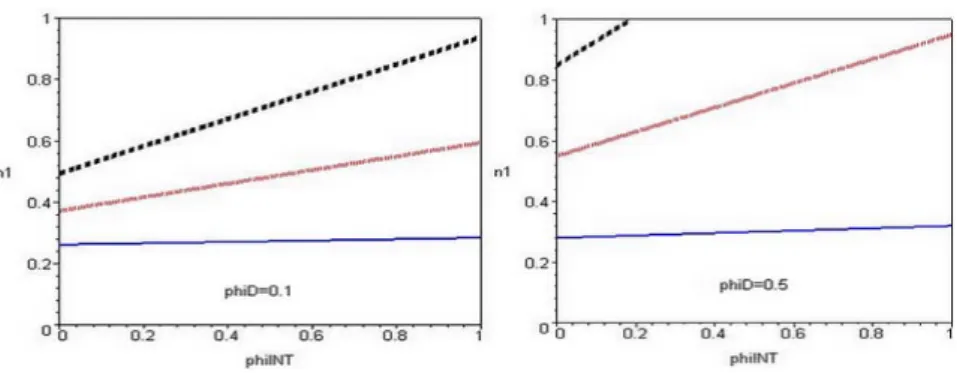
All these insights can be checked in figure 2 where we have plotted the location function for two values of the DTC and three values of region 1’s ex-penditures21. Recall that by hypothesis n1 can not be greater than one-half,

such that all points above n1 = 0.5 are economically irrelevant and n1 just

equals 1/2. We see for instance that when the gap between the two regions is wide (ie, E1 À E3), all northern firms are located in region 1, whatever the

1 9_{We note that, inserting}

c

n1 in the profit-gap, we check that it equals 0, as it is supposed

to, in a long-run equilibrium.

2 0_{Harris[1954] (a geographer) was the first to talk about market potential. His idea was}

that firms tended to locate at places where transport costs related to both inputs (supply) and outputs (demand) were minimal (of course, the size of the local demand and local supply matters in this respect): those places were said to have a high parket potential. Since, lots of papers have been published on this topic; we think that Head&Mayer[2003] is the most influential in this respect, as it tries to clearly define once and for all this concept, and how it is to be applied in economic geography models.

2 1_E

1= 0.26for the solid lines, E1 = 0.35for the small dash lines, and E1 = 0.45for the

Figure 2: The Location Function

value of international transport costs. This effect is magnified when the DTC decrease as shown by the rightmost graph where all lines are translated upward, and where we see that even for a lower expenditure gap between region 1 and region 3 (ie, the small dash line), all firms tend to agglomerate in region 1.

2.3.2 What is Really Going On?

Two thoughts experiments In order to understand the results of the pre-vious section, we need to take a step back and study the profit functions, and in particular the profit gap between region 1 and region 3 (the analysis is sym-metrical for region 2 and 4). If this gap is positive, it is easy to see that firms from region 3 will have an incentive to move. Thus, our aim is to study how the profit gap changes when φI varies22.

To this end, we will attempt two experiments that will help bolster intuition, and shall allow us to isolate the different forces in action. That is, we first evaluate the derivative given that the two regions have the same exogenous number of firms23_{(i.e., n}

1= n3), and then, when the two regions spend the same

amount (i.e., E1= E3). This should allow us to isolate a ”market-access effect”

(ie, firms tend to locate where demand is large) and a ”market-crowding effect” (ie, firms tend to shy away from locations with a huge number of competitors). We recall that after some simplifications, π1−π3= (1−φD)(E1/∆1−E3/∆3).

Thus, in the first case, we have: ∂(π1− π3) ∂φ_I ¯ ¯ ¯ ¯ n1=n3 = −1₂ ∙ (1 − φD) (E1− E3) n1(1 + φD) +12φI ¸ (14)

2 2_{Note that in this section we do not intend to carry an analysis of the stability of symmetric}

interior equilibrium, which would be the case if we were to differentiate the profit gap around the long run equilibrium with respect to n1,for a given value of the transport costs. What we

will do is evaluate the profit gap when we approach a long run equilibrium (for a given value of φI) and the value of φIchanges.

2 3_{As the two regions are not of equal size, the fact that n}

1= n3 must imply that the profit

gap is not equal to zero (and is indeed positive) and we are not at a long run equilibrium. Anyway, we can still study whether the profit gap grows when the international transport costs decrease and at what conditions.

What kind of insights does it give us? First, we see that, for a given egal-itarian allocation of firms in the North, the profit gap variation with respect to the international transport costs decreases with the difference in expenditure E1−E3. In fact, equation (14) enables us to answer the following simple question

: starting from a situation where firms are equally distributed between the two northern regions, which one would benefit more from a further decrease in inter-national transport costs? Here, we see that firms in region 3 will benefit more from an increase in φ_I. The reason is straightforward: the increase in demand from the foreign country associated with a decrease in international transport costs is relatively more beneficial for a small market than for a large one. We note that when the domestic transport costs are negligible (i.e., φ_D = 1), the variation is equal to zero, which is indeed quite logical as it means that the domestic distribution of firms does not matter.

The solution to our second case is: ∂(π1− π3) ∂φ_I ¯ ¯ ¯ ¯ E1=E3 = E1(1 − φD) (∆1− ∆3)(∆1+ ∆3) (∆1∆3)2 (15) Here, the process of signing the derivative is slightly more complicated as it depends on the sign of ∆1− ∆3. Nevertheless, recalling that ∆1 ≡ s1n +

φ_Ds3_n+ φ_Is∗_n and ∆3≡ s3n+ φDs1n+ φIs∗n we find quite easily that ∆1− ∆3=

(1 − φD)(n1− n3).Therefore, the more firms there are in region 1, the more

the profit gap increases with φ_I. This stems from the increase in international competition induced by a rise in φ_I which is more detrimental to a firm located in the region where there are fewer firms as local competition is less strong. In fact, the increase in international competition tends to decrease profits in both regions, but region 3’s profits shrink more as a consequence.

The General case This is how it works: even if the market is larger in re-gion 1, some firms will remain in rere-gion 3 as competition there is less fierce; moreover, an increase in φ_I tends to intensify competition in both regions but this effect is relatively stronger in the region where there are less firms. Mean-while, it becomes less and less important to be located near the large domestic market due to the mere presence of region 2 and 4: indeed, as we have already observed, the bigger international market (region 2 and 4 combined) becomes more easily reachable since international transport costs decrease; one could say that the relative size of region 1’s market shrinks as ITC decreases. This works against agglomeration in region 1. All in all, the increase in competition seems predominant24_{, which explains why firms in region 3 have an incentive to move.}

Conclusion 1 Provided that regions are not totally symmetric, a decrease in international transport costs creates incentives for firms to agglomerate in one region, the rich one, this effect being more important when domestic transport costs are high.

2.4

Welfare

2.4.1 Some useful distinctions

At a very basic level, two notions are generally associated with welfare issues, those of equity and efficiency. When we want to study equity in the context of a geography model, we have to answer the simple question "Are there any losers from agglomeration? Do some regions benefit more than others from a decrease in transport costs?" Efficiency relates to the overall gain (or loss) that comes with agglomeration: that is, even though some people might loose, if the region/nation/world as a whole is better off with more agglomeration, agglom-eration is said to be efficient. This distinction between equity and efficiency is easily understood using the metaphor of a pie, as Baldwin et al [2003] have done:

"If we picture the welfare of the economy as a pie, equity is about the relative size of the slices that go to different interest groups, irrespective of the overall size of the pie. Efficiency, in contrast, is about the overall size of the pie."

In this part, we will focus mainly on equity questions. Our motivation stems from our thinking that, although it is satisfying to know from a theoretical point of view that a country as a whole will benefit from agglomeration, and that a well-done transfer will enhance everyone’s welfare, from a practical point of view, we all know that such transfers are hard to implement. For instance, it might be difficult for a french farmer to understand that more globalization which will lead to his cutting prices will benefit France as a whole, and as such will also be good for him. In our model, the question we want to answer is simple: we have seen that a greater integration between countries leads to agglomeration of firms in a single region, but who benefits from these relocations?

2.4.2 Equity

First, we introduce our metric for welfare: Wk= ln Vk, Vk=

Ek

P , P ≡ G

α_p1−α

T (16)

where Vk is the indirect utility function associated with the preferences of

equation (2)25 _{of a consumer living in region k, W}

k is a concave transformation

of Vk, and P is the prefect price index. In this section, we will approximate

2 5_{Recall that the indirect utility function is defined as the maximum utility that can be}

attained given money income and goods prices. An easy way to check that V is the indirect utility function associated with (2) is to use Roy’s identity to obtain the demand functions associated with V. For the traditionnal good it yields:

−xT= µ dV dpT ¶ / µ dV dE ¶ = −E(1 − α)p −α T Gα_(p−α T )2 / 1 Gα_p1−α T

welfare with the indirect utility function W. Our goal will be to evaluate this W for four kinds of agents26 _{(as usual, we focus our study on northern agents):}

the capital owners of region 1 and 3, and the workers of region 1 and 3. As we have assumed that the initial equal distribution of firms between countries remain the same over time, this is all we have to take into account to study equity in this model. Thus, recalling that each worker provide one unit of labor (and does not hold any capital) and each capital owner own one unit of capital (and does not work), using (5), (6), (7), (8), and (9) yields:

W₁K= ln µ b ∆−a₁ ¶ , W₃K = ln µ b ∆−a₃ ¶ , W₁L= ln µ 1 ∆−a₁ ¶ , W₃L= ln µ 1 ∆−a₃ ¶

where a ≡ σα−1, W1K is the welfare of a region 1’s capital owner, W1L is

the welfare of a region 1’s worker. Recall that ∆1 ≡ s1n+ φDs3n+ φIs∗n and

∆3≡ s3n+ φDs1n+ φIs∗n.

First, we observe that the nominal incomes of each group (the E’s) are in-dependent of both transport costs and localisation of firms. This is a direct consequence of (10), and the fact that, at equilibrium, the reward to capital everywhere equals the world average, that is bEW_/KW_{. Thus, the welfare of}

the different agents only depends on what we could call their "local" price index, that is, the total price they pay to get all the different varieties of industrial good they wish to consume, which represent, in other words, their cost-of-living. As usual in this litterature, these price indexes decrease with the number of lo-cal firms. Thus, we see readily that if region 1 start attracting firms (i.e., ds1

n = −ds3n > 0 ), ∆1 grows while ∆3 decreases (because φD < 1): the real

incomes in region 1 increase while they decrease in region 3. On the contrary, nothing happens between inhabitants of the same region. In the context of our model, we can draw the following conclusion:

Conclusion 2 A decrease of the international transport costs which fosters ag-glomeration in the initially richer region, improves the welfare of this region’s habitants to the detriment of those living in the poorer region. We also note that workers and capital owners of a given region are affected in the same way by movements of firms, such that there is no conflict of interests within a region. Finally, for a given level of transport costs, the spatial distribution of firms is obviously Pareto-efficient since it is not possible to improve region 3’s welfare (by arbitrarily moving firms between regions) without reducing region 1’s.

= −(1 − α)E pT

where we see that we have the CT of equation (3).

2 6_{It is easier to differentiate between workers and capital owners if we assume that workers}

don’t own capital, and that capital owners don’t work. Thus, if each worker provides one unit of labor and each capital owner owns one unit of capital, there will be Kkcapital owners and

3

The 2x4 Model with Comparative Advantages

3.1

The differences

The only two differences between the model in this section and the previous one are that (i) regions are now completely identical in terms of endowments, and (ii) that regions 1 and 2 will have an inherent advantage in the production of industrial goods. We will assume that they, as in the previous section, need only one unit of capital to produce one unit of good, while the other regions need η (> 1) units of capital to produce one unit. For the sake of simplicity, we assume that the η is the same in region 3 and region 4. This "comparative disadvantage" is solely in the fixed cost (i.e., capital) for analytical convenience. This type of modelization was first used in Forslid&Wooton[2003] where they added comparative advantages to the CP model.

Why use comparative advantages? The reason is simple: we think that in the context of a 25-country EU, the comparative advantages some new mem-bers have might offset other advantages like, say, a better market-access, a high-skilled workforce...which the western European countries possess. Indeed, Slovakia, with a population of 5.5m (low local demand ) is becoming one of the car manufacturing centres of Europe (as the investments there of Volkswagen, Hyundai or Peugeot have shown) thanks to relatively low wages (comparative advantage)27. Moreover, the fear of firms moving from high-wages western Eu-rope countries towards low-wages central EuEu-rope countries, is becoming more and more visible, as one can conclude just listening to politicians all over Eu-rope, with the word "delocalisation" being all the rage28_{. Anyway, note that}

in our setting, a region in each country will benefit from a comparative ad-vantage, so that our model do not exactly depict the EU25. Nevertheless, we could stretch the model a bit and assume that the two countries are in fact two regions, say, western Europe and central Europe; and that the two regions (1 and 3/ 2 and 4) are in fact two countries inside those regions, with one having some comparative advantage29_.

In the new setting, the total cost equation becomes: CTk

i = πk+ wLamxi for k = 1, 2 (17)

CT_ij = ηπj+ wLamxi for j = 3, 4

Thus, we note readily that now Kw_{will be different from n}W_{. Indeed, since}

in some regions more than one unit of capital is needed to produce one unit of industrial good, it is straightforward that there will be less firms than units of capital. The new relation is:

2 7_{Admittedly, Slovakia has many other assets which attract investors, like low corporate}

taxes, and a workforce that, even though not as well educated as a western one (and even this is debatable!), is still more skilled than, say, a malaysian one.

2 8_{For instance, Laurent Fabius says about the EU ’s draft constitution: "it has grave}

defects, notably on social issues" as for him "the most important questions for Europe are jobs and délocalisation " (The Economist, September 18th)

2 9_{We need to assume that in both western Europe and central Europe there are differences}

Kw= n1+ n2+

1

η(n3+ n4) (18)

The new no-arbitrage condition, i.e., such that capital movements cease, is: π1= π2=

1 ηπ3=

1

ηπ4 (19)

We see that the profits in region 3 and 4 have to be greater than those in region 1 and 2 for capital movements to cease, because of the comparative disadvantage of these regions: indeed, the same amount of capital will produce fewer units of good in region 3 and 4, such that profit (ie, the return of one unit of capital) there has to be higher in order to attract capital.

3.2

The long-run equilibrium

Once again, we wil focus on the analysis of the northern regions, that is we will study the profit-gap π1−1_ηπ3 . Straightforward but tedious calculations yield

the new location function: n1= 1 4+ (η − 1)£(1 + φ_D)2_{+ 4φ} I(φD+ φI+ 1) ¤ 4(η + 1)(1 − φD)2 (20) which, clearly, depends on η. We see readily that whenever η = 1, n1equals 1

4, that is, firms are equally distributed between regions in a country. This result

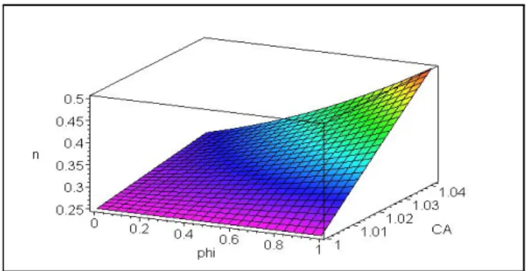
is not surprising if we recall that, in this section, we have assumed that regions are similar in terms of endowments, in such a way that the only thing that makes them different is the comparative advantage. If η = 1, all regions are indeed completely identical, and firms have no incentives to relocate in any one of them in particular. This is shown in figure 3, where we have plotted equation (20) for different values of η the comparative advantage (CA), the ITC, and holding the DTC constant (i.e., φ_D = 1/2). We see that as long as η = 1, the share of firms in region 1 remains at 1

4 for every value of the ITC. Then, whenever η

becomes greater than 1, region 1 starts attracting firms. We also observe that the concentration of firms grows with both φ_I and the comparative advantage. Note that in all graphics, n1 ’s upper level is 1/2; this is so because we have

assumed in the spirit of symmetry that the division of firms between countries would remain constant over time, such that each country own one-half of the total number of firms.

In figure 4, we have plotted the location function, once again holding the DTC constant (ie, φ_D= 1/2), but for only three values of η: the solid line is for η = 1.01, the small dash line for η = 1.03, and the heavy dash one for η = 1.05. We see that, the bigger the comparative advantage of region 1 (i.e., the greater η is), the "faster" agglomeration in region 1 will occur: indeed, for the highest value of η (i.e., the heavy dash line) full agglomeration in region 1 (i.e., n1 = 1/2) occurs for a ITC slightly higher than 0.8, while for lower values of

Figure 3: Region 1’s share of firms as a function of ITC and CA

Figure 4: Region 1’s share of firms as a function of ITC

the comparative advantage of region 1, the more attractive this region becomes, and the more firms want to locate there (for a given value of the transport costs).

To study analytically the impact of transport costs over the location of firms, we will differentiate the location function with respect to φ_I :

∂n1 ∂φ_I = (η − 1)Φ 4 [(η + 1)(1 − φD)2] 2 where Φ ≡ (1 + φD+ 2φI).

We find that it is positive, provided that (i) η is greater than 1 (ie, the country has a comparative advantage in the production of the industrial good) and (ii), that φ_D is less than 1 (ie, domestic trade incurs transport costs). This result confirms what we had found in figure 3.

Conclusion 3 We can conclude that, when international transport costs de-crease, firms tend to agglomerate in the region having a comparative advantage in the production of industrial goods, everything else being equal.

4

Conclusion

In this paper we have extended the FC model to a 2 country-4 region setting in order to study regional inequality. The greatest asset of the FC model is its simplicity that allows for almost limitless modifications to the basic framework, while still remaining analytically tractable. Our first results are consistent with "stylized fact 2" stated in the introduction. Indeed, we found that a decrease in international transport costs fosters the polarisation of manufacturing activ-ities inside countries, as long as regions within countries are differentiated in some way, be it larger demand or comparative advantages (this certainly can be generalized to any kind of advantage). Moreover, we have also found that in the context of a growing international integration, low domestic transport costs tend to intensify agglomeration thus leading to more regional discrepancies. Fi-nally, we have seen that such a decrease of international transport costs enhance the welfare of factor owners in the rich region to the detriment of those living in the poor region.

The present model can be improved and/or prolonged in at least three ways: 1. First, a common comment was that we should allow for migration of labour (at least between regions), which seems a more realistic hypothesis. Above all as migration is one of the most sensitive issue of the European enlarge-ment: most EU15 countries fear that they are going to be "overrun" by an invasion of eastern and central Europe workers that will steal local jobs. Nevertheless, the tricky part of allowing, in the model, people to move, is that, when we allow for regional movements of labour, its distribution within countries becomes endogenous, increasing the number of endoge-nous variables30. Moreover, as we noted in the text, this hypothesis might, after all, be a better guess of what will happen: indeed, a note published by Oxford University Press for the European Commission has calculated that 250 000 to 450 000 workers will travel from East to West in the next two years, and that this figure will fall to 100 000-200 000 migrants a year, after that; thus, ten years from now, between 1.5 to 4 millions of people will have migrated from eastern and central Europe, which amount to less than 5% of the EU15 total population. It should be noted that regional migration is also pretty much retarded in Europe31_.

2. We could introduce some dynamics within the model: indeed, even though studying industrial agglomeration/des-agglomeration might be used as a first approximation of convergence/divergence, it is self-evident that it is rather limited, and that, ideally, a stricter definition of convergence

3 0_{However, we can try to guess what would happen if we allow for labor movements.}

Basi-cally, if labour becomes "interregionaly footloose" it seems that, everything else being equal, it would reinforce the agglomeration forces: indeed, workers will have a tendency to locate in the region with more firms as the price index there is lower (because there are more varieties that are available without having to pay the transport costs).

3 1_{"...even internal migration within the EU member states has been low by world standard,}

should be used. Using a growth engine will also allow us to study both the balanced growth path of the two economies, and maybe, the transitional dynamics. Moreover, in this paper convergence between countries is more of an assumption than a result, as countries start and remain identical. An ideal model should be able to obtain both convergence between countries and divergence between regions at the same time.

3. Finally, the four-regions setting is ideal for studying the question of the "Border-effect"32_{. Indeed, a common empirical puzzle in economic}

geog-raphy is the presence of a strong border effect in Europe, even though the growing integration between european countries should have reduced its strenght. Nevertheless, a possible theoretical explanation of this border-effect is that, as firms tend to agglomerate in a particular region inside a country (when international transport costs decrease), trade in the man-ufactured good is supposed to increase mechanically between the two re-gions, as one is specializing in the manufactured good, while the other specializes in the traditional good. Thus, the border-effect would be a by-product of a growing integration, since this integration creates regional specializations, as we have shown in our model. One also has to consider that the region that specializes in the T-good might prefer to buy the M-good in the other country when ITC decreases. Clearly, there are two opposite effects. A way to find out which effect dominates in our setting, is to compare the market shares of region 1’s firms, in region 3 and region 4 as ITC decreases. Unfortunately, in this model, the result is not satis-factory since we find that there’s no border effect: when countries become more integrated, trade in the manufactured good increases more between them than between two regions of the same country33_{. Clearly, this}

ques-tion has to be studied in a slightly different setting, where internal trade increases more than external trade when the ITC decreases.

5

References

BALDWIN R.E., FORSLID R., MARTIN P., OTTAVIANO G.I.P., ROBERT-NICOUD F. (2003), Public Policies and Economic Geography, Princeton Uni-versity Press

BEHRENS, K., GAIGNE, C., OTTAVIANO G.I.P, THISSE, J-F. (2003), " Interregional and International Trade: Seventy Years after Ohlin", CEPR Dis-cussion Paper, n◦4065

3 2_{McCallum[1995] was the first to identify this so-called border effect: he found that,}

every-thing else being equal (ie, equal sizes and distance), two regions would trade more if they were not separated by a national border. Moreover, other more recent studies such as Nitsch[2000], Head&Mayer[2000]...found this effect to be quite important, and not decreasing over time.

3 3_{We have to compare s}13_{, the market share of a region’s 1 firm in region 3, and s}14_{, the}

market share of a region 1’s firm in region 4. Thus, we find that s13_/s14_{= φ}

D/φI which is

obviously decreasing in φI. It means that when the ITC decreases, firms in region 1 tend to

CANOVA, F. (1999), "Testing for Convergence Clubs in Income per-capita: A Predictive Density Approach", CEPR Discussion Paper n◦ ₂₂₀₁

CROZET, M., KOENIG-SOUBEYRAN, P. (2002), "Trade Liberalization and the Internal Geography of Countries, CREST Discussion Paper N 2002-37 DAVIS, D., WEINSTEIN, D. (1999), ”Economic Geography and Regional Pro-duction Structure: An Empirical Investigation”, European Economic Review, Vol 43(2)

DE LA FUENTE, A., VIVES, X. (1995), “Infrastructure and Education as Instruments of Regional Policy: Evidence from Spain”, Economic Policy, n◦₂₀

EUROPEAN COMMISSION (1996), "Economic Evaluation of the Internal Market, European Economy"

FAGERBERG, J., VERSPAGEN, B., (1996), "Heading for divergence? Re-gional growth in Europe reconsidered", Journal of Common Market Studies, Vol 34

FORSLID R. (1999), “Agglomeration with human and physical capital”, CEPR Discussion Paper, n◦2102

FORSLID R.,OTTAVIANO G.I.P. (2003), "An analytically solvable CP model", Journal of Economic Geography,Vol 3(3)

FORSLID R., WOOTON I., (2003), "Comparative Advantage and the Location of Production", Review of International Economics, Vol 11(4)

GIANNETTI, M. (2002), "The Effect of Integration on Regional Disparities: Convergence, Divergence or Both?", European Economic Review, Vol 46 HARRIS, C. (1954), “The market as a factor in the localization of industry in the United States”, Annals of the Association of American Geographers, Vol 64

HEAD, K., MAYER T., (2000), “Non-Europe : The Magnitude and Causes of Market Fragmentation in Europe”, Weltwirtschaftliches Archiv, Vol 136(2) HEAD, K., MAYER T., (2003), " The Empirics of Agglomeration and Trade", Handbook of Regional and Urban Economics, Vol 4, forthcoming

HEAD, K., MAYER, T., RIES, J. (2002), ”On the Pervasiveness of the Home Market Effect”, Economica, Vol 11(3)

KRUGMAN, P., LIVAS, E. (1996), “Trade Policy and Third World Metropo-lis”, Journal of Development Economics, Vol 9 (1)

McCALLUM, J. (1995), "National Borders Matter: Canada-US Regional Trade Patterns”, American Economic Review, Vol 85

MAGRINI, S. (1999) " The evolution of income disparities among the regions of the European Union", Regional Science and Urban Economics, Vol 29

MARTIN, P., ROGERS, C.A. (1995), ” Industrial location and Public In-frastructure”, Journal of International Economics, Vol 39(3)

MAURSETH, P.B. (2001), "Convergence, Geography and Technology", Struc-tural Change and Economic Dynamic, Vol 12(3)

MICHELIS, L., YIN, L., ZESTOS, G.K. (2003), "Economic Convergence in the European Union", Journal of Economic Integration, Vol 18(1)

MIDELFART-KNARVIK, K.H., OVERMAN, H. (2002), "Delocation and European Integration: Is Structural Spending Justified?", Economic Policy, Vol 35(17)

MONTFORT, P., NICOLINI, R. (2000), "Regional Convergence and Inter-national Integration", Journal of Urban Economics, Vol 48(2)

NEVEN, D.J., GOUYETTE, C. (1995), "Regional Convergence in the Euro-pean Community", Journal of Common Market Studies, n◦₃₃

NITSCH, V. (2000), “National Borders and International Trade: evidence from the European Union”, Canadian Journal of Economics, Vol 22(4)

OTTAVIANO, G.I.P. (2001), "Monopolistic Competition, Trade, and En-dogenous Spatial Fluctuations, Regional Science and Urban Economics, Vol 31 OTTAVIANO, G.I.P., TABUCHI, T., THISSE, J-F, (2002), "Agglomeration and trade revisited, International Economic Review, Vol 43

OTTAVIANO, G.I.P., THISSE, J-F.(2002), "Integration, Agglomeration and the Political Economics of Factor Mobility", Journal of Public Economics, Vol 83(3)

PACI, R., PIGLIARU, P.(1999), "Technological Catch-up and Regional Con-vergence in Europe", University di Cagliary, CRENOS, Mimeo

PUGA, D. (1999), “The Rise and Fall of Regional Inequalities”, European Economic Review, n◦₄₃₍₂₎

PUGA, D. (2001), "European Regional Policies in Light of Recent Location Theories", CEPR Discussion Papers n◦ ₂₇₆₇

QUAH, D. (1996), " Empirics for Economic Growth and Convergence", Euro-pean economic Review, n◦₄₀

REDDING, VENABLES, A.J. (2003), " Economic geography and International Inequality", Journal of International Economics, Vol 62(1)

SALA-I-MARTIN, X. (1996), "The Classical Approach to Convergence Analy-sis", The Economic Journal, n◦₁₀₆

SHIELDS, G.M., SHIELDS, M.P. (1989), "The Emergence of Migration Theory and a Suggested New Direction", Journal of Economic Surveys, n◦₃

VENABLES, A.J., WINTERS, L.A. (2003), " Economic Integration in the Americas: European Perspectives", forthcoming

6

APPENDIX

A stability analysis of the Core-in-North case

In this appendix we will study the Core-in North equilibrium (i.e., π1 =

π3 > π2 = π4 and s2n = s4n = 0: all firms are located in the North, but

there are firms in both northern regions). What we want to know is the set of conditions such that the CIN equilibrium is stable. Thus, we will find the value of the international transport costs where the qualitative properties of the CIN equilibrium will change. As we said in the text, the local stability analysis is done evaluating the profit gap π1− π4 (or π1− π2 for that matter) around the

CIN equilibrium and checking its sign: for the CIN equilibrium to be stable, this profit gap has to be non-negative, otherwise firms would have incentives to relocate in regions 2 or 4. The problem here is that we do not know the internal

distribution of firms in the North, we only know that all firms are located in the North (that is, n1+ n3= 1). The solution consists in a two-step procedure :

(i) first, we find a location function derived from the π1= π3 condition (which

implies that there are firms in both northern regions) which will give us the value of n1as a function of the parameters and then, (ii) we plug this value into

the profit gap π1− π4 and evaluate it around the CIN equilibrium. On to the

first part: we solve π1− π3= 0 recalling that E1+ E3= 1/2 by hypothesis, and

that in the CIN equilibrium n1+ n3= 1 and n2= n4= 0, which yields:

n1=

2 (E1− φDE3)

1 − φD

≡ fn1 (A4)

Note that it does not depend on the international transport costs, which seems logical since the distribution of firms within the North does not depend on the strength of the ITC.

Then, we have: π1− π4 ¯ ¯ ¯ ¯n2=n4=0 n1+n3=1 = E1(1 − φI )φ_I+ (φ_{I− φD})∆1 φ_I∆1 (A5) +E3 (φ_{D− φI})φ_I+ (φ_{I − 1)∆}3 φ_I∆3

Here we need to find the critical value of the ITC such that the profit-gap is nil. First, we plug_fn1in ∆1 and ∆3and find:

π1− π4=

2φ_D(φ_DE1− φI) + 2φI(φI− 1) + φD− 2E1+ 1

2φ_I(φ_D+ 1) (A6)

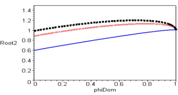
Solving this expression for φ_I yields two critical values of the ITC: φCRIT_I =1 2 µ φ_{D+ 1 ±}q¡φ2_{D− 1}¢_{(1 − 4E}1) ¶ (A7) First, note that the two roots are both equal to 1 when interregional trade is costless (i.e., φ_D = 1): it means the sustain point is φS_I = 1, that is the CIN equilibrium is never stable, provided international trade is not totally free. Then, when interegional trade incurs a transport cost, the two critical values obviously diverge. The one that substracts the radical is always less than one (because it is monotonically increasing in φ_Dand as we have seen above, when φD= 1, the two roots are equal to one) while the one that adds the radical is

sometimes higher than one, as one can see in figure 534. What configurations of parameters yield a root higher than one? Basically, we see from the equation of the two roots that for a given φ_D, the higher the expenditures in region 1 are, the higher the radical is. Moreover, for smaller values of E1, the root can also be

higher than one if φ_D is high. Indeed, for any given value of the expenditures,

3 4_{The heavy dash line is for E}

1= 0.49, the small dash for E1= 0.4, and the solid one for

Figure 5: The second root as a function of the DTC

it is possible to find the value of the DTC such that the second root just equals one:

φ_D= 1 − 2E1 E1

(A8)

Thus, we see that when E1 is small, φDhas to be rather high for the second

root to exceed one.

What does it tell us? Recall that by definition the φ’s are only defined from zero to one, such that any combinations of parameters that would give a value of φ greater than one is economically irrelevant. Nevertheless, for some values of the parameters, both roots are smaller than one which means that the sign of the profit gap changes twice when the ITC decreases, as figure 635 _shows,

while if the second root exceeds one, the profit gap is first negative, and then always positive (see the dash curves in the rightmost graph in figure 6 for an illustration).

What insights did we get? First, we have seen that when DTC are not too low and region 1 is a lot "richer" than region 3 (i.e., E1 is high), the profit gap

remains positive after the ITC have decreased since the second root exceeds one. Moreover, the first root decreases with E1. To sum up, when the gap

between region 1 and region 3 is wide, the CIN structure is "more" stable, in the sense that it becomes stable for higher values of the international transport costs (i.e., small φI) and remain stable hereafter. For lower values of E1, the

profit gap becomes positive for higher values of φI and then, for even higher

values becomes negative. Thus, when (i) the ITC are very low, (ii) the gap between region 1 and region 3 is smaller than in the previous case, and (iii) the DTC are rather high, the CIN structure is not stable (see the heavy dash curves in figure 6, and above all the one in the leftmost graph). It seems to

3 5_{The small dash curve is for E}

1= 0.45, the heavy dash one for E1= 0.35,and the solid

Figure 6:

imply that the advantage of being located in the North becomes less and less important as ITC diminish. For even lower values of E1 (like the solid curves in

figure 6), the profit gap is almost always negative. Finally, note that the CIN structure becomes "less" (ie, for fewer values of the ITC) stable as the DTC decreases. Overall, the decrease of domestic transport costs is a force working against agglomeration in a single country (recall that the decrease of domestic transport is a force working for agglomeration in a single region).

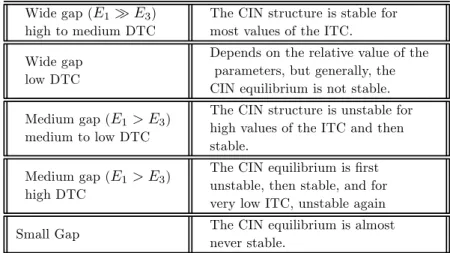
A short summary of our findings:

Wide gap (E1À E3)

high to medium DTC

The CIN structure is stable for most values of the ITC. Wide gap

low DTC

Depends on the relative value of the parameters, but generally, the CIN equilibrium is not stable. Medium gap (E1> E3)

medium to low DTC

The CIN structure is unstable for high values of the ITC and then stable.

Medium gap (E1> E3)

high DTC

The CIN equilibrium is first unstable, then stable, and for very low ITC, unstable again Small Gap The CIN equilibrium is almost

never stable.

We have found a striking result: the more the riches are concentrated in a single northern region, the more likely a concentration of firms in the North is (i.e., it is stable for more values of the ITC), provided DTC are not too low. Basically, when the two northern regions are pretty close in terms of size, firms have incentives to remain in both countries, while if one region is far richer

than the other, firms are better off agglomerating in a single country. There is clearly a link between concentration at the regional level and concentration at the international level. Overall, the decrease of ITC is a force in favor of agglomeration in a single country, provided domestic transport costs are not too high.