The impact of climate change and human management on the water cycle of China : dealing with uncertainties

(1)

HAL Id: tel-02388501

https://pastel.archives-ouvertes.fr/tel-02388501

Submitted on 2 Dec 2019

HAL is a multi-disciplinary open access archive for the deposit and dissemination of sci-entific research documents, whether they are pub-lished or not. The documents may come from teaching and research institutions in France or abroad, or from public or private research centers.

L’archive ouverte pluridisciplinaire HAL, est destinée au dépôt et à la diffusion de documents scientifiques de niveau recherche, publiés ou non, émanant des établissements d’enseignement et de recherche français ou étrangers, des laboratoires publics ou privés.

on the water cycle of China : dealing with uncertainties

Xudong Zhou

To cite this version:

Xudong Zhou. The impact of climate change and human management on the water cycle of China : dealing with uncertainties. Meteorology. Université Paris-Saclay, 2018. English. �NNT : 2018SACLX097�. �tel-02388501�

(2)

Th

`ese

de

doctor

at

NNT

:2018SA

CLX097

The Impact of Climate Change and

Human Management on the Water Cycle

of China: Dealing with Uncertainties

Thèse de doctorat de l’Université Paris-Saclay préparée à l’Ecole Polytechnique Ecole doctorale n 579 Sciences mécaniques et énergétiques, matériaux et géosciences (SMEMAG)

Spécialité de doctorat : météorologie, océanographie, physique de l’environnement

Thèse présentée et soutenue à Palaiseau, le 4 Décembre 2018, par

MONSIEUR

XUDONG

ZHOU

Composition du Jury : M. Laurent LI

Directeur de recherche, Laboratoire de Météorologie Dynamique Président M. Aaron BOONE

Charg´e de recherche, Centre National de Recherches

M´et´eorologiques Rapporteur

Mme. Eleanor BLYTH

Directeur de recherche, Centre for Ecology & Hydrology Rapportrice M. Philippe CIAIS

Directeur de recherche, Laboratoire des Sciences du Climat et de

l’Environnement Examinateur

M. Jan POLCHER

Directeur de recherche, Laboratoire de Météorologie Dynamique Directeur de thèse M. Tao YANG

(3)

(4)

Résumé en français

Introduction

Les changements climatiques et les interventions humaines ont modifié le cycle de l’eau terrestre au cours des dernières décennies. La modélisation du débit des rivières, qui mesure avec précision l’état du système hydrologique, est un moyen pratique de quantifier et de comprendre les impacts du climat et des activités humaines. Cependant, de nombreuses sources d’incertitude peuvent affecter l’exactitude de l’estimation du débit. Ces sources incluent les incertitudes dans les variables atmosphériques qui sont utilisées pour forcer les modèles, les incertitudes dans le modèle lui-même (structure et paramètres du modèle) et les incertitudes dans la formulation des activités humaines. Sur la base de la revue des études en cours présentées dans le chapitre1, cette thèse a pour objectifs de 1) quantifier et comparer les incertitudes de différentes sources, 2) d’attribuer le biais du modèle à différentes sources d’incertitudes et 3) d’évaluer l’impact des activités humaines dans le contexte d’autres sources d’incertitudes. De nouvelles approches sont développées pour ces objectifs et toutes les applications sont centrées sur les régions chinoises.

Quantification de l’incertitude avec une nouvelle approche

l’incertitude existe dans les variables atmosphériques (p.e., les précipitations) et peut être estimée à parmi plusieurs jeux de données. Le chapitre2 introduit une nouvelle approche tridimensionnelle de partitionnement de la variance, particulièrement adaptée à la quantification de l’incertitude entre plusieurs jeux de données comportant des variations temporelles et spatiales. Les multiples jeux de données qui nous intéressent sont organisés selon trois dimensions (c’est-à-dire le temps, l’espace et l’ensemble) illustrées dans la Figure1.

L’incertitude Ueest estimée sous la forme du rapport de la racine carrée de la variance à la dimension d’ensemble (Ve) et de la moyenne du grand ensemble de tous les jeux de données (µ).

Ue =pVe/µ (1)

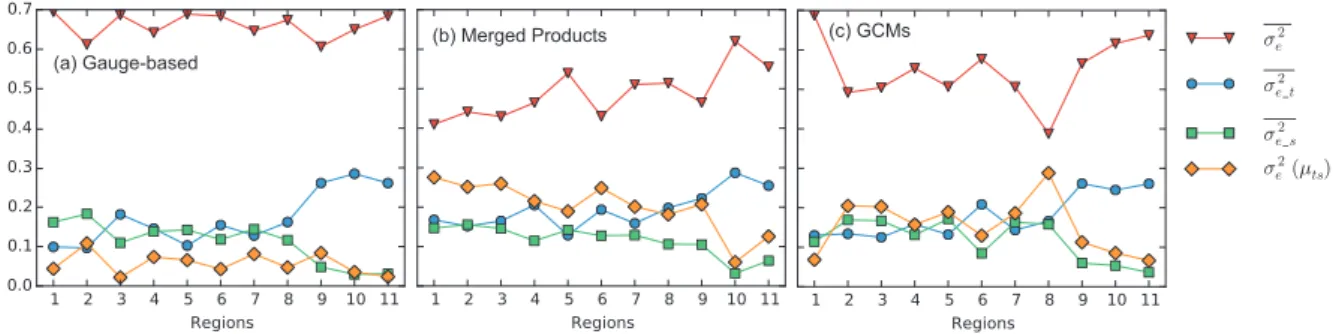
La variance d’ensemble (Ve) est une intégration de la moyenne de quatre types de variances de données d’origine ( 2

e), la moyenne temporelle ( e_t2 ), la moyenne spatiale ( e_s2 ) et la grande moyenne ( 2 e(µts)). V_e = mn(l 1) 3(mnl 1)[ 2 e_t+ e_s2 2 + e2+ e2(µts)] (2)

m, n, lsont les tailles en trois dimensions, respectivement. Parmi les différentes variances, les 2

e_tet e_s2 sont des mesures couramment utilisées pour estimer l’incertitude dans diverses études, tandis que les variations temporelles ou spatiales doivent être éliminée en raison de la limite de leur algorithme pour estimer ces deux métriques.

(5)

Ensemble: d [1:l] Time: t [1:m] Time variance (Vt ) Enseble variance (Ve ) Space variance (Vs ) μ_s μ_e σ2 t σ2 s σ2 e μ_se μ_ts σ2 et σ2 se σ2 ts σ2 t(μse) σ2 s(μet) σ2 e(μts) σ2 t_s σ2 s_t σ2 e_t σ2 t_e σ2 s_e σ2 e_s μ σ2

F 1 – L’illustration de l’approche de partitionnement de variance en trois dimensions. Le jeu de données d’origine est organisé en trois dimensions : temps, espace et ensemble (la zone bleue). Les détails des dénotations et des formulations peuvent être trouvés dans le Chapitre2, Figure2.1et AnnexeA.

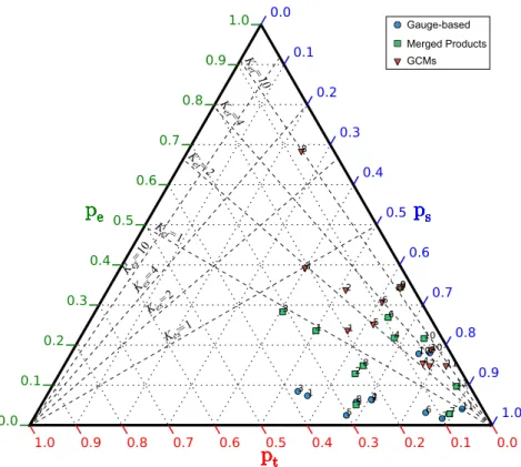
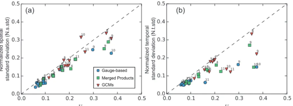
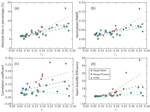
La mise en œuvre de la nouvelle estimation de l’incertitude (Ue) pour différents produits de précipitation (Table2.1) montre que Ue est généralement plus grand que les deux mesures classiques 2

e_t et e_s2 (rapport de la racine carrée de leurs valeurs à la moyenne, Figure 2) car temporelle et spatiale les variations sont prises en compte dans l’estimation Ue. Les différents produits de précipitation basés sur des pluviomètres ont le moins d’incertitude car ils se basent sur des observations similaires et les méthodes d’interpolation n’entraînent pas de grande différence entre les jeux de données. Les ensembles de données de précipitations combinées avec les observations, les satellites, les prévisions et les données de réanalyse ont un Uemodéré, car ils reposent sur différentes sources de produits, tandis que les observations contraindront les valeurs proches du système réel. Le plus grand Uese trouve parmi les modèles de circulation générale (GCMs) car il n’y a pas de contrainte sur la variabilité temporelle dans les modèles de GCMs. Les variations du modèle et les différences dans les conditions initiales entraîneront de grandes différences dans la production finale des précipitations dans le GCMs. Ueest plus grand pour les grandes régions (région 9,10,11) que pour les petites régions en raison des plus fortes hétérogénéités spatiales.

Attribuer le biais de décharge à différentes sources d’incertitude

Différentes incertitudes peuvent survenir et interagir les unes avec les autres, ce qui rend difficile la détermination de la source l’incertitude principle et de comparer les sources d’incertitudes. Le chapitre3introduit un cadre ORCHIDEE-Budyko, qui permet d’attribuer le biais de la décharge modélisée par un modèle de surface terrestre à différentes sources (p.e., variables atmosphériques, structures de modèle) avec l’hypothèse de Budyko.

Le concept de base peut être expliqué à l’aide de l’illustration de la Figure 3. Nous dispersons les points qui représentent les relations entre l’évapotranspiration potentielle

(6)

Gauge-based Merged Products GCMs (a) (b) Normalized spatial standard deviation (N.s.std) Normalized temporal standard deviation (N.t.std)

F 2 – La relation entre Ueet (a) l’écart type spatial normalisé - N.s.std ( q

2

e_t/µ) et (b) le temps normalisé écart type - N.t.std (q 2

e_s/µ). Les valeurs proches des symboles indiquent différentes régions spécifiées dans la Figure2.2.

annuelle modélisée et l’évapotranspiration réelle modélisée avec la précipitation (points rouges). Le point A représente l’état moyen de la simulation du modèle et la courbe représente la relation de Budyko estimée suivant l’état modélisé. Comme il existe des incertitudes dans de nombreuses sources, le débit estimé de la rivière est différent des observations. Les points B, C, D représentent trois états supposés différents qui pourraient modifier les simulations du modèle pour correspondre aux observations des débits en modifiant uniquement le P (point B) ou le PET (point C) ou le ET (point D). La différence entre leurs nouvelles valeurs de P, PET, ET aux nouveaux états (B, C, D) peut être expliquée par les différentes incertitudes. Les variations de P et de PET sont attribuées à l’incertitude des variables atmosphériques et les variations de ET sont attribuées a la structure et aux parameters du modèle. Cependant, cette approche ne donne qu’un éventail des incertitudes maximal. L’état naturel réel se situe très probablement dans la zone ombrée de la Figure3. La possibilité de sources d’incertitude différentes peut être évaluée en consultant d’autres études dans des régions présentant des caractéristiques climatiques ou géophysiques similaires, mais pour lesquelles les données sont moins incertaines.

Budyko curve - model Budyko curve - shifted Modeled annual values Modeled representative state

(P, PET, ET) PET/P ET/P State-Assumption 1 (P’, PET, ET’) State-Assumption 2 (P, PET’, ET’) State-Assumption 3 (P, PET,ET’)

F 3 – L’illustration du cadre ORCHIDEE-Budyko.

La mise en œuvre dans le bassin versant source de la rivière Tarim (Yarkand par exemple) est présentée dans la table1. La décharge observée pour le Yarkand est 140,4 mm/an alors qu’ORCHIDEE la sous-estime à 59,0 mm/an. Il existe trois options différentes (B, C et D)

(7)

mm/an à 225,0 mm/an (point C) ou nous diminuons le ET de 43,2% de 188,3 mm/an à 106,9 mm/an.

T 1 – Les valeurs moyennes annuelles pour différentes composantes eau-énergie (P, ET_{, PET ; unités en mm/an) et leurs relations (P - ET, PET/P et ET/P) pour les trois} sous-bassins amont. Yarkand est pris comme exemple et la table complète se trouve dans la Table3.5. Les scénarios correspondent aux diagnostics du modèle actuel (A) et des trois hypothèses de biais énumérées ci-dessus de B à D. Les valeurs en gras sont les principaux facteurs modifiés au sein des trois composantes du cycle eau-énergie. Le rapport de variation (C.R.) indique le rapport entre la valeur de changement et la valeur d’origine (unité en %). Alors que la plage de biais (B.R.) indique le biais entre valeurs actuelles et ce qu’elles devraient être (unité en %).

P PET ET P ET PET/P ET/P Facteur C.R. B.R.

Yarkand

A 247,3 1240,4 188,3 59,0 5,02 0,76 - -

-B 435,4 1240,4 294,9 140,5 2,85 0,68 P 76,1 -43,2

C 247,3 225,0 106,9 140,4 0,91 0,43 PET -81,9 451,2

D 247,3 1240,4 106,9 140,4 5,02 0,43 ET -43,2 76,1

En faisant référence à d’autres études sur des régions présentant des caractéristiques climatiques ou géophysiques similaires, nous évaluons la possibilité de différentes sources d’incertitude. Les résultats montrent que dans le bassin versant de Yarkand, l’apport d’eau dans le système (P) est certainement sous-estimé car il devrait y avoir un ratio plus élevé de fonte des glaciers et une tendance plus élevée du débit compte tenu de sa fraction de surface de glacier élevée. Cependant, le biais en P n’est pas le seul facteur en cause, puisque PET est excessivement élevé (1240,4 mm/an) pour cette région montagneuse, car les régions proches ne disposent que de 580 à 720 mm/an de PET. PET n’est également pas le seul facteur d’incertitude, car le chargement de PET uniquement réduira le rapport PET/P (indice d’aridité) à 0,91, ce qui est peu probable pour une région aux précipitations limitées. La surestimation de ET est possible, mais ce n’est pas le seul facteur à prendre en compte, car seule la modification de ET augmentera le rapport PET/P à 5,02, ce qui n’est pas une valeur réaliste pour le captage en rivière. Les explications complètes se trouvent dans les sections 3.4.3et la Table3.6.

Activités humaines et comparaisons des grandeurs

Les activités humaines sont des facteurs importants qui modifient le cycle naturel de l’eau et le débit des rivières. Le chapitre4passe en revue les études associées aux différents types d’activités humaines et à leurs impacts sur le débit des rivières en termes de débit totale et extrêmes. L’impact de l’activité humaine sur le débit des rivières a été généralisé à la Figure4.

Différentes utilisations des sols et régulations des barrages ont lieu à différents endroits et leurs impacts sur les régimes de débits des rivières peuvent entraîner des variations dan les amplitudes et phases. La modification des forêts (déforestation et reboisement) modifie à la fois la valeur totale de l’apport en eau et les débits extrêmes des rivières (pics de crue et faible débit). L’expansion de la zone urbaine augmente le pic d’inondation et réduit le temps de résidence de l’eau dans la zone. Il augmente également la valeur totale de l’apport en eau en raison de la moindre évaporation. L’eau utilisée à des fins domestiques et industrielles modifie

(8)

Amount of river discharge E xt re m e s of ri ve r d isch a rg e Urbaniz ation Indus. & Domes. Dams Increase Increase Decrease Decrease

F 4 – Le résumé illustratif de l’impact de l’utilisation des terres et des eaux ainsi que des barrages sur le débit des rivières.

peu le débit du fleuve (2,0 % en moyenne pour la Chine), tandis que la consommation d’eau agricole diminue le rendement total en eau de 7,4 % (en moyenne pour la Chine) pour les cultures. La consommation d’eau a très peu d’impact sur les débits extrêmes, tandis que la régulation du barrage modifie principalement le cycle inter-annuel en diminuant les fortes crues et en augmentant les débits faibles. La quantité totale d’eau diminue légèrement à cause des barrages en raison de l’augmentation de la surface de l’eau et de l’utilisation de l’eau pour l’agriculture essentiellement.

Le chapitre4passe également en revue les approches utilisées pour quantifier les impacts humains sur le débit des rivières. Ils sont classés en deux groupes différents selon que l’impact humain est estimé directement par les modèles. Les concepts de base, les modèles exacts, les études de cas, les avantages et les inconvénients des deux groupes d’approche sont détaillés dans le chapitre4.

Le chapitre4 évalue également l’impact de l’utilisation de l’eau par l’homme et de la régulation de l’eau en comparant les débits observés des cours d’eau et des cours d’eau naturalisés à 84 stations sur les fleuves de Chine. Trois mesures différentes sont utilisées pour quantifier les changements sous forme de valeurs moyennes µ représentant le débit annuel total du fleuve et deux mesures de mise en phase, la période de concentration Cpreprésentant la période au cours de laquelle le débit de la rivière est le plus élevé et le degré de concentration Cd représentant le magnitude de décharge dans la période du débit maximal (équation4.13 -4.18). Les résultats montrent que l’impact humain est faible dans le sud de la Chine, tandis qu’il est important dans les régions du nord où l’agriculture est très développée. Les principales caractéristiques de l’impact humain sont les suivantes : 1) le débit total de la rivière diminue ( µ < 0, 2) la période de concentration est retardée ( Cp > 0) car la consommation d’eau est concentrée au printemps et au début de l’été lorsque le débit naturel du fleuve n’a pas atteint son niveau le plus élevé. En période d’inondation, lorsque le débit de la rivière est élevé, les besoins en eau de l’homme (impact humain) deviennent moins importants. 3) Le degré de concentration diminue ( Cd < 0), indiquant que le débit de la rivière est distribué de manière

(9)

Les changements dans les métriques du débit de la rivière dus aux interventions humaines sont comparés à l’incertitude du débit natural modélisé (Figure5). La différence entre des simulations forcées par différentes entrées atmosphérique est due à la limitation de nos connaissances sur les variables naturelles, y compris le forçage et les modèles. Les métriques (µ, Cp ou Cd) sont estimées séparément pour des simulations de décharge conduites avec différentes entrées de forçage (WFDEI_CMA, E2O, ITPCAS, WFDEI_CRU). L’incertitude de la décharge modélisée est évaluée comme étant la différence des métriques ( µ, Cpou Cd) pour un forçage donné (E2O, ITPCAS, WFDEI_CRU) par rapport à forçage de référence (WFDEI_CMA). Les comparaisons pour chaque bassin versant est tracée dans la Figure5.

DL-River discharge (b) (c) (a) SH-Δμ SH-ΔCp SH-ΔCd Songhua R. Hai R. Huai R. Pearl R. Yellow R. Yangtze R. WFDEI_CRU E2O ITPCAS 13.5% 27.4% 34.5%

F 5 – Comparaison des impacts humains et de l’incertitude de la simulation de décharge entraînée par différents intrants de forçage.

Les résultats montrent que la différence entre le débit simulé du fleuve, qui est causé par la limitation des connaissances, est plus grande que le décalage du débit du fleuve dû aux interventions humaines dans la plupart des régions en termes de débit moyen ( µ) (Figure5). Cela signifie que le choix d’un forçage différent entraînera une différence de simulation de décharge plus grande que ce qui peut être détecté comme étant l’impact humain. L’estimation de l’impact humain n’est donc pas crédible dans ce cas. Cependant, l’écart de différence dû à la limitation des connaissances est moins important pour les métriques de phasage que la période de concentration ( Cp) et la degee de concentration ( Cd) que pour les valeurs moyennes degré de concentration. La proportion de captages qui remplissaient la condition, à savoir que la différence due à la limitation des connaissances est moins importante que le changement dû à l’impact humain, est plus élevée pour Cpet Cd. Par conséquent, Cpet Cd sont de meilleurs indicateurs que les moyens pour attribuer l’impact humain. Nous appliquons le même processus aux précipitations et à l’évapotranspiration potentielle dans le chapitre4, et les résultats montrent que nous avons déjà une bonne connaissance de la phase des variables de forçage, mais la capacité du modèle à estimer la phase de débit du fleuve doit encore être améliorée.

Conclusions et perspectives

En conclusion, cette thèse porte principalement sur les incertitudes inhérentes à l’évaluation de l’impact du changement climatique et à la gestion humaine sur le cycle de l’eau. Les incertitudes des variables atmosphériques sont estimées avec une nouvelle approche de partitionnement de variance en trois dimensions. Le biais de décharge entre les simulations et les observations est attribué aux incertitudes du forçage et à celles dues aux modèles. Les

(10)

résultats montrent que les incertitudes dans le forçage sont grandes et plus grandes que celles pouvant être causées par les modèles. L’impact humain évalué par la différence entre le débit observé et le débit naturalisé est inférieur aux incertitudes liées au débit modélisé pour la plupart des régions, en particulier dans le sud de la Chine. Cela indique que l’attribution des changements à l’impact humain n’est pas possible pour ces régions. Alors que, pour la zone d’irrigation intensive (p.e., le nord de la Chine, le centre du Yangtsé), l’impact humain est plus important que les incertitudes, ce qui permet de pensez que les changements pourront être attribués aux activitités humaines.

La perspective de cette thèse appelle des améliorations dans les modèles pour qu’ils traitent mieux des activités humaines. Les interactions des interventions humaines avec le système d’eau naturel doivent être considérées à une résolution plus élevée de la modélisation de la surface terrestre. L’analyse des incertitudes est également nécessaire pour l’évaluation de l’impact de l’homme, en particulier dans les régions fortement incertaines (p.e., forçage de variables ou de modèles). Ces développement proposées pour les modèles de surface seront discutées plus en détail dans ma thèse chinoise qui sera publiée dans six mois.

(11)

(12)

Remerciements

I would like first to thank Jan Polcher, my thesis supervisor at Laboratoire de Météorologie Dynamique, Paris. I still remember you showed me around the lab on the first day I arrived. It seems you opened a door for me to a new world. You not only helped me a lot on the thesis but also taught me how to do scientific works in a right way. I thank you for your supervision during the last three years.

I would also like to thank Tao Yang, my Chinese supervisor at Hohai University, Nanjing. It is now the eighth year since I knew you. I very appreciate it that you guided me in the first steps of doing research and you brought me a lot of new ideas which broaden my knowledge. I also thank you for your support when I am doing the thesis in France.

I would also like to thank Philippe Ciais and Laurent Li to be members of my thesis committee, and for their wise advice during last three years. I thank Eleanor Blyth and Aaron Boone for agreeing to be the reviewers of my manuscript and for their detailed comments and pertinent remarks.

I would also like to thank Thi Kim ngan Ho, Audrey Lemarechal and Xavier Quidelleur for their help in the administration work for my studying in France. I thank Isabelle Ricordel, Philippe Drobinski and other administrative and computer staff at LMD who allowed me to do my research in good conditions.

I would also like to thank all the researchers who have helped to progress my thesis. Particularly, I would also like to Patrice, Matthieu, Zun, Shilong, Xuhui, Shuai, Xiaoming, Feng, Shushi.

I am very grateful to the members of our small working team. Thanks especially to Trung, for your help on the coding and discussion on my questions. And thanks for sharing your stories during our coffee time. Thanks to Fuxing for our discussion on the modelling and after-work entertainment.

Thanks to the people who shared the same office: Adrien, Thibault, Eivind and Marwa. Thanks also to all those who have made my staying colourful: Rodrigo, Bastien, Nicolas, Aurore, Leo, Artemis, Olivier, Marko, Ariel, Sara, Laurent ... Thanks especially to Adrien, Rodrigo, Patrick and those lovely people I could not tell the names for the pleasant time on the basketball court.

My thanks also go to all my friends who lived in the fifth floor of Collège Néerlandais: Akhil, Hassan, Ali, Fouad, Julia, Katia, Martin, Monica, Nana, Selma, Seray ... Thanks especially to Akhil and Hassan for their accompanying and our interesting philosophical discussions. Thanks to Yohanes (John) who is the first foreign friend of mine. Thanks to Shuowen, Yanting, Jia, Xin and other Chinese students for their help when we were together in France.

I would also like to thank the team members in China: Pengfei, Xiaoyan, Zhenya, Tong, Xin, Peng, Xiaoli, Chao... and the classmates Zhenchen, Dongjing, Huating, Wei ... Many

(13)

The most significant thanks are given to my family members. Thanks to my parents and my grandparents for your love and support in my life. Special thanks to my girlfriend Huidi. Thank you for your accompanying in the last six and a half years. Thanks for your understanding and encouragement in my PhD period. Hope we can find our ways and forge ahead together.

Finally, I would like to thank all those I have met and whom I have not had a chance to say thank you. Thank you, et Merci!

(14)

1

Introduction

1.4 Plan of the thesis . . . . 15 In this chapter, we present the general background which calls for the further understanding of the topic of uncertainties in climate change and human impacts (section1.1). Focused on the China regions, we review the associated studies that show the current state of our understanding and the technologies have reached (section1.2). The scientific questions and the objectives of this thesis are concluded based on the reviewed studies (section1.3). The thesis structure is introduced in the end (section1.4).

(17)

1.1 Scientific context

The global water cycle is undergoing changes in the context of climate change (Gates et al. 2000; Huntington2006; Gerten et al.2008). While, the regional signal is more significant as different changes in the trends of river discharge and the occurrence of hydrological extremes (e.g., floods, droughts) are found in different regions (Gates et al.2000; Wisser et al.2010; Immerzeel et al.2010). The spatial variations of hydrological changes are observed in China as well. The river discharge in the Yellow River was sharply decreased in the last century especially in the 1990s as the zero-flow days reached up to 226 days in 1997 (Xu2004). The occurrence of floods and droughts in the Yangtze River basin are found increasing especially after 2000 (Chen et al.2014). These regional changes will exert direct influence on local social development and thus require equal attention at a regional scale to that of global scale.

The changes in regional hydrological regimes are a combined result of climate change and human activities (Wang et al. 2010b; Yang et al. 2010; Zhang et al. 2010; Yang et al. 2012a; Zhao et al.2014; Lu et al.2015; Jiang and Wang2016). The changes in climate (e.g., precipitation, temperature) vary across space regarding its trend and its magnitude by the influence of various regional climate systems (IPCC2013). Moreover, the human activities take place with spatiotemporal variations, and the interactions between human and nature are complex in terms of the physics and the consequences (Piao et al.2010; Nazemi and Wheater 2015a; Nazemi and Wheater 2015b; Wada et al. 2017). It calls for further investigation on how the climate and human are affecting the water cycle as well as the corresponding methodologies for the purpose.

Modeling is a practical way to hindcast the water cycle in the historical period or the future (Döll et al. 2009; Hanasaki et al.2010; Guimberteau et al. 2012b). Modeling also provides estimates of variables that are difficult to measure but can improve the understanding of water processes (e.g., the soil moisture, the actual evapotranspiration, Potter et al.2005; Weiß and Menzel2008). It makes the simulations possible under different scenarios which help to attribute the hydrological changes to different reasons (Chen et al. 2009; Schewe et al.2014). However, there are many uncertainties which can affect the accuracy of model simulations and result in different conclusions (Beven and Freer2001; Refsgaard et al.2006). The uncertainties are either because of the inaccuracy of data measurements or due to the deficiency of the model ability to represent natural physical processes (Moradkhani et al.2005; Thyer et al.2009; Montanari et al.2009). These uncertainties are in many cases interrelated with each other (Renard et al.2010). Therefore, recognizing the uncertainties and their impact on the water cycle, exploring and disentangling the interactions between uncertainties are essential in the hydrological modeling.

Humans are playing a role in changing the hydrology for the benefit of social development (Haddeland et al.2006; Wada et al.2017). However, human interference varies in time and space, and it is especially strong in the area where the agriculture widely distributes and when society is rapidly developing (Haddeland et al. 2006). China is one of the countries that rely highly on agriculture, and it experienced rapid increases in both its population and its economy in the last few decades (Liu et al.2008; Piao et al.2010). China also spans a large area with different climate types and topography (Wang et al.2017a). Thus the water cycle in

(18)

1.2. Literature review 3 China and its responses to the climate and human activities have their different characteristics which need an overall review. The methodologies for estimating the hydrological responses and their peculiarities should be summarized as well for better understanding and utilization of the methodologies.

In this chapter, the current studies on the spatial variations in hydrological changes and the association with climate change and human impacts are reviewed. The descriptions of different uncertainties in hydrological modeling, as well as the current quantification methods of the uncertainties, are also collected and discussed in this chapter. The scientific questions that remain to be investigated are summarized based on the current studies.

1.2 Literature review

1.2.1 Climate change and hydrological impacts in China

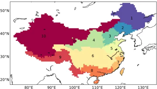
China spans a broad range of longitude and latitude and has complex topographic conditions and climatic features (Wang et al.2017a). Changes in the climate over China in the meantime have significant spatial variations as the trend in atmospheric variables (e.g., precipitation, temperature) are different at the regional scale (IPCC2013). In a report by China’s National Climate Change Program (CNCCP 2007), it was shown that China observed an average temperature increase of 0.5-0.8o_{C during the past 100 years (1900-2000). There was no} obvious trend of change in annual precipitation, but there exists considerable variation among regions. The decrease in annual precipitation was significant in the northern China, averaging 2.0-4.0 mm/yr while precipitation was increased in the southern China with a rate of 2.0-6.0 mm/yr. The observed river discharge1 measures the responses of the land water system to the changing environment, and it has significant spatial variations similar to that of the precipitation. Zhang et al. (2007) analyzed the gauge discharge records in six large river basins in China (i.e., Hai River, Yellow River, Huai River, Yangtze River, Southeast Rivers and Pearl River, Figure1.1) over period 1950-2004. They concluded that the basins in northern China were experiencing significantly declining in discharge during the study period, especially in the 1990s. Among which the Yellow River, Huai River and Hai River are the basins where the discharge changed significantly. While in southern China, the discharge changes were not apparent (e.g., the Yangtze River, the Southeast and Pearl River). The similar changes are also reported in studies by others and on the tributaries of those large river basins with direct gauge observations (Yang et al.2005; Yang et al.2012b; Zhang et al.2013; Zhao et al.2013; Wei et al.2016).

The Yangtze River basin, a representative region of southern China, has the longest river in China with a typical monsoon climate in the middle-low latitudes (Chen et al.2016). The mean temperature is 14.0o_{C and mean precipitation is 1045 mm/yr for the whole Yangtze} River basin for 1955-2011 (Chen et al.2014). The long-term average runoff depth2is 515 mm/yr, accounting for 49.2% of the precipitation (Chen et al.2014). There is a significant

1Discharge: the volumetric flow rate of water that is transported through a given cross-sectional area. 2Runoff depth: the depth to which a watershed (drainage area) would be covered if all of the runoff for a given period of time were uniformly distributed over it.

(19)

Songhua River Liao River Hai River Huai River Yangtze River Pearl River Yellow River Southeast Southwest Northwest

Figure 1.1 – The map of China and the main rivers.

increase in temperature, but no trend is detected for the precipitation for the Yangtze (Chen et al.2014). The change in the observed discharge is not significant at the lower Yangtze river (Zhang et al.2007), while a small but statistically significant increase in discharge and ratio of discharge to precipitation (approximating runoff ratio3) is found upstream of the middle Yangtze River (Chen et al.2014). The increase in the ratio is probably caused by increasing water storage and deforestation, which increases the speed and ratio of surface runoff in the humid Yangtze (Chen et al.2014). For the source catchment of Yangtze, observed discharge decreased from the 1950s to 1980s and then started increasing in the warming environment (Xiong et al.2013). Correlation of the discharge change to the cumulative temperature deficit indicates that the glacier melting may induce the discharge increases in the headwater regions of Yangtze River (Xiong et al.2013). However, the glacier impact is not shown in the middle or lower Yangtze because the proportion of glacier melt becomes small compared to the total runoff in estimations in the lower Yangtze as many river tributaries join the mainstream (Immerzeel et al. 2010). Concerning the seasonal discharge in the middle-low Yangtze, increasing trend (albeit not strong) is detected in the discharge in winter or dry seasons, while the discharge in summer especially in October is decreasing (Chen et al. 2016; Guo et al. 2018). These changes are mainly because of dam constructions and regulations in the Yangtze River basin rather than the climate change as the dams store extra water in flood seasons for reducing the flooding risk and for electricity production, and then it is released in the dry

(20)

1.2. Literature review 5 seasons (Chen et al.2016). For the other rivers in southern China (e.g., Pearl River, rivers in the southeast), the discharge is mainly influenced by precipitation as for the Yangtze, and the variability of observed discharge is always highly correlated to that of precipitation (Li et al. 2016c). The climate change, especially the precipitation changes, will exert direct impacts on the river discharge.

The Yellow River basin, a representative region of the northern basins, has the second longest river in China with semi-arid climate types (Yang et al.2015a). The Yellow River originates from the north Qinghai-Tibet Plateau and the changes of water yield4 in the plateau has significant impacts on the whole Yellow River because the water yield in the upstream accounts for more than 44.8% of that for the whole basin (Wei et al.2016). The Yellow River has experienced a decreasing trend in discharge ranging from 1.0 mm/10a to 16.1 mm/10a at different gauges (Zhao et al.2014). The discharge in the 1990s has declined to 34.2% of that in the 1950s (Wei et al.2016). The zero-flow days occurred in the lower Yellow and increased to the highest (226 days) in 1997 (Xu2004). Although the changes in forcing variables are also significant as the precipitation was decreased by 11.7 mm/10a (1.9-47 mm/10a, Wei et al.2016), human activities are generally regarded as the dominant factor of the discharge reduction with their contribution to the discharge ranging between 55-83% by different estimations (Wang et al.2010b; Yang et al.2010; Zhao et al.2014). Various human activities, especially the water consumption for agricultural use, dam storage and the changes in land use are associated with the discharge reduction in different studies (Wei et al.2016). After 2000, the natural runoff has recovered by 14% in observations, probably because of the combined impacts of precipitation increases (Tang et al.2013), the reforestation in the middle Yellow (Wang et al.2011a), and the improved water management among the dams in the whole river basin (Zhang et al.2009).

With respect to other north river basins such as Songhua River, Liao River, Hai River, Huai River and their tributaries, the observed discharge variations are similar to that of the Yellow River as a significant reduction of discharge is found in the historical period (Zhang et al.2010; Yang et al.2012a; Lu et al.2015; Jiang and Wang2016). Estimated by different approaches with a set of assumptions, human impacts contribute more to the discharge change than that caused by the climate (Gao et al.2013; Chang et al.2016; Jiang and Wang2016). Increasing water consumption is the main factor controling discharge change while water projects (e.g., dams and floodgates) also play a role in the discharge change, such as that in the Yellow River (Zhang et al.2010; Jiang and Wang2016).

Another hotspot region with significant climate change and hydrological alteration is northwest China, where the climate is dry with very little precipitation (Zhou et al.2018). The precipitation change varies spatially and shows a remarkable rise in the North Xinjiang (Kong and Pang2012). Compared to the precipitation, the temperature increase is apparent in northwestern China and over the main rivers of Tarim, Aksu, Heihe River and Urumqi River for instance (Wang et al.2010b; Kong and Pang2012). The snowmelt runoff has apparently increased from 1970 to the present in the upstream of the Heihe River (Wang et al.2010a).

4Water yield: the total amount of water generated by precipitation, snow and glacier melt and groundwater. It consists of surface runoff, subsurface drainage and groundwater recharge. And it equals to the precipitation over a catchment minus the evapotranspiration back to the atmosphere in area free of glaciers.

(21)

The time of snowmelt has shifted ahead and the peak discharge has increased in the snow season (Wang et al.2010a). Temperature increasing also results in accelerating glacier retreat and increases of glacier melt in the high mountains and river basins where the glacier melting is one of the major sources (e.g., Aksu, Yarkand, Kumalak; Wang et al.2012a; Kundzewicz et al.2014; Wang et al.2017a). Kong and Pang (2012) have pointed out that Kumalak river is more sensitive to climate change than Urumqi River as 57% of the discharge in Kumalak is ice-melt while it is only 9% for the Urumqi River. The relation of the temperature and the glacier melt has been proven with a lag time of the discharge phase (1-3 day time lag between the phases of temperature and the observed discharge, Krysanova et al.2015).

Although there have been some studies that discussed the climate change impacts on hydrology in northwestern China as presented above, those studies mainly focused on catchments with a very small areas in the river sources regions. Studies for large basins are still lacking. The situation is attributed to two major reasons. First, the collection of high-quality climatic and hydrological data is challenging for large basins because of the coarse gauge network and high heterogeneity of forcing variables in the mountainous area (Zhou et al. 2018). The hydrological processes in the floodplain and oases are more complicated than that in the headwater catchments. Agricultural activities are mainly concentrated over the lower plains and will significantly change the natural discharge, while the effect of human interference in oases is not well understood or quantified in such dry areas (Tao et al.2011; Zhou et al.2011).

Summary

Climate change and the impacts on the hydrology vary in space in mainland China. For the regions in southern China, the precipitation dominates the changes in river discharge, while there are no significant signals in the trends. For the regions in northern China, precipitation has significantly decreased in the last half-century which is in line with the decreasing discharge. However, because humans highly rely on water resources, the contribution of human activities is always regarded as the main contributor to the discharge decline through simulations. Many studies target on eastern China in terms of climate change and hydrological responses because of sufficient data and relatively simple physical interactions in the regions. While for the regions in northwestern China, the estimation of the discharge response is more complicated owing to data scarcity, large spatial heterogeneity, high uncertainty in glacier changes and intensive human activities. The studies over those regions are therefore fewer and need to be strengthened especially in large basins.

1.2.2 Uncertainties in modeling discharge

The human impact on river discharge is not easily measurable and needs different models for its estimation. However, the quantitative reconstruction of the changes and impact assessment with models may arrive at different conclusions because the used data are not perfectly describing the natural variables and the models are not perfectly describing the physical processes. There are probably large diversities among the results if different inputs,

(22)

1.2. Literature review 7 different methods or different model settings are used for estimations (Refsgaard et al.2006). The possible uncertainty sources that may affect the model results are reviewed in this section. Atmospheric variables

The primary uncertainty comes from the uncertainties in atmospheric variables. For example, as the dominant factor in driving the entire water cycle, the precipitation (P) and its measurement are affected by many factors (e.g., the size and location of the orifice of instruments, the recording errors, Dingman 2015; Mcmillan et al. 2012). Wind may significantly reduce the precipitation catch, especially of small drops and snowflakes (Mueller and Kidder1972; Sevruk1982). The measurement error tends to be larger for low-intensity precipitation because the amount is not enough to trigger a record and the amount is easy to evaporate (Mcmillan et al.2012; Neff1977). The measurement of storm rainfall is also difficult because of the accompanying strong wind. Despite the difficulties of making precipitation measurements, the conversion of precipitation records to what the end users can use introduces other uncertainties. Firstly, because the precipitation records are reported in a fixed short interval (e.g., hourly precipitation, Lenderink and Van Meijgaard2008), while the data to the public are most in daily, the temporal variations of the records at the sub-daily time scale are therefore not able to be captured with public datasets. Secondly, because the precipitation is measured at point gauges, the precipitation between the gauges are estimated with different interpolation methods which are not necessarily able to describe the spatial heterogeneity (Haddeland2002). This situation is more serious in the areas with low-gauge density (e.g., mountainous areas, dry areas) and areas with high heterogeneous precipitation events (e.g., orographic rains and storms, Adam et al.2006; Biemans et al.2009; D’Orgeval and Polcher 2008). The same problems exist for other forcing variables (e.g., wind speed, temperature, radiation, etc., Xu and Luo2015). However, because the spatial variations or the impacts of those variables are not as strong as that of the precipitation, the spatial features of other variables have received less attention.

The uncertainty of the temporal and spatial variations in precipitation are partly solved by improving the interpolation algorithms and by using remote sensing (e.g., satellite, radar radiation, Hong et al.2006; Tapiador et al.2012). Frequency analysis of hourly precipitation over available gauges reveals the temporal patterns of different precipitation types (e.g., hourly distribution of the precipitation) and can be used to interpolate precipitation in time (Lenderink and Van Meijgaard 2008; Shen et al. 2014). Remote sensing can capture the spatial pattern of the potential precipitation (not the actual precipitation reaching the ground) which helps to describe the spatial heterogeneity (Shen et al.2014) of the actual precipitation. Statistical approaches have also been developed for the orographic effects of precipitation in mountains (Adam et al.2006). Precipitation can also be estimated by models (global or regional circulation models). Because these models poorly describe the precipitation spatial patterns, downscaling (e.g., statistically or physical methods) is applied for further usage of the modeled results (Chen et al.2011; Wilby et al.2014; Yang et al.2012b). With the variety of methods, there have been many precipitation datasets that can be used to drive models (Sun et al.2018). The variations of these precipitation datasets will be quantitatively analyzed in

(23)

Chapter2in this thesis.

There are many other atmospheric variables (e.g., temperature, radiation, wind) which have similar temporal and spatial variations. Moreover, uncertainties exist for these variables either through measurement or modeling. Although these variables do not directly affect the water flux (e.g., precipitation) entering the system, they change the thermodynamics which can propagate to the estimation of potential evapotranspiration (PET). The actual evapotranspiration (ET), which denotes the amount of water that leaves land water system and goes back to the atmosphere, will be affected by both the P and PET. PET is not measurable, and there are many kinds of approaches for estimating PET. No matter which approach is used, the uncertainty in the aerodynamic variables will propagate to the final PET estimations, resulting the uncertainties in PET.

Models

The second source of uncertainty is the model diversity in estimating hydrological responses to climate change. A model is an abstraction, simplification and interpretation of the real world (Refsgaard et al.2006). Different researchers have developed different algorithms according to their experiments and understanding of the physical processes. The choice of modules is subjective but limited by data sufficiency (Clark et al.2008). Lumped conceptual models require fewer model inputs than physically based models, and many physical processes in the lumped conceptual models are simplified (e.g., the energy balance, the evaporation estimation, Beven and Freer 2001; Gaume et al. 1998). Moreover, different modules can be selected for the same physical process. For example, both the Green-and-Ampt method and the Horton method estimate the infiltration rates while the Horton equation is empirical (D’Orgeval et al. 2008; Dingman2015; Yu et al. 1999). The methods for estimating the evaporation are even more varied than that for the infiltration (e.g., the Bowen ratio method, the water-balance method, the Dalton equations, McMahon et al.2013). The routing processes are simplified using different methods, and two routing module methods can be chosen depending on whether the model is grid-based (e.g., Total Runoff Integrating Pathways-TRIP, Oki and Sud 1998) or basin-based (e.g., Lohmann routing model, Lohmann et al. 1996). All these methods deal with different processes which differ in terms of their basic assumptions, their required data and thus the scope of their application. They are coded to different modules to integrate with the core model. The diversity of modules will result in differences in model outputs, and this can be regarded as the uncertainty in model structures.

These modules have a certain ability to describe the physics. Thus the selection of the module is not very strict. The improvement of the modules is always on the way to integrate the better understanding of physical processes. For example, the land surface model ORCHIDEE (Organizing Carbon and Hydrology In Dynamic EcosystEms) was initially developed in the 1980s by the Laboratoire de Météorologie Dynamique (IPSL-LMD) (Ducoudré et al.1993). It was directly developed in the GCM but later extracted from the GCM for offline (no coupled) applications (Rosnay and Polcher1998). The model allowed irrigation interactions with soil moisture after 2003 (Rosnay et al. 2003) and interactions with river discharge after 2005 (Ngo-Duc2005). Different infiltration methods were tested in 2008 (D’Orgeval and Polcher

(24)

1.2. Literature review 9 2008). The snow and soil freezing scheme was updated in 2012 (Gouttevin et al.2012). An improved snow scheme was tested in 2013 (Wang et al.2013a). The routing scheme was also updated recently based on high-resolution (1 km) topography information (Nguyen-Quang et al.2018). The continuous exploration of the natural physical phenomena with the support of field experiments and numerical models helps drive the development of models and decreases of the uncertainties due to the deficiency of model structures.

The parameters comprise another model uncertainty source. Most of the model parameters have different values over space while they are taken as constants in models for simplification. For example, in the Variable Infiltration Capacity (VIC) model, the maximum soil depth is taken as 1.9 m in the model in all implementations (Rodell et al.2004). The parameter for the order in variable infiltration equation ranges from 0.2 to 0.6 which is determined by the soil properties, while it is calibrated to be a constant for the entire space (Koch et al.2016). These parameters are in general “free” and can be calibrated to a particular situation when the model is applied (Refsgaard1997). However, the shortcoming is that the uncertainty from other sources (e.g., the model inputs and model structures) are probably attributed to the parameters, and in some cases, the parameters will be out of its reliable range to meet the calibration requirements (Zhou et al.2018). The uncertainty in the parameters is generally reduced by applying field experiments for local studies (El Kateb et al.2013). However, the parameters obtained from field experiments are still difficult to apply at large scales because of the spatial variations (Haddeland2002; Xu and Luo2015) . Uncertainty analysis is instead a more popular way to quantify the impacts of parameters to the model results. With the uncertainty analysis, the consequence of the parameter selection can be measured and then controlled within a limit (Beven and Freer2001). The details of the uncertainty analysis are introduced in section1.2.3in this chapter.

Human activities

The third uncertainty is related to human activities (Krzysztofowicz 2001). Human activities (e.g., irrigation, dam regulation, water consumption) have been incorporated into some models as different modules (Hanasaki et al.2006; Haddeland et al.2006; Hanasaki et al. 2010; Guimberteau et al.2012b). Compared to the natural processes, the parameterisation of human activities is more subjective and lacks information. Moreover, there are differences between the real actions and set modules which have been written in models. For example, although the regulation rules for any dams, canal gates and pumps have been set for different occasions, there is a deviation of the real operations from the standard rules because the participation of experts (Ehsani et al.2016; Nazemi and Wheater2015a; Nazemi and Wheater 2015b). The actual decisions will, to some degree, deviate from what is built in models. These difficulties make the parameterisation hard to correctly represent the human interventions to the natural water cycle.

The uncertainty can also result from unanticipated changes in nature, human goals, interests, activities, demands and impacts especially for future projections (Krzysztofowicz 2001). Concerning human interference with nature, we consider the human impacts to be stable or with a consistent trend in a short future period. However, for example, China’s reform

(25)

and opening policy has suddenly stimulated the social-economic development as well as the consumption of water and loss of land area for urbanisation (Liu et al.2014a; Liu and Tian 2010). On the contrary, from the end of the 20th century, the “Grain for Green” policy has boosted the increasing of forest area, especially in the hydrological-fragile areas. The shift of trends in forest area has caused opposite impacts (increasing river discharge) on the water sphere (Wang et al.2011a) while negative impacts (decreasing river discharge) are found a few years later which were not considered at the beginning of the afforestation projects (Zhang et al.2016, discussed in Chapter4). There are other human activities (e.g., irrigation, dam construction or removal) can start from a specific time in a region but it is difficult to involve them in a model which is designed decades ago without knowing when, where and how the human activities affect the future.

Summary

In conclusion, there are three major uncertainty sources in hydrological modeling. They are the data uncertainty (also named natural variability or aleatory in the literature), the model uncertainty (also named knowledge uncertainty or epistemic) which includes the uncertainty in model structure and model parameters, and the third uncertainty which results from human interferences. Great efforts (e.g., merged products, improvement in algorithms, experiments) have been done to reduce the uncertainties from the different sources. However, the uncertainties are not and can never be eliminated. Moreover, different uncertainties coexist and also interact in the modeling. There is a necessity to quantify the impact of uncertainty from a single source and separate the impacts from the interaction of multiple sources.

1.2.3 Uncertainty quantification

Uncertainty analysis

The model outputs are subject to imprecision with uncertainty because of the various uncertainty sources introduced above. Uncertainty analysis is a derivation of the probability distribution of the model outputs based on the probabilistic description of model inputs and the models (UNESCO2005). The uncertainty analysis can be an analytical way that involves all the differentiation of model equations and the exact probability distribution of all model inputs and parameters (Pechlivanidis et al.2011). It derives the statistics of model output from the knowledge of statistical properties of the system itself and the input data (Langley2000). However, this approach is strongly limited because of its severe requirements on the data information and model equations (Pechlivanidis et al.2011). To decrease the difficulty, many assumptions on the data properties and statistical models are required to avoid describing the natural variability and model processes in an overly complex manner (e.g., the standard probability distribution of the parameter, rainfall-runoff equations). Because the method is analyzing the full probability distribution of model input, model structures and model results, it is called probabilistic analysis in Montanari et al. (2009). The philosophy is used by Krzysztofowicz (2002) in a Bayesian Forecasting System and by Montanari and Brath (2004) in a meta-Gaussian rainfall-runoff approach. Other methods based on the Bayesian

(26)

1.2. Literature review 11 basis, can also be used as the probabilistic framework (Montanari2007), e.g., particle filters (Moradkhani et al.2005) and Bayesian total error analysis (Thyer et al.2009).

The alternative solution, which is more commonly used, is to use sampling strategies to derive the statistics of model outputs numerically (Montanari2007). Uncertainty is quantified by running the model repeatedly with different sets of parameter values sampled from a given probability distribution (Pechlivanidis et al.2011). Although this approach is computationally expensive, it requires no access to the model equations and avoids simplification of model processes (Pechlivanidis et al.2011). It thus can be integrated with many existing hydrological models (Zadeh2005), e.g., TOPMODEL (Beven and Freer2001), HYMOD (Montanari2005). The sampling method is the basic philosophy of the Generalized Likelihood Uncertainty Estimation (GLUE) (Beven and Freer2001; Beven and Prophecy1993). The Monte Carlo sampling method is always used together with GLUE as it obtains random sampling in the input data space and the system space (Ballio and Guadagnini2004; Kuczera and Parent 1998). It does not necessarily require the knowledge of the probability of the samples, but the model performance will screen the samples with a given criterion to obtain the collection of samples (Beven and Freer2001; Beven and Prophecy1993). With the model results generated by the samples, the statistics (e.g., mean, standard deviation, skewness) and the probability distribution of the model output can be determined. The GLUE-based approaches are limited to the analysis of parameters, and they are not able to deal with the uncertainty in model inputs or model structure (Jacquin and Shamseldin2007). Because the sampling methods does not provide a probabilistic solution to the parameters, they are regarded as the non-probabilistic way which is different from the probabilistic approach introduced in the previous paragraph (Montanari2007).

Sensitivity tests

As mentioned above, the analytical approaches desperately require the knowledge of equations on the system input and model itself (Montanari et al. 2009). The sampling approaches are unable to deal with the uncertainties from model inputs and model structures (UNESCO 2005). The sensitivity analysis is instead the most welcoming approach for assessing the impact of different uncertainty sources. The theory of sensitivity analysis is simple since the model simulations are compared in different states with different model settings of interest (e.g., different forcing inputs, different model structure, different model parameters) while keeping all other model settings as the same (UNESCO2005). The changes in the simulations between different states are regarded as the model sensitivity to the changes in the model settings. Compared to uncertainty analysis, the sensitivity analysis does not need to find and assess all states in the whole feasible spaces, but the users can evaluate any states of interest with very few numbers of model runs compared to the sampling approaches (Tang et al.2007). The sensitivity test is also a simplification of the sampling approach in assessing the parameter impact by giving only a few parameter settings instead of searching for the whole parameter space. The shortcoming for the sensitivity analysis is that it only evaluates the model sensitivity to the given model settings, it cannot show the real probability distribution of the model outputs (UNESCO2005). The given model settings are assumed

(27)

as equally frequent although they are not in reality and some of the model settings may be probably out of the reliable range because of the low requirement to the understanding of the models (Zhou et al.2018).

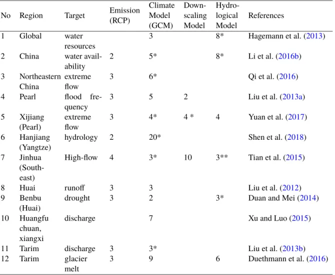
A few implementations of sensitivity tests are listed in Table1.1. These studies span different regions in China and focus on different hydrological patterns (e.g., total water resources, flood and drought, flood frequency, glacier melt). By applying different numbers and types of the uncertainty sources (e.g., emissions, climate models, downscaling models and hydrological models), the sensitivity of the hydrological change to different uncertainty sources are compared in Table 1.1in a very simple way as the hydrological sensitivity to different uncertainty sources are placed in an order. The emissions or the downscaling model will not become the primary factor that changes the final model outputs in most of the cases. Because the climate model determines the driving forcing and the hydrological model determine the physical processes of rainfall-runoff change, both are the major factors that result in significant hydrological changes. It is therefore necessary to further investigate how the climate forcing and the hydrological model change the water cycle.

Summary

In conclusion, knowing the uncertainties from different sources that are further affecting the hydrological model simulations, many studies have focused on different approaches that quantify the hydrological responses to the uncertainties. Uncertainty analysis is frequently used and can be grouped to probabilistic approaches which depend on the full probability distribution, and non-probabilistic approaches which are sampling-based. Sensitivity tests is also an effective way to assess the sensitivity of hydrological responses to different uncertainty sources. Although there have been many implementations related to the uncertainties, research is still needed to deepen the understanding on how the uncertainties, especially from the model inputs and hydrological models, affect the water cycle modeling. The separation of the impact from different sources is not well known. The significance of the human intervention on the water cycle is not clear, especially compared to the uncertainties of the forcing and that of the models.

1.3 Scientific questions and objectives

1.3.1 Scientific questions

By reviewing the above literature, we can draw a few conclusions as below:

• The model input data uncertainty, especially for the precipitation, has been recognized by the science community. Comparisons between different precipitation datasets have been conducted. However, the precipitation comparison among datasets of different types (e.g., gauge-based datasets, merged productions with satellite or radar, pure model datasets) is lacking, and therefore the uncertainties in different data types are not well assessed.

(28)

1.3. Scientific questions and objectives 13

Table 1.1 – Implementations of sensitivity tests among the emissions, climate models, downscaling models and hydrological models.

No Region Target Emission_(RCP) ClimateModel (GCM) Down-scaling Model Hydro-logical Model References 1 Global water

resources 3 8* Hagemann et al. (2013)

2 China water

avail-ability 2 5* 8* Li et al. (2016b)

3 Northeastern

China extremeflow 3 6* Qi et al. (2016)

4 Pearl flood

fre-quency 3 5 2 Liu et al. (2013a)

5 Xijiang

(Pearl) extremeflow 3 4* 4 * 4 Yuan et al. (2017)

6 Hanjiang

(Yangtze) hydrology 2 20* Shen et al. (2018)

7 Jinhua (South-east)

High-flow 4 3* 10 3** Tian et al. (2015)

8 Huai runoff 3 3 Liu et al. (2012)

9 Benbu

(Huai) drought 3 2 3* Duan and Mei (2014)

10 Huangfu chuan, xiangxi

discharge 7 Xu and Luo (2015)

11 Tarim discharge 3 3* Liu et al. (2013b)

12 Tarim glacier

melt 3 9 6 Duethmann et al. (2016)

Note:

The numbers represent the number of different datasets/methods used in the sensitivity test ** represents that the uncertainty source is the primary

* represents that the uncertainty source is the primary (or secondary if there is ** for any source) The study case with no stars means the hydrological sensitivity to all sources is equivalent

(29)

• The hydrological response to different uncertainty sources are investigated using uncertainty or sensitivity analysis in many implementations. However, the separation of impacts from the interactions of different uncertain sources is not well known, and the reliability of the solutions needs further study and discussion.

• Human activity plays an important role in hydrological changes and is a significant uncertainty source. While, when and how much human activities are affecting the water cycle, particularly in China in the past, present and future, need an overall review. The magnitude of the human impact should also be evaluated and compared with the possible uncertainties from other sources.

• Most of the regions in the eastern Chinese mainland have been well investigated in terms of their climatic characteristics and hydrological changes. However, the regions in northwestern China, e.g., the Tarim basin, have received very little attention owing to the difficulties related to data scarcity, hydrological complexity and human activities. Parallel comparisons to the changes over the whole of China should be conducted as well.

The scientific question are therefore posted as “what are the magnitudes of various

uncertainties, their sources, interactions and spatial variations?” To address the

scientific questions, we need to solve the technical problems as 1) to quantify the uncertainty in the model inputs and the models; 2) to explore the interactions of uncertainty from different sources; 3) to compare the magnitude of human impact with our knowledges of natural variables.

1.3.2 Objectives

• Investigate the uncertainties in precipitation, especially for different types of precipitation products; quantify the variances among different precipitation datasets due to the variations between datasets; compare the ensemble variance with the temporal and spatial variances in precipitation patterns; verify the estimated uncertainty with current available technologies.

• Implement a Land Surface Model (ORCHIDEE) in the Tarim basin and estimate the hydrological variables (e.g., discharge, evapotranspiration); analyze the model bias with discharge observations; attributes the bias to uncertainty in model inputs and model structure with a Budyko approach; verify and assess the likehood of different biases. • Review the literature of human activities (e.g., land use, water use, dams) in China in

the past; review the impact (e.g., magnitudes, spatial and temporal patterns) of different human activities on water cycle; review the methods that are used to quantify the impacts of human activities; categorize the methods and compare the peculiarities of the different methods into different categories;

• Qualify the human impact on river discharge and compare the influence due to the limitation of knowledges of natural variables in the forcing and model simulations;

(30)

1.4. Plan of the thesis 15 identify the metrics that can be used to attribute the human impact and identify the catchments where the human impact assessment is easier and with higher confidence.

1.4 Plan of the thesis

CH2. A variance partitioning approach (precipitation uncertainty and ensemble)

• Uncertainties in different precipitation types

• Ensemble analysis and its association with uncertainties

CH3. ORCHIDEE-Budyko framework (uncertainty integration)

CH4. Review and human impact assessment (Human activities and limit of knowledge of nature) • Land Surface Modeling (ORCHIDEE)

• Uncertainty integration with Budyko • Take Tarim basin as the example

• Human activities (land, water use, regulations) • Methods categorization and comparison • Human impacts VS. simulation uncertainties

Input

uncertainty Model uncertainty

Human activities

Figure 1.2 – Flow-chart of the thesis

The structure of the thesis is organized as follows (refer to the illustration in Figure1.2). In Chapter1, the background of the research topics, the related literature, the scientific questions and the objectives of the thesis are introduced.

In Chapter2, a new approach of partitioning the variances in an ensemble analysis is introduced and applied to precipitation datasets. The uncertainties of different types of precipitation are analyzed and associated with the uncertainty estimation with the newly proposed approach.

In Chapter3, a framework named ORCHIDEE-Budyko, which can be used to attribute the model bias in discharge estimation to the uncertainties in model inputs and the model itself, is introduced. The Tarim basin is chosen as the example.

In Chapter4, the recent literature about human activities, particularly in China, is reviewed in terms of understanding the impacts on hydrology. The methods that have been used to estimate the human impacts are also reviewed, and their peculiarities are compared between different approaches. The human impact identified by the difference between observed and naturalized river discharge is compared with the influence due to limitation of our knowledges of natural variables on the forcing variables and estimated water cycle.

(31)

In Chapter5, the conclusions are summarized based on the previous chapters. The key points are further explained and discussed. The perspectives are provided on the basis of the results of the thesis.

(32)