(will be inserted by the editor)
Recursive Petri Nets
Theory and Application to Discrete Event Systems
Serge Haddad1, Denis Poitrenaud2 1
LAMSADE - UMR 7024, Universit´e Paris-Dauphine
Place du Mar´echal De Lattre de Tassigny, 75775 Paris cedex 16 e-mail: Serge.Haddad@lamsade.dauphine.fr
2
LIP6 - UMR 7606, Universit´e Paris VI, Jussieu 4, Place Jussieu, 75252 Paris cedex 05
e-mail: Denis.Poitrenaud@lip6.fr Tel: (33) 1 44 27 71 04
Fax: (33) 1 44 27 87 71
Received: date / Revised version: date
Abstract. In order to design and analyse complex systems, model-ers need formal models with two contradictory requirements: a high expressivity and the decidability of behavioural property checking. Here we present and develop the theory of such a model, the re-cursive Petri nets. First, we show that the mechanisms supported by recursive Petri nets enable to model patterns of discrete event systems related to the dynamic structure of processes. Furthermore, we prove that these patterns cannot be modelled by ordinary Petri nets. Then we study the decidability of some problems: reachability, finiteness and bisimulation. At last, we develop the concept of linear invariants for this kind of nets and we design efficient computations specifically tailored to take advantage of their structure.
Key words. Petri nets – Expressivity – Reachability problem – Bisimulation – Flows computation
1 Introduction
With the increasing complexity of systems, the use of formal models is a requirement for their design and analysis. However, the modeler is faced with a dilemma: he looks for a highly expressive model while
keeping decidable the checking of significant properties. For instance, the inability of automata to represent infinite state systems and the undecidability of termination of systems equivalent to Turing machine exclude them for being practical specification models.
A closer look at the standard patterns of dynamic systems high-lights two modelling needs:
1. A model must handle the concurrent execution of parallel sequen-tial processes.
2. It must also manage the dynamical creation of objects (e.g. re-sources or processes).
We now discuss the advantages and drawbacks of the two most frequently used models: Petri nets (PNs) and process algebras (PA). Whereas modelling concurrent activities is rather straightforward with Petri nets, the management of dynamic objects is limited. In-deed, due to the static structure of the PN, there is no way to keep trace of a synchronisation between two dynamically created processes. With coloured Petri nets [13], such a synchronisation is possible; how-ever, in order to preserve decidability of standard problems, the set of colours (i.e. the number of processes) must be kept finite. From the point of view of verification, the checking of standard properties of PNs and specific properties expressed by event-based linear time logic are decidable problems (see [5] for a survey). Like PNs, process alge-bra are appropriate for the modelling of concurrency. Furthermore, via recursion and parallel composition, they allow synchronisation between dynamically created objects. However, including these two operators leads to a Turing machine equivalent model.
In this paper, we describe a model which we feel is appropriate with respect to both the expressivity and the analysis capabilities: the recursive Petri nets (RPNs) first introduced in [24].
Previous results: We have already defined two versions of RPNs. In the full model, threads which play the token game of a Petri net, can be dynamically created and concurrently executed. In [7, 8], we have studied the expressivity of this model and the checking of some fundamental properties. In particular, we have shown that the RPN model is strictly more expressive than the union of Petri nets and context-free grammars w.r.t. the language point of view. Moreover, we have demonstrated that the reachability problem and some related ones remain decidable for RPNs.
Beside these positive results, we have also shown a negative one in [6]. Whereas the event-based linear time model checking is decid-able for Petri nets, it becomes undeciddecid-able for RPNs. Thus, in [9], we
have introduced a restricted model called sequential RPN (SRPN) for which this problem remains decidable and whose languages fam-ily still strictly includes the union of the Petri nets and context-free languages. Roughly speaking, in an SRPN the executions of threads are nested: only the last created one executes until its termination or the creation of a new thread.
Contributions: The first contribution of this paper is the introduc-tion of an extended version of RPNs including new mechanisms. An RPN has the same structure as an ordinary Petri net except that the transitions are partitioned into two categories : elementary and abstract transitions. The semantics of such a net may be informally explained as follows. In an RPN, there is a dynamical tree of threads (denoting the fatherhood relation) where each thread plays its own token game. A step of an RPN is thus a step of one of its threads. If the thread fires an abstract transition, it consumes the input tokens of the transition and generates a new child which begins its own to-ken game with some starting marking depending on the current state of its father. If the thread reaches a marking belonging to a set of final ones, it aborts its whole descent of threads, produces (in the token game of its father) the output tokens of the abstract transition which gave birth to it and dies. The produced tokens depend on the final marking reached by the thread. In the particular case of the root thread, one obtains an empty tree. If the thread fires an elemen-tary transition, then it updates its current marking using the Petri net firing rule, i.e. it consumes the tokens required by the input arcs and produces the ones specified by the output arcs. Additionally, the firing may abort threads initiated by a previous firing of the current thread.
With respect to the model presented in [8], the current model in-cludes the following additional features: the place capacities, the test arcs, the parametrised initiation and termination of threads and the interrupt capability. We show that the reachability problem remains decidable for this extended version of RPNs. We also prove that the boundedness and the finiteness problems are still decidable. At last, we show how to define and compute some linear invariants which capture relations between a thread and its descendants.
The second contribution of the paper deals with the expressivity of SRPNs. The modelling capabilities of SRPNs can be illustrated in different ways. In this paper, we present the modelling of faults within a system and we demonstrate that an equivalent modelling by an ordinary Petri net is impossible. SRPNs enable also to easily model multi-level executions (e.g. interrupts).
The last contribution is related to bisimulation in the framework of SRPNs. While bisimulation of Petri nets is undecidable, one can check the bisimulation between a Petri net and a finite automaton. We demonstrate that for a subclass of SRPN called restricted SRPN (RSRPN), this problem is still decidable. We emphasise that this restricted model is strictly more expressive than the union of Petri nets and context-free grammars.
Related work: We now relate this model to similar ones. Since the introduction of Petri nets, theoretical works have been developed in order to study the impact of extensions of Petri nets on the analysis capability. For instance, the reachability problem is undecidable for Petri nets with two inhibitor arcs while it becomes decidable with one inhibitor arc or a nested structure of inhibitor arcs (see the unpub-lished manuscript “Reachability in Petri Nets with Inhibitor arcs” by K. Reinhardt reachable at http://www-fs.informatik.uni-tuebingen. de/∼reinhard). The self-modifying nets introduced by R. Valk have
(like Petri nets with inhibitor arcs) the power of Turing machine and thus many properties including reachability are undecidable [26, 27]. Introducing restrictions on self-modifying nets enables to decide some properties [3] (boundedness, coverability, termination, ...) but the reachability remains undecidable. Moreover, these extensions do not offer a practical way to model the dynamic creation of objects.
In order to tackle this problem, A. Kiehn has introduced a model called net systems [14]. Net systems are a set of Petri nets with special transitions whose firing starts a new token game of one of these nets. A call to a Petri net, triggered by such a firing, may return if this net reaches a final marking. All the nets are required to be safe and the constraints associated with the final marking ensure that a net may not return if it has pending calls. It is straightforward to simulate a net system by an RPN. Moreover as the languages of Petri nets are not included in the languages of net systems, the family of net system languages is strictly included in the family of RPN languages.
Another attempt for the introduction of dynamic capability in Petri net is the object Petri nets of R. Valk [28]. In this model, to-kens are themselves Petri nets and the creation of a new process is achieved by the production of a new token net. The hierarchy has a limited depth (two levels) and the synchronisation mechanism can operate only between the upper level and one of the subprocess. It has been demonstrated that reachability is an undecidable problem [15]. A similar model called nested Petri nets has been introduced in [18] presenting the following features: the depth of the hierarchy is un-bounded and vertical and horizontal synchronizations can operate.
Here again, it has been proved that the reachability and boundedness are undecidable even if termination and other standard properties re-main decidable.
Process Algebra Nets (PANs), introduced by R. Mayr [20], are a model of process algebra including the sequential composition opera-tor as well as the parallel one. The left term of any rule of a PAN may use only the parallel composition of variables whereas the right side is a general term. This model includes Petri nets and context-free gram-mars. We have proved [8] that RPNs also include PANs. Whereas we do not know whether the inclusion of the PAN languages by the RPN ones is strict, we emphasise that the main difference between RPNs and this model is the ability to prune subtrees from the extended marking. For instance, this mechanism is indispensable for the mod-elling of plans in multi-agents systems [24]. Moreover, PANs as well as Process Rewrite Systems [21] (a more expressive model) cannot represent a transition system with an infinite in-degree.
Recursive-Parallel Programming Scheme (RPPS) [16] also offers the notion of hierarchical state. Like for RPNs, the synchronisation mechanism is restricted to processes linked by the fatherhood rela-tion. Several interesting problems (e.g. reachability) are decidable for this model. However, it has been shown that the family of languages of Petri nets is not included in the one of RPPS.
Organisation of the paper: We have chosen to introduce first the least expressive model. This progressive presentation will help the reader to get an intuitive view of the model capabilities. In the next section, we define sequential recursive Petri nets. Then, we illustrate its ex-pressive power with the modelling of Discrete Event Systems (DES) patterns. Afterwards, we tackle the bisimulation problem between an SRPN and a finite automaton. The third section is dedicated to the full RPN model: we study its expressivity and we establish the decidability of the reachability and related problems. We conclude this section by defining linear invariants and designing algorithms for their computations.
2 Sequential Recursive Petri Nets 2.1 Definitions
Preliminaries: As our model relies heavily on semilinear sets, we briefly introduce their definition and properties. A semilinear set is a subset of Nd defined as a finite union of linear sets (where
N = {0, 1, . . .} is the set of natural integers and d ∈ N \ {0}). A linear set L is defined by a vector m0and a finite set of vectors {m1, . . . , mk}
such that L = {m | ∃(λ1, . . . , λk) ∈ Nk, m = m0+Pi=1,...,kλi· mi}.
An effective representation is any representation which can be re-duced (by an algorithm) to this standard representation. For instance, any system of linear (in)equalities on the coordinates of vectors is an effective representation. Given an effective representation of semi-linear sets, the following operations are computable: union, intersec-tion, projection and complementation. Furthermore, the membership problem is decidable (see [4] for details).
In our proofs, we implicitly use the effectiveness of the represen-tation, the above operations and the membership test.
We now introduce a particular kind of semilinear sets. Restricted semilinear sets are expressed by a boolean combination of inequalities between a positive weighting of the coordinates of vectors and a natural integer.
Definition 1. A boolean combination φ of inequalities w.r.t. to a fi-nite set of variables {xi}1≤i≤d is recursively defined by:
– either φ =def Σ1≤i≤dai· xi ≤ k where {ai}1≤i≤d and k belong to
N,
– or φ =def φ1∧ φ2 or φ =def φ1∨ φ2 or φ =def ¬φ1 with φ1, φ2 two
boolean combinations of inequalities.
A restricted semilinear set E of Nd is defined by a boolean com-bination of inequalities φ by E = {m | φ({xi ← m(i)}1≤i≤d) is true}
where φ({xi ← m(i)}1≤i≤d) is the boolean value obtained by setting
every variable xi to the constant m(i).
Note that a restricted semilinear set is a semilinear set (see [23]) whereas the converse is not true: x1− x2= 0 defines a semilinear set
which is not a restricted one.
As an ordinary Petri net, a sequential recursive Petri net has places and transitions. The transitions are split into two categories: elemen-tary and abstract transitions.
The semantics of such a net may be informally explained as fol-lows. In an ordinary net, a thread plays the token game by firing a transition and updating the current marking (its internal state). In an SRPN there is a stack of threads (each one with its current marking) where the only active thread is on top of the stack. A step of an SRPN is thus a step of this thread. The enabling rule of the transitions is specified by the backward incidence matrix.
When a thread fires an elementary transition, it consumes the to-kens specified by the backward incidence matrix and produces toto-kens defined by the forward incidence matrix (as in ordinary Petri nets).
When a thread fires an abstract transition, it consumes the tokens specified by the backward incidence matrix and creates a new thread (called its son) put on top of the stack which consequently becomes the active one. Such a thread begins its token game with a starting marking which depends on the fired abstract transition.
A family of effective representations of semilinear sets of final markings is defined in order to describe the termination of the threads. This family is indexed by a finite set whose items are called termi-nation indexes. When a thread reaches a final marking, it terminates its token game (i.e. is popped out of the stack). Then it produces in the token game of its father (the new top of the stack) and for the abstract transition which gave birth to him, the tokens specified by the forward incidence matrix. Unlike in the case of ordinary Petri net, this matrix depends also on the termination index of the semilinear set which the final marking belongs to. Such a firing is called a cut step. When a cut step occurs in a stack reduced to a single thread, one obtains an empty stack.
The next definitions formalise the model of SRPN and its associ-ated states called extended markings.
Definition 2 (Sequential Recursive Petri nets). A sequential recursive Petri net is defined by a tuple N = hP, T, I, W−, W+, Ω, Υ i
where
– P is a finite set of places,
– T is a finite set of transitions such that P ∩ T = ∅,
– A transition of T can be either elementary or abstract. The sets of elementary and abstract transitions are respectively denoted by Tel and Tab,
– I is a finite set of indexes,
– W− is the pre function defined from P × T to N,
– W+ is the post function defined from P × [Tel∪ (Tab× I)] to N,
– Ω is a labelling function from Tab to NP which associates with
each abstract transition an ordinary marking called the starting marking of t,
– Υ is a family indexed by I of effective representations of semilinear sets of final markings.
In the sequel, we reason about two kinds of markings: extended markings and ordinary markings. The former ones are states of SRPN while the latter ones, as in Petri nets, are mappings from P to N
(otherwise stated vectors in NP). When no confusion is possible, we simply call them markings. We introduce a useful notation for such markings: let m ∈ NP and a set P0 ⊆ P , the submarking m|P0 ∈ NP
0
is the restriction of m to P0 (i.e. ∀p ∈ P0, m|P0(p) = m(p)).
Definition 3 (Extended marking). An extended marking tr of a sequential recursive Petri net N = hP, T, I, W−, W+, Ω, Υ i is defined by:
– dtr ∈ N the depth of the extended marking and {1, . . . , dtr} the
set of levels of tr, – mtr1, . . . , mtrd
tr the ordinary markings associated with each level,
– ttr1 , . . . , ttrd
tr−1 a family of abstract transitions indexed by all levels
except the last one.
In order to unify the definitions related to SRPNs and RPNs, we view an extended marking of an SRPN as a tree reduced to a single path where nodes are indexed by levels and labelled by ordinary mark-ings and edges are labelled by abstract transitions. The root of this tree corresponds to the bottom of the stack and the single leaf to its top (for instance, see figure 2).
A marked sequential recursive Petri net (N, tr0) is an SRPN N
together with an initial extended marking tr0.
According to the presentation, the size of the stack corresponding to an extended marking tr is dtr and the ordinary markings
asso-ciated with the threads of the stack are mtr1, . . . , mtrd
tr. The empty
stack (dtr = 0) corresponds to the extended marking without thread
and is denoted by ⊥. Since the effect of cut steps depends on the abstract transition which gave birth to a thread, these transitions (ttr1 , . . . , ttrd
tr−1) are stored in the extended marking.
An elementary step will denote either a transition firing or a cut step. The semantics of SRPN given by the enabling and the firing of steps is summarised in the following definitions.
Definition 4. A transition t is enabled in an extended marking tr (denoted by tr−→) iff ∀p ∈ P, mt trdtr(p) ≥ W−(p, t) and a cut step τi
with i ∈ I is enabled (denoted by tr τi
−→) iff mtrdtr ∈ Υi.
Definition 5. The firing of an enabled elementary step s of an ex-tended marking tr leads to the exex-tended marking tr0 (denoted by tr−→trs 0) depending on the type of s.
– s ∈ Tel – dtr0 = dtr , ∀0 < i < dtr, mtr 0 i = mtri , ttr 0 i = ttri
– ∀p ∈ P, mtrdtr0(p) = mtrdtr(p) − W−(p, s) + W+(p, s) – s ∈ Tab – dtr0 = dtr+ 1 , ∀0 < i < dtr, mtr 0 i = mtri , ttr 0 i = ttri – ∀p ∈ P, mtrd0 tr(p) = m tr dtr(p) − W −(s, t) – ttrd0 tr = s , m tr0 dtr0 = Ω(s) – s = τi – dtr0 = dtr− 1 , ∀0 < j < dtr− 1, mtr 0 j = mtrj , ttr 0 j = ttrj – dtr0 > 0 ⇒ ∀p ∈ P, mtr 0 dtr0(p) = mtrdtr0(p) + W+(p, ttrdtr−1, i)
Let {tri}1≤i≤n be extended markings, {si}1≤i<n be elementary
steps. Then σ = tr1 · s1 · tr2 · s2. . . sn−1· trn is a firing sequence
(denoted by tr1−→trσ n) iff ∀1 ≤ i < n, tri−→trsi i+1. In the sequel
and for sake of simplicity, σ will be often denoted by σ = s1. . . sn−1.
When multiple SRPNs are involved, we denote by tr1−→σ Ntrna firing
sequence σ in an SRPN N . In a marked SRPN (N, tr0), an extended
marking tr is reachable iff there exists a firing sequence tr0−→tr.σ
Definition 6 (Reachability graph). Let (N, tr0) be a marked
se-quential recursive Petri net. Then its reachability graph is defined by hS, A, tr0i where S, the set of nodes, is the set of reachable extended markings of (N, tr0), A ⊆ S × (T ∪ {τi}i∈I) × S is the set of edges
and tr0 ∈ S is the initial node. There is an edge (tr, t, tr0) ∈ A iff
tr−→trt 0.
Remarks: When empty, a set of final markings has no effect on the net behaviour, thus in SRPNs we assume that these sets are non empty (contrary to the RPN case to follow). Furthermore, we allow intersection of such sets to be non empty so that the cut steps may be non deterministic. Morevover, ∀i ∈ I, τi does not belong to T .
2.2 Expressivity of SRPNs
This section illustrates both the syntax and the semantics of SRPN with the help of relevant examples. Furthermore, we simultaneously demonstrate the expressive power of the model and its suitability with respect to standard discrete event system patterns [1].
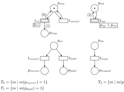
Modelling of interrupts and exceptions: The net of figure 1 illus-trates the characteristic features of SRPNs. The specific features of an SRPN are represented graphically as follow:
– an elementary transition by an ordinary transition (i.e. a single border rectangle),
pex prun pstop tex tcorrect h1i h0i pup+ pint pint tint h2i pex trecover precover tfatal pfatal pup ttreat ptreated Υ0= {m | m(precover) = 1} Υ2= {m | m(ptreated) = 1} Υ1= {m | m(pfatal) = 1}
Fig. 1 an exception and interrupt mechanism
– an abstract transition t by a double border rectangle whose start-ing markstart-ing Ω(t) is specified in a frame by P
p∈PΩ(t)(p) · p, a
symbolic sum with null terms omitted and 1 · p abbreviated to p. When defined and non null, the items W−(p, t) and W+(p, t) in-duce arcs with their corresponding integer labels. These labels are omitted when the valuation is equal to one. There is an arc from an abstract transition t to a place p if at least one item W+(p, t, i) is non null. Such an arc is labelled by the symbolic sumP
i∈IW+(p, t, i)·hii.
As usual, when W+(p, t, i) = 0 the term W+(p, t, i) · hii is omitted and when W+(p, t, i) = 1 this term is abbreviated as hii. Moreover, when for all i the values W+(p, t, i) are equal, the symbolic sum is abbreviated to this common value. We complete the figure with the definitions of the sets {Υi}i∈I. The set I is implicitly given by the
enumeration of these sets.
Figure 1 provides a complete description of an SRPN. Note that contrary to ordinary nets, SRPNs are often disconnected since each connected component may be activated by the firing of different ab-stract transitions. As the initial extended marking is reduced to a single node, we have directly described the ordinary marking asso-ciated with this node by putting token in places. We will follow the same convention in the sequel. The left upper part of the figure mod-els the application level of a processor in an abstract way. The cycle prun, tcorrect, prun represents the correct execution of the current
in-tex pint pfatal tex pint pex tfatal tint prun pup+ pint tint prun ptreated+ pint ttreat prun+ pint tint tex tcorrect τ2 pstop+ pint τ1 tint tint prun pup pup+ pint tint tint tint prun pup pup+ pint ttreat τ2
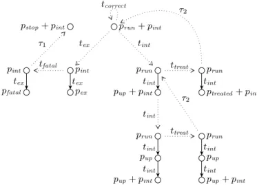
Fig. 2 an extract of the reachability graph of the SRPN of figure 1
struction and the abstract transition tex models a faulty execution of
the instruction yielding a second level with pex marked. In this level,
the system either recovers from the fault (trecover) or detects a fatal
error (tfatal). The sets Υ0and Υ1model these two cases. Depending on
the fault type, when returning to the first level, the process resumes its activity (place prun marked) or stops it (place pstop marked).
The interrupt modelling outlines the capabilities of the SRPN. When the abstract transition tint is fired, the current execution is
interrupted and a second execution level, modelled by a token in pup and pint, is activated. The same construction applies again on
this component net making possible a recursive interrupt process. Some variants are conceivable: the number of execution levels could be bounded with additional places, the interrupt could occur during the exception treatment, etc.
Modularity is a natural feature of SRPNs. Indeed, if the system does not include the interrupt mechanism, the modeler simply deletes the right hand side of the figure.
Figure 2 represents an extract of the reachability graph of the SRPN of figure 1. We graphically represent an extended marking as a path whose nodes correspond to levels and are labelled by the associated ordinary markings and whose edges connect level i to i + 1 and are labelled by ttri for i ∈ {1, . . . , dtr− 1}. Extended markings are
depicted from top to bottom according to their depth. The dashed arcs denote steps between extended markings.
pinit+ pfault pstart tstart trepair prepair pfault pinit tcount pcount Υ0= {m | m(pfault) > 0}
Fig. 3 a basic fault tolerant system
The left part of figure 2 is related to the exception mechanism whereas the right part is devoted to the interrupt occurrences and handling. We just describe a step sequence of the figure. From the initial state, the firing of tex leads to a two level extended marking.
Then the firing of tfatal only changes the ordinary marking of the
active node which now belongs to Υ1. Hence, a cut step τ1 occurs
yielding a single level extended marking where only interrupts may happen.
The example of fig. 1 shows the capability of SRPNs to implicitly keep the context of suspended processes whereas the modelling by Petri nets requires an explicit representation of each context. By use of this capability, we have shown in [8] that SRPNs include the family of algebraic languages. On the other hand, it has been proved that the language of palindromes (a particular algebraic language) cannot be recognised by a labelled Petri net [10]. Thus the language family of SRPNs strictly includes the one of ordinary Petri nets.
Modelling of faults: In order to analyse fault-tolerant systems, the engineer starts from a nominal system and then introduces the fault-ing behaviour as well as the repairfault-ing mechanisms. We limit ourselves to an abstract view of such a system as this pattern may be straight-forwardly generalised. The nominal system infinitely executes instruc-tions (elementary transition tcount). The marking of place pcount
rep-resents the number of instruction executions. The complete SRPN is obtained by adding the left part of the figure 3. Its behaviour can be described as follows. There are only two reachable extended markings reduced to a single node: the initial state (trstart) where a token in
pstart indicates that the system is ready to start and the repairing
state (trrepair) where a token in the place prepair indicates that one
is repairing the system. Starting from the initial state, the abstract transition tstart is fired and the execution of instructions is “played”
a crash occurs, the repairing state is reached. Place pf ault represents
the possibility of a crash. As pf ault is always marked in the correct
system and from the very definition of Υ0, the occurrence of a fault
is always possible. We assume that no crash occurs during the re-pairing stage. With additional places and by modifying Υ0, we could
model more complex fault occurrences (e.g. conditioned by software execution).
The reachable extended markings either consist of a single node or an initial node and its son. However, the number of reachable markings in this latter node is infinite (the place pcountis unbounded).
In other words, the repairing state can be reached from an infinite number of states which means that the transition system associated with an SRPN may have some states with an infinite in-degree. This capability is neither shared by standard Petri nets nor by process algebras. In particular, states in a Petri net reachability graph have an in-degree bounded by |T |. Moreover allowing unobservable transitions does not solve the problem. Indeed we demonstrate that the transition system depicted in figure 4 cannot be generated by a standard Petri net with unobservable transitions. First, we formally introduce Petri nets.
Definition 7 (Petri net). A labelled marked Petri net is defined by a tuple N = (hP, T, W−, W+i, l, m0) where
– P is the finite set of places,
– T is the finite set of transitions such that P ∩ T = ∅,
– W− and W+ are respectively the pre and post incidence matrices from P × T to N,
– l is the labelling function from T to Σ ∪ {λ} (with Σ an alphabet and λ the empty word),
– m0∈ NP is the initial marking.
Definition 8. Let N = (hP, T, W−, W+i, l, m0) be a labelled marked
Petri net, m ∈ NP be a marking and t ∈ T be a transition. Then – t is enabled in m if ∀p ∈ P, m(p) ≥ W−(p, t),
– if t is enabled in m then its firing leads to marking m0 defined by ∀p ∈ P, m0(p) = m(p) − W−(p, t) + W+(p, t), denoted by m−→mt 0. Let σ be a transition sequence, we denote by m−→mσ 0 the fact that σ leads from m to m0. Such a marking m0 is said reachable from m. The reachable set of a labelled marked Petri net is the set of all markings reachable from the initial marking. As usual, we extend the labelling of transitions to labelling of sequences. We now define the observation graph of a labelled marked Petri net.
trepair tstart tcount tcount τ0 τ0 τ0 τ0 trrepair trstart tr0 tr1 tri tri+1
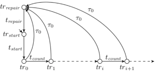
Fig. 4 the (infinite) reachability graph of the SRPN of the figure 3
Definition 9 (Observation graph). Let N = (hP, T, W−, W+i, l, m0) be a labelled marked Petri net. Then the observation graph of
this net is defined by hS, A, m0i where S ⊆ NP, the set of nodes, is
the reachability set of the net, A ⊆ S × Σ × S, the set of edges, and m0 ∈ S, the initial node, is the initial marking of the net. There is an
edge (s, a, s0) ∈ A iff there exists a sequence σ ∈ T∗ such that s−→sσ 0 and l(σ) = a ∈ Σ. Such a sequence is called a witness sequence of the edge.
The proof of the next theorem is based on the reachability graph depicted in figure 4. trstart is the initial extended marking, tri (with
i ∈ N) represents the state of the system where i instructions have been executed and trrepair represents the state where one repairs the
system.
Theorem 1 (Infinite in-degree). Whatever are the labels associ-ated with the SRPN of the figure 3, the graph of the figure 4 cannot be the observation graph of any labelled marked Petri net.
Proof. Assume that there exists a labelled marked Petri net which generates an observation graph isomorphic to the graph of figure 4. Let us denote mi (resp. mrepair) the marking of this net
correspond-ing to the extended markcorrespond-ing tri (resp. trrepair). Since the sequence
m0, m1, . . . includes only distinct markings, we extract from it a
sub-sequence mα(0), mα(1), . . . composed of strictly increasing markings:
∀i < j, ∀p ∈ P, mα(i)(p) ≤ mα(j)(p) ∧ ∃p ∈ P, mα(i)(p) < mα(j)(p). Starting from mα(0), there are at least two witness sequences, one
leading to mrepair (denoted σ) labelled by the cut step τ0 and the
other one leading to mα(0)+1 (denoted σ0). These two sequences are
also enabled from mα(1). Since mα(0) 6= mα(1), σ does not lead to
mrepair and thus necessarily leads to mα(1)+1. Consequently, the
sequence leading from mα(2) to the initial marking m0. As previously
argued, it cannot be σ thus it is σ0. But this sequence leads also from mα(1) to mrepair. Since mα(1) 6= mα(2), there is a contradiction. ut
Stated otherwise, the modelling of crash for a system with an in-finite number of states is impossible with Petri nets. In the restricted case where the system has a finite number of reachable states, it is theoretically possible to model it with a standard Petri net. However, the modelling of a crash requires a number of transitions proportional to the number of reachable states leading to an intricate net. The SRPN design proposed here does not depend on this number and leads to a compact modelling.
2.3 Analysis of SRPNs
Among the numerous approaches to the verification of systems, a typical one consists in first designing a specification model and an implementing one; and then checking whether the two models are bisimilar. Furthermore, as the specification model is often abstract, it can be modelled by a finite automaton. Consequently, this approach raises the problem of bisimulation between a finite automaton and a general transition system.
Whereas checking the bisimulation of two Petri nets is undecid-able [11], checking the bisimulation of a Petri net and a finite au-tomaton becomes decidable [12]. In this subsection, we investigate the generalisation of the latter result to a slightly restricted version of SRPNs.
We will call a restricted sequential recursive Petri net (RSRPN), an SRPN whose sets of final markings are restricted semilinear sets. The expressive power of these RSRPN is still high since the proof that the languages family of the SRPN strictly includes the union of the Petri nets and context-free languages is also valid for RSRPN (see [7]). From a practical point of view, let us notice that the two previous examples of SRPNs are restricted ones and more generally, that modelling termination conditions of subsystems very often yields restricted semilinear sets.
The definitions related to the bisimulation are recalled in the ap-pendix A. Note that restricting the SRPN definition is only required for lemma 2.
Lemma 1. Let (N, tr0) be a marked SRPN, tr be a reachable
ex-tended marking of (N, tr0) and n be a positive integer. Then there
is a reachable extended marking tr0 of (N, tr0) such that (N, tr) ∼n
(N, tr0) and dtr0 ≤ dtr
Proof. If dtr ≤ dtr0 + |Tab| + n, we take tr 0 = tr.
Thus we assume that dtr > dtr0+ |Tab| + n. Consequently, the edges
corresponding to ttr
dtr0, . . . , ttrdtr0+|Tab| have been created by the firing
sequence that leads to tr, say σ. Among them, there are at least two occurrences of the same transition that we will denote t = ttri = ttrj with i < j.
We can express the firing sequence σ like σ = σ0· t · σ1· t · σ2 with the
two occurrences of t corresponding to the production of the labels ttri and ttrj . Now it is straightforward that σ = σ0· t · σ2 is also a firing
sequence leading to an extended marking tr0 with depth strictly less than the one of tr.
As j ≤ dtr0 + |Tab| < dtr − n, the suffixes of length n (counted as
the number of nodes) of the paths corresponding to the extended markings tr and tr0 have identical labels (markings and transitions). Thus due to the semantics of an SRPN, the behaviours of the marked nets (N, tr) and (N, tr0) are identical up to n firings of steps, which implies that (N, tr) ∼n (N, tr0). If the depth of tr0 fulfills dtr0 ≤
dtr0+ |Tab| + n, we are done. Otherwise we iterate this process until
fulfillment. ut
We introduce some notations related to an RSRPN N and to ordinary markings:
• wN is the maximum over the set of valuations of the arcs for input places of transitions, i.e. wN is the least integer such that ∀p ∈ P, ∀t ∈
T, W−(p, t) ≤ wN.
• kN is the maximum over the integers (k, k0, . . .) occurring in the
right sides of the inequalities defining the sets of final markings (see definition 1).
• Let m and m0 be ordinary markings and H be a positive integer. Then m ≈H m0 iff ∀p ∈ P, m(p) = m0(p) ∨ (m(p) ≥ H ∧ m0(p) ≥ H).
The next lemma establishes a sufficient condition for equivalence of two extended markings w.r.t. ∼n. This condition relies on two
observations. First, only the nth last levels of an extended marking determine the firing sequences of length less than or equal to n. Sec-ond, if the marking of a place exceeds some bound depending on n then this place will not disable any firing in such a sequence. More precisely, this lower bound can be set to n · wN + kN + 1.
Lemma 2. Let N be an RSRPN, tr and tr0 be two extended markings of N and n be a positive integer. Let H = n · wN + kN + 1. Assume
that the following assertions are fulfilled: 1. (dtr ≥ n ∧ dtr0 ≥ n) ∨ dtr = dtr0
2. ∀0 < i < min(n, dtr), ttrdtr−i= ttr 0 dtr0−i 3. ∀0 ≤ i < min(n, dtr), mtrdtr−i ≈H mtr 0 dtr0−i Then (N, tr) ∼n(N, tr0).
Proof. Again we notice that the behaviour of an SRPN up to n firings depends only on the suffix of length n of the path corresponding to the extended marking. We prove the lemma by induction on n. The base case n = 0 is trivial. Now assume that n > 0. Let us look at a possible firing in (N, tr). If this firing is an elementary or abstract transition t then t is also enabled in (N, tr0) since, for every p ∈ P , the markings mtrd
tr(p) and m tr0
dtr0(p) are either identical or mtr 0
dtr0(p) ≥ H
does not disable t by definition of H.
Firing t in the two marked nets leads to new extended markings which fulfill the assertion for n − 1. Indeed, the markings where the firing occurs have for a place p either identical markings or a new lower bound (n − 1) · wN+ kN+ 1. The other markings are unchanged
and still satisfy the assertions.
In case where t is an abstract transition, the transition of the new edge is t and the marking of the new node is Ω(t) for both new extended markings.
Let us examine the case of a cut step. We claim that an inequality occurring in the definition of Υ is either satisfied by both mtrdtr and mtrd0
tr0 or not satisfied by both m tr
dtr and m tr0 dtr0.
If this inequality does not involve places with different markings, we are done. Otherwise, let p be such a place i.e. with mtrd
tr(p) 6=
mtrd0
tr0(p) and the corresponding coefficient of the inequality ap 6= 0
(see def. 1). Then these markings are greater than or equal to H and due to the positive coefficients of the inequality, this inequality is not satisfied for both the markings. Hence the evaluation of a boolean combination of inequalities will be identical for the two markings. Thus the cut step is also enabled in (N, tr0). The firing of the cut step leads to two extended markings where the suffixes of length n − 1 still satisfy the assertions (indeed the marking of places in the
new leaf may only be increased). ut
Let H be an integer, an extended marking tr is H-bounded iff ∀p ∈ P, ∀1 ≤ i ≤ dtr, mtri (p) ≤ H. Given tr an H-bounded extended marking, CH(tr) denotes the set of extended markings such that tr0 ∈
CH(tr) iff:
– dtr = dtr0
– ∀1 ≤ i < dtr, ttri = ttr 0 i
ttr0 1 ttr0 2 ttr0 3 ttr0 4 tr0 mtr0 1 mtr0 2 mtr0 3 mtr0 4 mtr0 5 Ω(t) t ∈ Tab ∀i ∈ I, Υi N ? ttr1 tr mtr 1 mtr2 (dtr = 2) (ttr0 1 , 1) (ttr0 2 , 2) (ttr0 3 , 3) (ttr0 4 , 3) tr00 mtr0 1 mtr0 2 + qttr 01 mtr0 3 + qttr 02 mtr0 4 + qttr 03 mtr0 5 + qttr 04 + p3
witness of the generating abstract transition
witness of the current level up to 3 Ω(t) + p2+ qt Ω(t) + p3+ qt Ω(t) + p3+ qt p1 p2 p3 qt (t, 1) (t, 2) (t, 3) ∀i ∈ I, Υ0 i = {m | m|P ∈ Υi∧ m(p1) = 0} N0
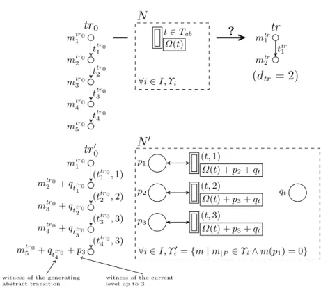
Fig. 5 an illustrative scheme of the construction of lemma 3 (first part)
– ∀1 ≤ i ≤ dtr, mtri ≈H mtr 0 i
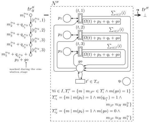
Lemma 3. Let (N, tr0) be a marked SRPN, H be an integer and tr
be a H-bounded extended marking of N . Then one can build a marked SRPN (N00, tr000) such that ⊥ is reachable from (N00, tr000) if and only if there exists an extended marking of CH(tr) reachable from (N, tr0).
Proof. We assume that tr0 6=⊥ since CH(⊥) = {⊥} and, in
conse-quence, we can set (N00, tr000) = (N, tr0).
First, we build an intermediate SRPN (N0, tr00) obtained by a transformation of (N, tr0) (see Figure 5). We add two sets of places
{p1, p2, . . . , pdtr+1} and {qt| t ∈ Tab}. Any abstract transition t
is replaced by dtr + 1 copies (t, 1), (t, 2), . . . , (t, dtr + 1) such that
∀d ≤ dtr + 1, (t, d) has pd as additional input and output place.
These additional arcs are the only ones connected to the new places. Moreover ∀d ≤ dtr, in Ω0((t, d)), pd+1 and qt are marked and in
Ω0((t, dtr+ 1)), pdtr+1 and qt are marked.
tr00 has the same depth as tr0 and ∀d < dtr0, if d ≤ dtr then
ttr 0 0 d = (t tr0 d , d) else t tr00 d = (t tr0
d , dtr+ 1). The markings of nodes of tr 0 0
(ttr0 1 , 1) (ttr0 2 , 2) (ttr0 3 , 3) (ttr0 4 , 3) tr000 mtr0 1 mtr0 2 + qttr 01 mtr0 3 + qttr 02 mtr0 4 + qttr 03 mtr0 5 + qttr 04 + p3+ go
marked during the sim-ulation stage Ω(t) + p2+ qt+ go Ω(t) + p3+ qt+ go Ω(t) + p3+ qt+ go p1 p2 p3 qt go (t, 1) (t, 2) (t, 3) t0∈ Tel P i∈Ihii P i∈Ihii P i∈Ihii N00 ∀i ∈ I, Υ00 i = {m | m|P0 ∈ Υi0∧ m(go) = 1} Υi001 = {m | m(p2) = 1 ∧ m(qttr1) = 1 ∧ m|P ≈H mtr2} Υi002 = {m | m(p2) = 1 ∧ m(go) = 0 ∧ m|P ≈H mtr1} ? ⊥ tr00
Fig. 6 an illustrative scheme of the construction of lemma 3 (second part)
are defined as follows: – ∀1 ≤ d ≤ dtr0, ∀p ∈ P, m tr0 0 d (p) = m tr0 d (p), – ∀t ∈ Tab, m tr00 1 (qt) = 0, – ∀1 < d ≤ dtr0, ∀t ∈ Tab, if t tr0 d−1 = t then m tr0 0 d (qt) = 1 else mtr 0 0 d (qt) = 0, – ∀1 ≤ d ≤ dtr0, ∀1 ≤ d 0 ≤ d tr + 1, if d0 = d = dtr0 ∧ d ≤ dtr then mtr 0 0 d (pd0) = 1 else if d0 = dtr + 1 ∧ d = dtr 0 ∧ d > dtr then mtr 0 0 d (pd0) = 1 else m tr00 d (pd0) = 0.
In the new net, m ∈ Υi0 iff the projection on the original places belong to Υi and p1 is unmarked.
Given a firing sequence of (N, tr0) not leading to ⊥, one can build a
firing sequence of (N0, tr00) by substituting for the firing of an abstract transition t the firing of (t, d) where d = min(d0, dtr+1) and d0denotes
the level where the firing has occurred. Moreover, the intermediate extended markings coincide on places of P and in N0, all places pd
occurring at level k ≤ dtr+ 1, m(pk) = 1 ∧ ∀k0 6= k, m(pk0) = 0 and
in a marking m occurring at level k > dtr+ 1, m(pdtr+1) = 1 ∧ ∀k 0 6=
dtr+ 1, m(pk0) = 0. If this level has been created by the firing of the
abstract transition t then m(qt) = 1 ∧ ∀t0 6= t, m(qt0) = 0. At the root
level, all places qt are unmarked.
Conversely, given a firing sequence of (N0, tr00), one can build a firing sequence of (N, tr0) by substituting for the firing of an abstract
transition (t, d) the firing of t. Moreover the intermediate extended markings coincide on places of P . We also note that no firing sequence of (N0, tr00) leads to ⊥ since at the root level, p1 is marked and every
Υi requires that m(p1) = 0.
Now we make the second transformation leading from (N0, tr00) to the construction of the marked net (N00, tr000) (see Figure 6). We add a new place go. Considering places different from go, tr000 is identical to tr00, ∀1 < d < dtr0, m
tr000
d (go) = 0 and m tr000
dtr0(go) = 1.
Furthermore, ∀t ∈ Tab00, Ω00(t) = Ω0(t)+go. We now partially define the connection between go and the transitions: ∀t ∈ T00, W00−(go, t) = 1 and ∀t ∈ Tel00, W00+(go, t) = 1. The remaining connections will be defined within the presentation of the new set of indices.
This set is I00 = I ∪ {i1, i2}. ∀i ∈ I, m ∈ Υi00 iff m(go) = 1 and
the projection on the other places belongs to Υi0. And ∀i ∈ I, ∀t ∈ Tab0 , W00+(go, t, i) = 1. Υi00
1 is the set of markings m 0 s.t.:
– m0(pdtr) = 1,
– dtr > 1 ⇒ m0(qttr
dtr−1) = 1,
– mtrdtr ≈H m0|P.
Thus this cut step is only enabled at the level dtr. Υi002 is the set of
markings m0 s.t. ∃1 ≤ d < dtr : – m0(pd) = 1, – d > 1 ⇒ m0(qttr d−1) = 1, – mtrd ≈H m0|P, – m0(go) = 0.
Thus this cut step is only enabled at the levels 1 ≤ d < dtr.
These two cut steps do not produce any token: ∀p ∈ P00, t ∈ Tab00, i ∈ {i1, i2}, W00+(p, t, i) = 0.
Let σ be a firing sequence of (N00, tr000) which does not include τi1 and τi2 steps. This sequence corresponds to a firing sequence of
the original net with the following additional informations: in every visited extended marking, the marking of places pdwitnesses the level
qt indicates which abstract transition has created the level and the
place go is marked only at the higher level. Similarly, a firing sequence of the original net (which does not lead to ⊥) can be simulated in (N00, tr000) with the same additional informations.
Since a τi2 step requires the place go to be unmarked it can only
be fired if at level dtr there has been a τi1 step.
Thus the behaviour of this net is the following one: it simulates the original net until it reaches an extended marking tr00 corresponding to an extended marking tr0 of the original net with dtr0 = dtr such
that at this level , tr0 fulfills the condition of CH(tr) related to level
dtr, i.e. ttrdtr−1 = ttr 0 dtr−1 and m tr dtr ≈H m tr0 dtr which is equivalent to mtrd00 tr ∈ Υ 00 i1.
Then it performs a cut step τi1. The simulation is now stopped
(the place go is unmarked) and the execution can only produce τi2
steps until ⊥ is reached iff at every level k decreasing from dtr− 1 to
1 all the intermediate markings and abstract transitions firings of tr0 fulfill the conditions of CH(tr) related to k, i.e. ttrk−1 = ttr
0
k−1 (when
k > 1) and mtrk ≈H mtrk0.
When the net stops the simulation, the current extended marking may not correspond to an extended marking of CH(tr). In this case,
the net will reach a deadlock different from ⊥ since one of the τi2
step will not be enabled.
Thus ⊥ is reachable in (N00, tr000) iff an extended marking of CH(tr)
is reachable from (N, tr0). ut
In order to state the main result of this section, we introduce tran-sition labels defined by a label mapping l. l(t), the label of trantran-sition t, is either a letter of a finite alphabet or the empty word. Cut steps are similarly labelled by l. We note tr0−→l(t)Ntr1 whenever tr0−→t Ntr1.
Theorem 2 (Bisimulation of an RSRPN). The problem of bisim-ulation between a labelled marked RSRPN (N, l, tr0) where no
transi-tion or cut step is labelled by the empty word and a finite transitransi-tion system (LT S, s0) is decidable.
Proof. Let n be the number of states of LT S. Due to lemma 6 of the appendix A, it suffices to check whether (N, l, tr0) ∼n(LT S, s0) and
whether there exists an extended marking tr1 reachable from tr0 s.t.
tr1 ∈ IncLT Sn .
In order to check (N, l, tr0) ∼n(LT S, s0), we verify that:
1. for every step tr0−→a Ntr1, there exists s1 s.t. s0−→a LT Ss1 and
2. for every s1 s.t. s0−→a LT Ss1, there exists a step tr0−→a Ntr1 s.t.
(N, l, tr1) ∼n−1(LT S, s1).
These conditions straightforwardly lead to a recursive procedure where the number of nested calls is bounded by n.
Due to lemma 1, in order to check whether there exists tr1 reachable
from tr0 s.t. tr1 ∈ IncLT Sn we can restrict the search to extended
markings whose depth is bounded by dtr0 + |Tab| + n.
Due to lemma 2, each such extended marking tr1 belongs to some
CH(tr) with H = n · wN + kN + 1 and tr being H-bounded, whose
depth is bounded by dtr0 + |Tab| + n and such that (N, l, tr) ∼n
(N, l, tr1). More precisely, dtr = dtr1, ∀1 ≤ d < dtr, t tr d = t tr1 d and ∀1 ≤ d ≤ dtr, ∀p ∈ P, mtrd1(p) ≤ H ⇒ mtrd(p) = m tr1 d (p) and m tr1 d (p) > H ⇒ mtrd(p) = H.
Let us call T R the set of H-bounded extended markings whose depth is bounded by dtr0 + |Tab| + n. This set is finite. For each
tr ∈ T R, we check whether an extended marking of CH(tr) is
reach-able in (N, tr0) using the procedure described in lemma 3: we
re-duce it to a reachability problem for (N00, tr000) (decidable by theo-rem 3 to be shown in section 3.4 for general recursive Petri nets). If some tr0 ∈ CH(tr) is reachable then using the procedure described
in the beginning of the proof, we check for every state s ∈ LT S whether (N, l, tr) ∼n(LT S, s). If no s is found for some tr ∈ T R then
(N, l, tr) ∈ IncLT Sn and since (N, l, tr0) ∼n(N, l, tr) then (N, l, tr0) ∈
IncLT S
n . So the second condition of lemma 6 is not fulfilled when
some tr0 ∈ CH(tr) is reachable from tr0. The algorithm 1 describes
the procedure associated with this proof. ut Observation. In order to abstract the call mechanism, it would be in-teresting to hide abstract transitions and cut steps by labelling them with the empty word. Unfortunately, the problem of the bisimulation between a Petri net with some empty labels and a LTS is already undecidable [12]. A partial solution would be to label such items by specific labels (e.g. “call” and “return”).
3 Recursive Petri Nets
Discussion. Let us emphasize the applicability and limits of SRPNs. They are appropriate when dealing with real-time systems composed by several static tasks ranked by execution level or with collaborative applications where the interactions are based on synchronous remote procedure calls. However, as soon as the tasks can be dynamically
Algorithm 1: CheckBisimulation
input : a marked RSRPN (N, tr0) and a finite LTS (LT S, s0)
output: a boolean indicating if (N, tr0) ∼ (LT S, s0)
CheckBisimulation() begin
//n is the number of states of LT S
return CheckCond1(tr0, s0, n) and CheckCond2();
end
CheckCond1(tr, s, l) begin if l == 0 then return true; foreach tr−→a Ntr1do
if not (∃s1 s.t. s−→a LT Ss1 and CheckCond1(tr1, s1, l − 1)) then
return false; end
end
foreach s−→a LT Ss1 do
if not (∃tr1 s.t. tr−→a Ntr1 and CheckCond1(tr1, s1, l − 1)) then
return false; end end return true; end CheckCond2() begin
foreach H-bounded tr0 whose depth is bounded by dtr+ |Tab| + n do
//using lemma 3
//and the reachability procedure for RPNs if CheckReach(tr0, CH(tr0)) then
found = false;
foreach state s0 of LT S do
found = found or CheckCond1 (tr0, s0, n); end
if not found then return false; end
end
return true; end
created or the calls are asynchronous, the SRPN model is not enough powerful. This motivates the introduction of recursive Petri nets.
3.1 Definitions
SRPNs enlarge Petri nets by introducing a “function call” like mech-anism. However, concurrency (the main feature of Petri nets) is con-fined inside the single active node. In Recursive Petri Nets (RPNs), all the nodes are active and therefore concurrency also occurs between
node activities. Thus, in an RPN there is a tree of threads (denoting the fatherhood relation) where all the threads play their own token game. A step of an RPN is thus a step of one of its threads. This has an immediate consequence on the cut steps: when a thread performs a cut step the subtree whose root it is pruned.
Furthermore, RPNs include additional mechanisms which enable the modeler to express various kinds of control between threads.
– Place capacities: Each place has a specific bound on the number of tokens it can contain. This bound may be infinite meaning that there is no constraint on the place. The set of places with a finite bound is denoted Q.
– Test arcs: A new kind of arcs, called test arcs, checks for the exact number of tokens in a place. This place must belong to Q (see the end of this section for a discussion about test arcs). – Variable starting markings: The starting marking of an
ab-stract transition may depend on the current ordinary marking of the thread which fires it. More precisely, this dependence is re-stricted to the submarking of places in Q.
– Thread interrupts: The behaviour of an elementary transition is now twofold and depends on a partial function which associates with it, a set of abstract interrupted transitions and the indexes of the termination. Thus on the one hand, an elementary transition consumes and produces the tokens specified by the backward and forward matrices as an elementary transition of an SRPN. On the other hand, it deletes some subtrees according to the partial function.
The next definitions formalise the syntax and the semantics of RPNs.
Definition 10 (Recursive Petri nets). A recursive Petri net is defined by a tuple N = hP, B, T, I, W−, W∗, W+, Ω, Υ, Ki where
– P is a finite set of places,
– B is the bounding function from P to N ∪ {∞} inducing the fol-lowing notations:
– Q = {p ∈ P | B(p) 6= ∞} the subset of bounded places, – B[Q] = {m ∈ NQ| ∀q ∈ Q, m(q) ≤ B(q)},
– B[P ] = {m ∈ NP | ∀p ∈ P, m(p) ≤ B(p)},
– T is a finite set of transitions such that P ∩ T = ∅,
– a transition of T can be either elementary or abstract. The sets of elementary and abstract transitions are respectively denoted by Tel and Tab,
– I is a finite set of indexes,
– W− is the pre function from P × T to N,
– W∗ is the test partial function from Q × T to N,
– W+ is the post function from P × [Tel∪ (Tab× I)] to N,
– Ω is the starting marking function from Tab× B[Q] to B[P ],
– Υ is a family indexed by I of effective representations of semilinear sets of final markings,
– K is a partial function from Tel× Tab to I such that ∀t ∈ Tab,
(∃t0 ∈ Tel, K(t0, t) is defined ⇒
∀p ∈ Q, W−(p, t) = 0, ∀i ∈ I, W+(p, t, i) = 0).1
Notations and terminology:
– Let t be an abstract transition, K(t) denotes the set of elementary transitions which interrupt t (i.e. K(t) = {t0| K(t0, t) is defined}). Remark that the index relative to an interrupt is deterministically selected contrary to the index of the cut steps.
– Let t be an elementary transition, K(t) denotes the set of abstract transitions which are interrupted by t
(i.e. K(t) = {t0| K(t, t0) is defined}). – We denote by Q the set P \ Q.
– We will often focus on the subnet generated by Q. Thus we in-troduce a useful abbreviation. Let t be a transition and m a sub-marking on Q then m is compatible with t iff ∀q ∈ Q, (W∗(q, t) is undefined or m(q) = W∗(q, t)) and m(q) ≥ W−(q, t).
Definition 11 (Extended marking). An extended marking tr of a recursive net N = hP, B, T, I, W−, W∗, W+, Ω, Υ, Ki is a labelled rooted tree directed from the root to the leaves tr = hV, M, E, Ai where – V is the (possibly empty) finite set of nodes. When it is non empty
v0 ∈ V denotes the root of the tree,
– M is a mapping from V to NP associating an ordinary marking with any node and such that ∀v ∈ V, ∀p ∈ P, M (v)(p) ≤ B(p), – E ⊆ V × V is the set of edges,
– A is a mapping from E to Tab associating an abstract transition
with any edge.
A marked recursive Petri net (N, tr0) is a recursive Petri net N
together with an initial extended marking tr0. 1
The requirement that an interruptible abstract transition does not modify the marking of places of Q will be used for the proof of the decidability of the reachability problem (see the first part of the proof of the lemma 5).
When we deal with different extended markings, we will denote the items of an extended marking tr as a function (e.g. V (tr)) and more particulary, when tr is non empty, we denote by v0(tr) the root node.
For any node v ∈ V , we denote by Succ(v) the set of its direct and indirect successors including v (∀v ∈ V, Succ(v) = {v0 ∈ V | (v, v0) ∈
E∗} where E∗ stands for the reflexive and transitive closure of E). Moreover, when v is not the root of the tree, we denote by pred (v) its (unique) predecessor. The empty tree is denoted by ⊥. Any ordinary marking m can be seen as an extended marking, denoted by dme, consisting of a single node.
An elementary step of an RPN may be either a firing of a transition or a cut step (denoted by τi with i ∈ I).
Definition 12. The firing of an elementary transition t from a node v of an extended marking tr = hV, M, E, Ai leads to the extended marking tr0= hV0, M0, E0, A0i (denoted by tr−→trt,v 0) if and only if: Let E00= {(v, v0) ∈ E|A((v, v0)) ∈ K(t)} and V00 = {v0 ∈ V |(v, v0) ∈ E00},
– ∀p ∈ P, M (v)(p) ≥ W−(p, t),
– ∀q ∈ Q s.t. W∗(q, t) is defined, M (v)(q) = W∗(q, t), – V0= V \ (∪v0∈V00Succ(v0)), E0 = E ∩ (V0× V0),
– ∀e ∈ E0, A0(e) = A(e), ∀v0 ∈ V0\ {v}, M0(v0) = M (v0),
– ∀p ∈ P, M0(v)(p) = M (v)(p) − W−(p, t) + W+(p, t) +
Σe∈E00W+(p, A(e), K(t, A(e))).
Definition 13. The firing of an abstract transition t from a node v of an extended marking tr = hV, M, E, Ai leads to the extended mark-ing tr0 = hV0, M0, E0, A0i (denoted by tr−→trt,v 0) if and only if:
Let v0 be a fresh identifier, – ∀p ∈ P, M (v)(p) ≥ W−(p, t),
– ∀q ∈ Q s.t. W∗(q, t) is defined, M (v)(q) = W∗(q, t), – V0= V ∪ {v0} , E0 = E ∪ {(v, v0)},
– ∀e ∈ E, A0(e) = A(e), A0((v, v0)) = t, – ∀v00∈ V \ {v}, M0(v00) = M (v00),
– ∀p ∈ P, M0(v)(p) = M (v)(p) − W−(p, t), – M0(v0) = Ω(t, M (v)|Q).
Definition 14. The firing of a cut step τi from a node v of an
ex-tended marking tr = hV, M, E, Ai leads to the exex-tended marking tr0= hV0, M0, E0, A0i (denoted by trτi,v
M (v) ∈ Υi and if v is the root of the tree then tr0=⊥, otherwise:
– V0= V \ Succ(v), E0= E ∩ (V0× V0), ∀e ∈ E0, A0(e) = A(e), – ∀v0 ∈ V0\ {pred (v)}, M0(v0) = M (v0),
– ∀p ∈ P, M0(pred (v))(p) = M (pred (v))(p)+W+(p, A(pred (v), v), i). Let tr−→trs,v 0 be a firing, then s is said to be an enabled step in v, denoted by tr−→. Other notations about firing sequences and reach-s,v ability in SRPNs are carried over RPNs.
Remarks:
– i ∈ I represents a possible effect (see the domain of function W+) consecutive to a subtree pruning. There are two ways to prune a subtree: by a cut step when the ordinary marking of the subtree root belongs to Υi or by the firing of an elementary transition t
which interrupts t0, the transition labelling the edge to the subtree (i.e. K(t, t0) = i). When Υi is the empty set this means that the
index i can only be the effect of an interrupt.
– The bounding constraint on places of Q is implicitly taken into ac-count by requiring that tr0 introduced in definitions 12, 13 and 14 is an extended marking (see the second item of definition 11). – Since in the previous definitions, an elementary step requires the
tree is not empty, the extended marking ⊥ is dead.
– Inhibitor arcs connected to bounded places could be easily simu-lated by test arcs. Due to the boundedness requirement, this does not lead to undecidability for the reachability problem.
We now justify the introduction of test arcs in the model. In or-dinary Petri nets, a test arc on a bounded place can be simulated by the introduction of a complementary place which records the differ-ence between the bound and the current marking such that an input arc from the original place generates an output arc to this place and vice versa. Then, a test arc is transformed in two loops around the two places, respectively labelled by the tested value and its difference with the bound.
Such a construction is no more valid when the test arc is connected to an abstract transition since then the consuming and producing of tokens are performed in two distinct steps. Indeed, the effect of W+ is delayed until a cut step occurs in the new thread or an elementary transition is fired which interrupts the thread subtree initiated by the abstract transition.
Furthermore, note that according to semantics ∀p ∈ P, ∀t ∈ T when defined W∗(p, t) ≥ W−(p, t) since otherwise the transition t will never be enabled.
Although the semantics of SRPN and RPN are different, any marked SRPN (N, tr0) can be simulated by a marked RPN (N0, tr00)
in such a way that the standard equivalent relations are fulfilled by the two nets (bisimulation, language equivalence, reachability graph isomorphism, etc). The construction is straightforward, so we infor-mally describe it. First N0 is a copy of N . Then a control place is added to N0 and is both an input and a output place of every transi-tion. The starting marking of any abstract transition is equal to the original one plus a token in this control place. Similarly, tr00 is a copy of tr0 with the control place marked only in the active node.
3.2 An illustrative example
The net of figure 7 illustrates the characteristic features of RPNs. The items which are absent in SRPNs are represented graphically as follow:
– a place of Q by a double border circle whose bound is indicated in brackets after its name and
– a test arc between a place p and a transition t by a simple line. This line is labelled with W∗(p, t) when W∗(p, t) 6= 1.
The name of an elementary transition t is followed by the set {t0hii | K(t, t0) = i} when this set is non empty. The starting marking of an abstract transition is defined by a mapping from a finite domain to the set of ordinary markings. So the modeler could define it by an enumeration. However for our examples, we adopt a more concise way to specify it. Given an abstract transition t, its starting marking mapping is indicated in a frame with the following syntax: Σp∈P[Ωp,t]·
p where Ωp,t is an arithmetical expression involving the variables
{q | q ∈ Q}. Given a current submarking m on Q and a place p the value of Ω(t, m)(p) is obtained by evaluating the expression where any variable q is replaced by m(q). Here again, when Ωp,tis null the term
[Ωp,t]·p is omitted and is abbreviated to p when Ωp,t= 1. For instance,
[prec− 1] · prec+ pint means that the starting marking m of a node
created by firing tf ork will be defined by ∀p ∈ P \ {pint, prec}, m(p) =
0, m(pint) = 1 and m(prec) = v − 1 where v is the number of tokens
in place prec in the marking of the node where the firing occurs.
The net in figure 7 shows the modelling of similar transactions performed by a remote server. A transaction is started by the fir-ing of the transition tstart. The status of the server is described by
the places On and Off . Thus, the firing of tstart is controlled by a
[2] · prec+ pinit {tstarth1i} On(1) Off treset tset pstart tstart poutput toutput h0i h1i
[prec− 1] · prec+ pinit
prec(2) pinit tfork tlocal pend h0i Υ0= {m | m(pend) > 0} Υ1= ∅
Fig. 7 a simple recursive Petri net
(represented by the index h0i) or abort when the server is reset (rep-resented by the index h1i). Since there are two ways to terminate a transaction, I includes two items (I = {0, 1}). In the first case, the termination of a transaction is indicated by a token in pend (see Υ0).
Then the cut step puts a token in the place poutput which controls
the transition toutput modelling the transmission of the result. In the
second case, the abortion is modelled by the transition treset which
interrupts tstart with the index h1i. This firing produces a token in
place pstart meaning that the transaction does not provide a result.
Υ1 is empty since the abortion is never triggered by the execution of
the transaction but only when the server is reset. If the modelling of faults would be required, it could be introduced by additional places and modifying Υ1.
When started, a transaction may proceed locally by firing tlocal
or starts a new process by firing tfork. The place prec controls the
maximal number of nested forks. The starting marking of tstart
ex-presses that there will be at most two forks per transaction. Note that a thread initiated by the transition tfork has an initial marking
with one token less in the place prec than its initiator. The abortion
process realised by the transition treset applies on the whole
transac-tions i.e. in the root of the reached extended markings. It is easy to see that in another node the transition treset is never enabled.
Notice that the bounded places are On and prec. Thus, this net
fulfills the conditions of def. 10: the single test arc is connected to On and starting marking of tfork depends exclusively on prec.
2 · pstart+ On tstart pstart+ On 2 · prec+ pinit tstart tstart tstart On 2 · prec+ pinit 2 · prec+ pinit tstart tstart tstart On 2 · prec+ pinit 2 · prec+ pend tlocal tstart tstart tfork On prec 2 · prec+ pend prec+ pinit tfork tstart tfork poutput+ On prec prec+ pinit τ0
pstart+ poutput+ Off
treset
2 · pstart+ Off
toutput
Fig. 8 a firing sequence
The initial state of the net is a tree reduced to a single node with two tokens in pstart corresponding to two transactions to begin and
one token in On indicating that the server is operational. A firing sequence of this marked RPN is presented in the figure 8. The arcs of the trees composing the visited extended markings are labelled by the abstract transition tstart for the outgoing arcs from the root and
by tf ork for the other ones. The black node of an extended marking
denotes the thread initiator of the current step. Let us notice that each firing of an abstract transition leads to the creation of a new node in the tree whereas the firing of the cut step prunes the subtree of the root represented in the figure as its right branch. Moreover the firing of the elementary transition treset prunes its remaining subtree
by the interrupt mechanism.
3.3 Expressivity of RPNs
Modelling of asynchronous remote procedure calls: The procedure we model has a non negative integer as input and returns whether this parameter is odd or even. During the computation the caller is not suspended and for instance may modify the variable which has been transmitted (by value) to the procedure.
The caller consists in two processes: the first one, modelled by the subnet on the left part of the figure 9, iteratively calls the procedure whereas the second one, modelled by the subnet on the central part,
[x] · p + zero idle t A B x(3) p zero one h0i h1i Υ0= {m | m(p) = 0 ∧ m(zero) = 1} Υ1= {m | m(p) = 0 ∧ m(one) = 1}
Fig. 9 an asynchronous remote procedure call example
idle t0 t1 t2 t3 A B x 0 1 2 3
Fig. 10 a Petri net modelling of the parity test
increments or decrements the value of variable x in the interval [0, 3]. The current value of the variable x is denoted by the marking of the eponymous place. The procedure call is represented by the firing of the abstract transition t. Its starting marking “copies” the value of x in place p. The result returned by the procedure is specified by the index of the reached final marking set labelling the output arcs of t: the post condition of t produces a token either in the place A or in B with respect to the final marking reached by the thread initiated by t.
The procedure is modelled by the subnet on the right part of fig-ure 9. This subnet determines whether the starting marking of the place p is even (by reaching a marking of Υ0) or not (by reaching a
marking of Υ1). Notice that the process which updates x is not
sus-pended during the call and then the marking of x can evolve between the firing of t and the firing of the corresponding cut step.
pgo {tstarth1i} pinit(1) tstart pnormal pemergency temergency pgo pend h0i h1i Υ0= {m | m(pend) = 1} Υ1= ∅
Fig. 11 an emergency reaction
The modelling of this pattern by a Petri net raises the problem consisting in assigning the marking of a place to the marking of an-other place (representing the transmission of a parameter). To the best of our knowledge, even when places are bounded, there is no structural solution, i.e. the nets modelling such a pattern depend on the bounds of the places.
The figure 10 presents one possible modelling of the asynchronous remote procedure call by a Petri net. Since the place x is bounded, we have used the test arcs in order to obtain a concise model. With the help of a complementary place, each test arc connected to some ti could be replaced by two loops connecting, on the one hand, tiand
x and, on the other hand, ti and the complementary place of x.
Our solution uses B(x) + 1 transitions (one per possible marking of x) to return the result of the procedure. It is an open question even in this particular case whether a Petri net may be designed independently of the bound of x (here 3).
Modelling of emergency situations: The activity scheduling of an em-bedded critical system depends on the behaviour of the environment. When an emergency situation is encountered, non critical activities are aborted in order to react to this situation. Let us describe how to model such a system with RPNs.
The net of figure 11 represents a system which can initiate any number of tasks by firing tstart. Each task is abstracted by the trivial
subnet at the right of the figure. At any time, transition temergency is
enabled in the root of the extended marking and its firing interrupts all the subtrees initiated at this level. The tasks may also achieve their execution. The two kinds of termination are distinguished by the corresponding indexes of the RPN similarly to the net of figure 7. Assume a current extended marking with n executions of tasks, i.e. a