1
Bayesian Modelling and Inference on
Mixtures of Distributions
Jean-Michel Marin, Kerrie Mengersen and Christian
P. Robert
1‘But, as you have already pointed out, we do not need any more disjointed clues,’ said Bartholomew. ‘That has been our problem all along: we have a mass of small facts and small scraps of information, but we are unable to make any sense out of them. The last thing we need is more.’
Susanna Gregory, A Summer of Discontent
1.1 Introduction
Today’s data analysts and modellers are in the luxurious position of being able to more closely describe, estimate, predict and infer about complex systems of interest, thanks to ever more powerful computational methods but also wider ranges of modelling distributions. Mixture models constitute a fascinating illustration of these aspects: while within a parametric family, they offer malleable approximations in non-parametric settings; although based on standard distributions, they pose highly complex computational challenges; and they are both easy to constrain to meet identifiability re-quirements and fall within the class of ill-posed problems. They also provide an endless benchmark for assessing new techniques, from the EM algo-rithm to reversible jump methodology. In particular, they exemplify the
1Jean-Michel Marin is lecturer in Universit´e Paris Dauphine, Kerrie Mengersen
is professor in the University of Newcastle, and Christian P. Robert is professor in Universit´e Paris Dauphine and head of the Statistics Laboratory of CREST. K. Mengersen acknowledges support from an Australian Research Council Dis-covery Project. Part of this chapter was written while C. Robert was visiting the Australian Mathematical Science Institute, Melbourne, for the Australian Re-search Council Center of Excellence for Mathematics and Statistics of Complex Systems workshop on Monte Carlo, whose support he most gratefully acknowl-edges.
formidable opportunity provided by new computational technologies like Markov chain Monte Carlo (MCMC) algorithms. It is no coincidence that the Gibbs sampling algorithm for the estimation of mixtures was proposed
before (Tanner and Wong 1987) and immediately after (Diebolt and Robert
1990c) the seminal paper of Gelfand and Smith (1990): before MCMC was popularised, there simply was no satisfactory approach to the computation of Bayes estimators for mixtures of distributions, even though older impor-tance sampling algorithms were later discovered to apply to the simulation of posterior distributions of mixture parameters (Casella et al. 2002).
Mixture distributions comprise a finite or infinite number of components, possibly of different distributional types, that can describe different features of data. They thus facilitate much more careful description of complex sys-tems, as evidenced by the enthusiasm with which they have been adopted in such diverse areas as astronomy, ecology, bioinformatics, computer science, ecology, economics, engineering, robotics and biostatistics. For instance, in genetics, location of quantitative traits on a chromosome and interpreta-tion of microarrays both relate to mixtures, while, in computer science, spam filters and web context analysis (Jordan 2004) start from a mixture assumption to distinguish spams from regular emails and group pages by topic, respectively.
Bayesian approaches to mixture modelling have attracted great interest among researchers and practitioners alike. The Bayesian paradigm (Berger 1985, Besag et al. 1995, Robert 2001, see, e.g.,) allows for probability state-ments to be made directly about the unknown parameters, prior or expert opinion to be included in the analysis, and hierarchical descriptions of both local-scale and global features of the model. This framework also allows the complicated structure of a mixture model to be decomposed into a set of simpler structures through the use of hidden or latent variables. When the number of components is unknown, it can well be argued that the Bayesian paradigm is the only sensible approach to its estimation (Richardson and Green 1997).
This chapter aims to introduce the reader to the construction, prior mod-elling, estimation and evaluation of mixture distributions in a Bayesian paradigm. We will show that mixture distributions provide a flexible, para-metric framework for statistical modelling and analysis. Focus is on meth-ods rather than advanced examples, in the hope that an understanding of the practical aspects of such modelling can be carried into many disci-plines. It also stresses implementation via specific MCMC algorithms that can be easily reproduced by the reader. In Section 1.2, we detail some ba-sic properties of mixtures, along with two different motivations. Section 1.3 points out the fundamental difficulty in doing inference with such objects, along with a discussion about prior modelling, which is more restrictive than usual, and the constructions of estimators, which also is more in-volved than the standard posterior mean solution. Section 1.4 describes the completion and non-completion MCMC algorithms that can be used
for the approximation to the posterior distribution on mixture parameters, followed by an extension of this analysis in Section 1.5 to the case in which the number of components is unknown and may be estimated by Green’s (1995) reversible jump algorithm and Stephens’ 2000 birth-and-death pro-cedure. Section 1.6 gives some pointers to related models and problems like mixtures of regressions (or conditional mixtures) and hidden Markov models (or dependent mixtures), as well as Dirichlet priors.
1.2 The finite mixture framework
1.2.1 Definition
The description of a mixture of distributions is straightforward: any convex combination (1.1) k X i=1 pifi(x) , k X i=1 pi = 1 k > 1 ,
of other distributions fi is a mixture. While continuous mixtures
g(x) =
Z
Θ
f (x|θ)h(θ)dθ
are also considered in the literature, we will not treat them here. In most cases, the fi’s are from a parametric family, with unknown parameter θi, leading to the parametric mixture model
(1.2)
k X i=1
pif (x|θi) .
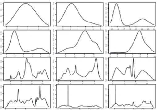
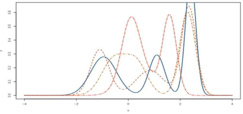
In the particular case in which the f (x|θ)’s are all normal distributions, with θ representing the unknown mean and variance, the range of shapes and features of the mixture (1.2) can widely vary, as shown2 by Figure 1.
Since we will motivate mixtures as approximations to unknown distribu-tions (Section 1.2.3), note at this stage that the tail behaviour of a mixture is always described by one or two of its components and that it therefore reflects the choice of the parametric family f (·|θ). Note also that the repre-sentation of mixtures as convex combinations of distributions implies that
2To draw this set of densities, we generated the weights from a Dirichlet
D(1, . . . , 1) distribution, the means from a uniform U [0, 5 log(k)] distribution, and the variances from a Beta Be(1/(0.5 + 0.1 log(k)), 1), which means in partic-ular that the variances are all less than 1. The resulting shapes reflect this choice, as the reader can easily check by running her or his own simulation experiment.
−1 0 1 2 3 0.1 0.2 0.3 0.4 0 1 2 3 4 5 0.0 0.1 0.2 0.3 0.4 0.51.0 1.5 2.0 2.5 3.03.5 4.0 0.0 0.2 0.4 0.6 0.8 1.0 0 2 4 6 8 10 0.00 0.10 0.20 0.30 0 2 4 6 0.00 0.05 0.10 0.15 0.20 0.25 −2 0 2 4 6 8 10 0.00 0.10 0.20 0.30 0 5 10 15 0.00 0.05 0.10 0.15 0 5 10 15 0.00 0.05 0.10 0.15 0 5 10 15 0.00 0.05 0.10 0.15 0.00 0.05 0.10 0.15 0.0 0.2 0.4 0.6 0.8 1.0 0.0 0.1 0.2 0.3
FIGURE 1. Some normal mixture densities for K = 2 (first row), K = 5 (second
row), K = 25 (third row) and K = 50 (last row).
the moments of (1.1) are convex combinations of the moments of the fj’s: E[Xm] =
k X i=1
piEfi[Xm] .
This fact was exploited as early as 1894 by Karl Pearson to derive a moment estimator of the parameters of a normal mixture with two components, (1.3) p ϕ (x; µ1, σ1) + (1 − p) ϕ (x; µ2, σ2) .
where ϕ(·; µ, σ) denotes the density of the N (µ, σ2) distribution.
Unfortunately, the representation of the mixture model given by (1.2) is detrimental to the derivation of the maximum likelihood estimator (when it exists) and of Bayes estimators. To see this, consider the case of n iid observations x = (x1, . . . , xn) from this model. Defining p = (p1. . . , pk)
and theta = (θ1, . . . , θk), we see that even though conjugate priors may be used for each component parameter (pi, θi), the explicit representation of the corresponding posterior expectation involves the expansion of the likelihood (1.4) L(θ, p|x) = n Y i=1 k X j=1 pjf (xi|θj)
into kn terms, which is computationally too expensive to be used for more than a few observations (see Diebolt and Robert 1990a,b, and Section 1.3.1). Unsurprisingly, one of the first occurrences of the Expectation-Maximization (EM) algorithm of Dempster et al. (1977) addresses the problem of solving the likelihood equations for mixtures of distributions, as detailed in Section 1.3.2. Other approaches to overcoming this compu-tational hurdle are described in the following sections.
1.2.2 Missing data approach
There are several motivations for considering mixtures of distributions as a useful extension to “standard” distributions. The most natural approach is to envisage a dataset as constituted of several strata or subpopulations. One of the early occurrences of mixture modeling can be found in Bertillon (1887) where the bimodal structure on the height of (military) conscripts in central France can be explained by the mixing of two populations of young men, one from the plains and one from the mountains (or hills). The mixture structure appears because the origin of each observation, that is, the allocation to a specific subpopulation or stratum, is lost. Each of the
xi’s is thus a priori distributed from either of the fj’s with probability pj. Depending on the setting, the inferential goal may be either to reconstitute the groups, usually called clustering, to provide estimators for the param-eters of the different groups or even to estimate the number of groups.
While, as seen below, this is not always the reason for modelling by mix-tures, the missing structure inherent to this distribution can be exploited as a technical device to facilitate estimation. By a demarginalization ar-gument, it is always possible to associate to a random variable X from a mixture of k distributions (1.2) another random variable Zi such that (1.5) Xi|Zi= z ∼ f (x|θz), Zi ∼ Mk(1; p1, ..., pk) ,
where Mk(1; p1, ..., pk) denotes the multinomial distribution with k modal-ities and a single observation. This auxiliary variable identifies to which component the observation xi belongs. Depending on the focus of infer-ence, the Zi’s will or will not be part of the quantities to be estimated.3
1.2.3 Nonparametric approach
A different approach to the interpretation and estimation mixtures is semi-parametric. Noticing that very few phenomena obey the most standard dis-tributions, it is a trade-off between fair representation of the phenomenon and efficient estimation of the underlying distribution to choose the rep-resentation (1.2) for an unknown distribution. If k is large enough, there is support for the argument that (1.2) provides a good approximation to most distributions. Hence a mixture distribution can be approached as a type of basis approximation of unknown distributions, in a spirit similar to wavelets and such, but with a more intuitive flavour. This argument will be pursued in Section 1.3.5 with the construction of a new parameterisation
3 It is always awkward to talk of the Z
i’s as parameters because, on the one
hand, they may be purely artificial, and thus not pertain to the distribution of the observables, and, on the other hand, the fact that they increase in dimension at the same speed as the observables creates a difficulty in terms of asymptotic validation of inferential procedures (Diaconis and Freedman 1986). We thus prefer to call them auxiliary variables as in other simulation setups.
of the normal mixture model through its representation as a sequence of perturbations of the original normal model.
Note first that the most standard non-parametric density estimator, namely the Nadaraya–Watson kernel (Hastie et al. 2001) estimator, is based on a (usually Gaussian) mixture representation of the density,
ˆ kn(x|x) = 1 nhn n X i=1 ϕ (x; xi, hn) ,
where x = (x1, . . . , xn) is the sample of iid observations. Under weak
con-ditions on the so-called bandwidth hn, ˆkn(x) does converge (in L2norm and
pointwise) to the true density f (x) (Silverman 1986).4
The most common approach in Bayesian non-parametric Statistics is to use the so-called Dirichlet process distribution, D(F0, α), where F0 is
a cdf and α is a precision parameter (Ferguson 1974). This prior distri-bution enjoys the coherency property that, if F ∼ D(F0, α), the vector
(F (A1), . . . , F (Ap)) is distributed as a Dirichlet variable in the usual sense
Dp(αF0(A1), . . . , αF0(Ap))
for every partition (A1, . . . , Ap). But, more importantly, it leads to a
mix-ture representation of the posterior distribution on the unknown distribu-tion: if x1, . . . , xn are distributed from F and F ∼ D(F0, α), the marginal
conditional cdf of x1 given (x2, . . . , xn) is µ α α + n − 1 ¶ F0(x1) + µ 1 α + n − 1 ¶Xn i=2 Ixi≤x1.
Another approach is to be found in the Bayesian nonparametric pa-pers of Verdinelli and Wasserman (1998), Barron et al. (1999) and Petrone and Wasserman (2002), under the name of Bernstein polynomials, where bounded continuous densities with supports on [0, 1] are approximated by (infinite) Beta mixtures
X
(αk,βk)∈N2+
pkBe(αk, βk) ,
with integer parameters (in the sense that the posterior and the predictive distributions are consistent under mild conditions). More specifically, the prior distribution on the distribution is that it is a Beta mixture
k X j=1
ωkjBe(j, k + 1 − j)
4A remark peripheral to this chapter but related to footnote 3 is that the
with probability pk = P(K = k) (k = 1, . . .) and ωkj = F (j/k) − F (j − 1/k) for a certain cdf F . Given a sample x = (x1, . . . , xn), the associated
predictive is then ˆ fn(x|x) = ∞ X k=1 Eπ[ωkj|x] Be(j, k + 1 − j) P(K = k|x) .
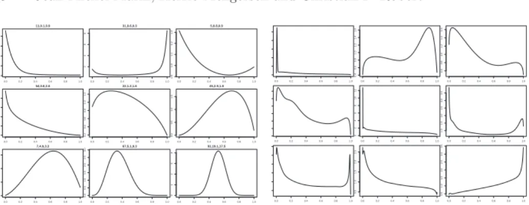
The sum is formally infinite but for obvious practical reasons it needs to be truncated to k ≤ kn, with kn∝ nα, α < 1 (Petrone and Wasserman 2002). Figure 2 represents a few simulations from the Bernstein prior when K is distributed from a Poisson P(λ) distribution and F is the Be(α, β) cdf.
As a final illustration, consider the goodness of fit approach proposed by Robert and Rousseau (2002). The central problem is to test whether or not a given parametric model is compatible with the data at hand. If the null hypothesis holds, the cdf distribution of the sample is U (0, 1). When it does not hold, the cdf can be any cdf on [0, 1]. The choice made in Robert and Rousseau (2002) is to use a general mixture of Beta distributions, (1.6) p0U (0, 1) + (1 − p0)
K X k=1
pkBe(αk, βk) ,
to represent the alternative by singling out the U (0, 1) component, which also is a Be(1, 1) density. Robert and Rousseau (2002) prove the consis-tency of this approximation for a large class of densities on [0, 1], a class that obviously contains the continuous bounded densities already well-approximated by Bernstein polynomials. Given that this is an approxi-mation of the true distribution, the number of components in the mixture is unknown and needs to be estimated. Figure 3 shows a few densities cor-responding to various choices of K and pk, αk, βk. Depending on the range of the (αk, βk)’s, different behaviours can be observed in the vicinities of 0 and 1, with much more variability than with the Bernstein prior which restricts the (αk, βk)’s to be integers.
An alternative to mixtures of Beta distributions for modelling unknown distributions is considered in Perron and Mengersen (2001) in the context of non-parametric regression. Here, mixtures of triangular distributions are used instead and compare favourably with Beta equivalents for certain types of regression, particularly those with sizeable jumps or changepoints.
1.2.4 Reading
Very early references to mixture modelling start with Pearson (1894), even though earlier writings by Quetelet and other 19th century statisticians mention these objects and sometimes try to recover the components. Early (modern) references to mixture modelling include Dempster, Laird and Rubin (1977), who considered maximum likelihood for incomplete data via
0.0 0.2 0.4 0.6 0.8 1.0 0 2 4 6 8 11,0.1,0.9 0.0 0.2 0.4 0.6 0.8 1.0 2 4 6 8 31,0.6,0.3 0.0 0.2 0.4 0.6 0.8 1.0 0.9 1.0 1.1 1.2 1.3 5,0.8,0.9 0.0 0.2 0.4 0.6 0.8 1.0 0 1 2 3 4 54,0.8,2.6 0.0 0.2 0.4 0.6 0.8 1.0 0.2 0.4 0.6 0.8 1.0 1.2 22,1.2,1.6 0.0 0.2 0.4 0.6 0.8 1.0 0.0 0.5 1.0 1.5 45,2.9,1.8 0.0 0.2 0.4 0.6 0.8 1.0 0.0 0.5 1.0 1.5 7,4.9,3.3 0.0 0.2 0.4 0.6 0.8 1.0 0.0 0.5 1.0 1.5 2.0 2.5 3.0 67,5.1,9.3 0.0 0.2 0.4 0.6 0.8 1.0 0 1 2 3 4 91,19.1,17.5
FIGURE 2. Realisations from the Bernstein prior when K ∼ P(λ) and
F is the Be(α, β) cdf for various
val-ues of (λ, α, β). 0.0 0.2 0.4 0.6 0.8 1.0 0 5 10 15 20 25 0.0 0.2 0.4 0.6 0.8 1.0 0.4 0.6 0.8 1.0 1.2 1.4 1.6 0.0 0.2 0.4 0.6 0.8 1.0 0.6 0.8 1.0 1.2 1.4 1.6 0.0 0.2 0.4 0.6 0.8 1.0 0.4 0.6 0.8 1.0 1.2 1.4 1.6 0.0 0.2 0.4 0.6 0.8 1.0 0 2 4 6 8 10 12 0.0 0.2 0.4 0.6 0.8 1.0 1.0 1.5 2.0 2.5 3.0 3.5 0.0 0.2 0.4 0.6 0.8 1.0 0.8 1.0 1.2 1.4 1.6 1.8 0.0 0.2 0.4 0.6 0.8 1.0 0.5 1.0 1.5 2.0 2.5 0.0 0.2 0.4 0.6 0.8 1.0 0.5 1.0 1.5 2.0 2.5 3.0 3.5
FIGURE 3. Some beta mixture den-sities for K = 10 (upper row),
K = 100 (central row) and K = 500 (lower row).
the EM algorithm. In the 1980’s, increasing interest in mixtures included Bayesian analysis of simple mixture models (Bernardo and Giron, 1988), stochastic EM derived for the mixture problem (Celeux and Diebolt, 1985), and approximation of priors by mixtures of natural conjugate priors (Red-ner and Walker, 1984). The 1990’s saw an explosion of publications on the topic, with many papers directly addressing mixture estimation and many more using mixtures of distributions as in, e.g., Kim et al. (1998). Semi-nal texts for finite mixture distributions include Titterington, Smith and Makov (1985), McLachlan and Basford (1987), and McLachlan and Peel (2000).
1.3 The mixture conundrum
If these finite mixture models are so easy to construct and have such widely recognised potential, then why are they not universally adopted? One major obstacle is the difficulty of estimation, which occurs at various levels: the model itself, the prior distribution and the resulting inference.
Example 1
To get a first impression of the complexity of estimating mixture distribu-tions, consider the simple case of a two component normal mixture
(1.7) p N (µ1, 1) + (1 − p) N (µ2, 1)
where the weight p 6= 0.5 is known. The parameter space is then R2 and the
parameters are identifiable: the switching phenomenon presented in Section 1.3.4 does not occur because µ1cannot be confused with µ2when p is known
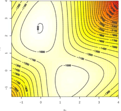
and different from 0.5. Nonetheless, the log-likelihood surface represented in Figure 4 exhibits two modes: one close to the true value of the parameters used to simulate the corresponding dataset and one being a “spurious” mode that does not mean much in terms of the true values of the parameters, but is always present. Obviously, if we plot the likelihood, only one mode is visible because of the difference in the magnitudes.
−1 0 1 2 3 4 −1 0 1 2 3 4 µ1 µ2
FIGURE 4. R image representation of the log-likelihood of the mixture (1.7) for a simulated dataset of 500 observations and true value (µ1, µ2, p) = (0, 2.5, 0.7).
1.3.1 Combinatorics
As noted earlier, the likelihood function (1.4) leads to kn terms when the inner sums are expanded. While this expansion is not necessary to compute the likelihood at a given value¡θ, p¢, which is feasible in O(nk) operations as demonstrated by the representation in Figure 4, the computational dif-ficulty in using the expanded version of (1.4) precludes analytic solutions via maximum likelihood or Bayes estimators (Diebolt and Robert 1990b). Indeed, let us consider the case of n iid observations from model (1.2) and let us denote by π¡θ, p¢the prior distribution on¡θ, p¢. The posterior distribution is then (1.8) π¡θ, p|x¢∝ n Y i=1 k X j=1 pjf (xi|θj) π¡θ, p¢. Example 2
As an illustration of this frustrating combinatoric explosion, consider the case of n observations x = (x1, . . . , xn) from a normal mixture
(1.9) pϕ(x; µ1, σ1) + (1 − p)ϕ(x; µ2, σ2)
under the pseudo-conjugate priors (i = 1, 2)
µi|σi∼ N (ζi, σi2/λi), σ−2i ∼ G a(νi/2, s2i/2), p ∼ Be(α, β) , where G a(ν, s) denotes the Gamma distribution. Note that the hyperparame-ters ζi, σi, νi, si, α and β need to be specified or endowed with an hyperprior when they cannot be specified. In this case θ = ¡µ1, µ2, σ12, σ22
¢ , p = p and the posterior is π (θ, p|x) ∝ n Y j=1 {pϕ(xj; µ1, σ1) + (1 − p)ϕ(xj; µ2, σ2)} π (θ, p) .
This likelihood could be computed at a given value (θ, p) in O(2n) oper-ations. Unfortunately, the computational burden is that there are 2n terms in this sum and it is impossible to give analytical derivations of maximum likelihood and Bayes estimators.
We will now present another decomposition of expression (1.8) which shows that only very few values of the kn terms have a non-negligible influence. Let us consider the auxiliary variables z = (z1, . . . , zn) which
identify to which component the observations x = (x1, . . . , xn) belong.
Moreover, let us denote by Z the set of all knallocation vectors z. The set Z has a rich and interesting structure. In particular, for k labeled components, we can decompose Z into a partition of sets as follows. For a given allocation vector (n1, . . . , nk), where n1+ . . . + nk= n, let us define the set
Zi= ( z : n X i=1 Izi=1= n1, . . . , n X i=1 Izi=k= nk )
which consists of all allocations with the given allocation vector (n1, . . . , nk), relabelled by i ∈ N. The number of nonnegative integer solutions of the de-composition of n into k parts such that n1+ . . . + nk = n is equal to
r = µ n + k − 1 n ¶ .
Thus, we have the partition Z = ∪r
i=1Zi. Although the total number of el-ements of Z is the typically unmanageable kn, the number of partition sets is much more manageable since it is of order nk−1/(k − 1)!. The posterior distribution can be written as
(1.10) π¡θ, p|x¢= r X i=1 X z∈Zi ω (z) π¡θ, p|x, z¢
where ω (z) represents the posterior probability of the given allocation z. Note that with this representation, a Bayes estimator of ¡θ, p¢ could be written as (1.11) r X i=1 X z∈Zi ω (z) Eπ£θ, p|x, z¤
This decomposition makes a lot of sense from an inferential point of view: the Bayes posterior distribution simply considers each possible allocation
z of the dataset, allocates a posterior probability ω (z) to this allocation,
and then constructs a posterior distribution for the parameters conditional on this allocation. Unfortunately, as for the likelihood, the computational burden is that there are knterms in this sum. This is even more frustrating given that the overwhelming majority of the posterior probabilities ω (z) will be close to zero. In a Monte Carlo study, Casella et al. (2000) have showed that the non-negligible weights correspond to very few values of the partition sizes. For instance, the analysis of a dataset with k = 4 components, presented in Example 4 below, leads to the set of allocations with the partition sizes (n1, n2, n3, n4) = (7, 34, 38, 3) with probability 0.59
and (n1, n2, n3, n4) = (7, 30, 27, 18) with probability 0.32, with no other
size group getting a probability above 0.01. Example 1 (continued)
In the special case of model (1.7), if we take the same normal prior on both µ1 and µ2, µ1, µ2 ∼ N (0, 10) , the posterior weight associated with an
allocation z for which l values are attached to the first component, ie such thatPni=1Izi=1= l, will simply be
ω (z) ∝p(l + 1/4)(n − l + 1/4) pl(1 − p)n−l,
because the marginal distribution of x is then independent of z. Thus, when the prior does not discriminate between the two means, the posterior distribution of the allocation z only depends on l and the repartition of the partition size
l simply follows a distribution close to a binomial B(n, p) distribution. If,
instead, we take two different normal priors on the means,
µ1∼ N (0, 4) , µ2∼ N (2, 4) ,
the posterior weight of a given allocation z is now
ω (z) ∝p(l + 1/4)(n − l + 1/4) pl(1 − p)n−l× exp©−[(l + 1/4)ˆs1(z) + l{¯x1(z)}2/4]/2 ª × exp©−[(n − l + 1/4)ˆs2(z) + (n − l){¯x2(z) − 2}2/4]/2 ª
where ¯ x1(z) = 1 l n X i=1 Izi=1xi, x¯2(z) = 1 n − l n X i=1 Izi=2xi ˆ s1(z) = n X i=1 Izi=1(xi− ¯x1(z)) 2 , ˆs2(z) = n X i=1 Izi=2(xi− ¯x2(z)) 2 .
This distribution obviously depends on both z and the dataset. While the computation of the weight of all partitions of size l by a complete listing of the corresponding z’s is impossible when n is large, this weight can be approximated by a Monte Carlo experiment, when drawing the z’s at random. For instance, a sample of 45 points simulated from (1.7) when p = 0.7, µ1= 0 and µ2= 2.5
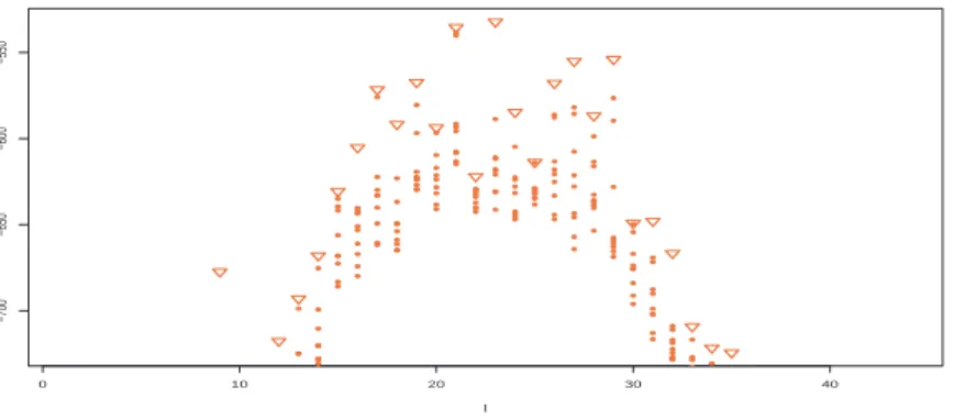
leads to l = 23 as the most likely partition, with a weight approximated by 0.962. Figure 5 gives the repartition of the log ω (z)’s in the cases l = 23 and l = 27. In the latter case, the weight is approximated by 4.56 10−11. (The binomial factor ¡nl¢that corresponds to the actual number of different partitions with l allocations to the first component was taken into account for the approximation of the posterior probability of the partition size.) Note that both distributions of weights are quite concentrated, with only a few weights contributing to the posterior probability of the partition. Figure 6 represents the 10 highest weights associated with each partition size ` and confirms the observation by Casella et al. (2000) that the number of likely partitions is quite limited. Figure 7 shows how observations are allocated to each component in an occurrence where a single5allocation z took all the weight in the simulation
and resulted in a posterior probability of 1.
1.3.2 The EM algorithm
For maximum likelihood computations, it is possible to use numerical op-timisation procedures like the EM algorithm (Dempster et al. 1977), but these may fail to converge to the major mode of the likelihood, as illus-trated below. Note also that, for location-scale problems, it is most often the case that the likelihood is unbounded and therefore the resultant like-lihood estimator is only a local maximum For example, in (1.3), the limit of the likelihood (1.4) is infinite if σ1 goes to 0.
Let us recall here the form of the EM algorithm, for later connections with the Gibbs sampler and other MCMC algorithms. This algorithm is based on the missing data representation introduced in Section 1.2.2, namely that
5Note however that, given this extreme situation, the output of the simulation
experiment must be taken with a pinch of salt: while we simulated a total of about 450, 000 permutations, this is to be compared with a total of 245 permutations
many of which could have a posterior probability at least as large as those found by the simulations.
l=23 log(ω(kt)) −750 −700 −650 −600 −550 0.000 0.005 0.010 0.015 0.020 l=29 log(ω(kt)) −750 −700 −650 −600 −550 0.000 0.005 0.010 0.015 0.020 0.025
FIGURE 5. Comparison of the distribution of the ω (z)’s (up to an additive constant) when l = 23 and when l = 29 for a simulated dataset of 45 observations and true values (µ1, µ2, p) = (0, 2.5, 0.7).
0 10 20 30 40 −700 −650 −600 −550 l
FIGURE 6. Ten highest log-weights ω (z) (up to an additive constant) found in the simulation of random allocations for each partition size l for the same simulated dataset as in Figure 5. (Triangles represent the highest weights.)
−2 −1 0 1 2 3 4 0.0 0.1 0.2 0.3 0.4 0.5
FIGURE 7. Histogram, true components, and most likely allocation found over 440, 000 simulations of z’s for a simulated dataset of 45 observations and true values as in Figure 5. Full dots are associated with observations allocated to the first component and empty dots with observations allocated to the second component.
the distribution of the sample x can be written as f (x|θ) = Z g(x, z|θ) dz = Z f (x|θ) k(z|x, θ) dz (1.12)
leading to a complete (unobserved) log-likelihood Lc(θ|x, z) = L(θ|x) + log k(z|x, θ)
where L is the observed log-likelihood. The EM algorithm is then based on a sequence of completions of the missing variables z based on k(z|x, θ) and of maximisations of the expected complete log-likelihood (in θ):
General EM algorithm
0. Initialization: choose θ(0), 1. Step t. For t = 1, . . . 1.1 The E-step, compute
Q³θ|θ(t−1), x´= E
θ(t−1)[log Lc(θ|x, Z)] ,
where Z ∼ k¡z|θ(t−1), x¢.
1.2 The M-step, maximize Q¡θ|θ(t−1), x¢in θ and take θ(t)= arg max
θ Q
³
θ|θ(t−1), x´.
The result validating the algorithm is that, at each step, the observed L(θ|x) increases.
Example 1 (continued)
For an illustration in our setup, consider again the special mixture of normal distributions (1.7) where all parameters but θ = (µ1, µ2) are known. For a
simulated dataset of 500 observations and true values p = 0.7 and (µ1, µ2) =
(0, 2.5), the log-likelihood is still bimodal and running the EM algorithm on this model means, at iteration t, computing the expected allocations
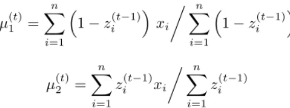
in the E-step and the corresponding posterior means µ(t)1 = n X i=1 ³ 1 − zi(t−1) ´ xi ÁXn i=1 ³ 1 − z(t−1)i ´ µ(t)2 = n X i=1 zi(t−1)xi ÁXn i=1 z(t−1)i
in the M-step. As shown on Figure 8 for five runs of EM with starting points chosen at random, the algorithm always converges to a mode of the likeli-hood but only two out of five sequences are attracted by the higher and more significant mode, while the other three go to the lower spurious mode (even though the likelihood is considerably smaller). This is because the starting points happened to be in the domain of attraction of the lower mode.
−1 0 1 2 3 4 −1 0 1 2 3 4 µ1 µ2
FIGURE 8. Trajectories of five runs of the EM algorithm on the log-likelihood surface, along with R contour representation.
1.3.3 An inverse ill-posed problem
Algorithmically speaking, mixture models belong to the group of inverse
problems, where data provide information on the parameters only
indi-rectly, and, to some extent, to the class of ill-posed problems, where small changes in the data may induce large changes in the results. In fact, when considering a sample of size n from a mixture distribution, there is a non-zero probability (1 − pi)n that the ith component is empty, holding none of the random variables. In other words, there always is a non-zero
proba-bility that the sample brings no information6 about the parameters of one
or more components! This explains why the likelihood function may be-come unbounded and also why improper priors are delicate to use in such settings (see below).
1.3.4 Identifiability
A basic feature of a mixture model is that it is invariant under permutation of the indices of the components. This implies that the component param-eters θi are not identifiable marginally: we cannot distinguish component 1 (or θ1) from component 2 (or θ2) from the likelihood, because they are
ex-changeable. While identifiability is not a strong issue in Bayesian statistics,7
this particular identifiability feature is crucial for both Bayesian inference and computational issues. First, in a k component mixture, the number of modes is of order O(k!) since, if (θ1, . . . , θk) is a local maximum, so is
(θσ(1), . . . , θσ(k)) for every permutation σ ∈ Sn. This makes maximisation and even exploration of the posterior surface obviously harder. Moreover, if an exchangeable prior is used on θ = (θ1, . . . , θk), all the marginals on the
θi’s are identical, which means for instance that the posterior expectation of θ1is identical to the posterior expectation of θ2. Therefore, alternatives
to posterior expectations must be constructed as pertinent estimators. This problem, often called “label switching”, thus requires either a spe-cific prior modelling or a more tailored inferential approach. A na¨ıve answer to the problem found in the early literature is to impose an identifiability
constraint on the parameters, for instance by ordering the means (or the
variances or the weights) in a normal mixture (1.3). From a Bayesian point of view, this amounts to truncating the original prior distribution, going from π¡θ, p¢to
π¡θ, p¢Iµ1≤...≤µk
for instance. While this seems innocuous (because indeed the sampling distribution is the same with or without this indicator function), the in-troduction of an identifiability constraint has severe consequences on the resulting inference, both from a prior and from a computational point of view. When reducing the parameter space to its constrained part, the im-posed trunctation has no reason to respect the topology of either the prior or of the likelihood. Instead of singling out one mode of the posterior, the constrained parameter space may then well include parts of several modes and the resulting posterior mean may for instance lay in a very low proba-bility region, while the high posterior probaproba-bility zones are located at the
6This is not contradictory with the fact that the Fisher information of a
mix-ture model is well defined (Titterington et al. 1985).
7This is because it can be either imposed at the level of the prior distribution
θ(1) −4 −3 −2 −1 0 0.0 0.2 0.4 0.6 0.8 θ(10) −1.0 −0.5 0.0 0.5 1.0 0.0 0.2 0.4 0.6 0.8 1.0 1.2 1.4 θ(19) 1 2 3 4 0.0 0.2 0.4 0.6 0.8
FIGURE 9. Distributions of θ(1), θ(10), and θ(19), compared with the N (0, 1)
prior.
boundaries of this space. In addition, the constraint may radically modify the prior modelling and come close to contradicting the prior information. For instance, Figure 9 gives the marginal distributions of the ordered ran-dom variables θ(1), θ(10), and θ(19), for a N (0, 1) prior on θ1, . . . , θ19. The
comparison of the observed distribution with the original prior N (0, 1) clearly shows the impact of the ordering. For large values of k, the in-troduction of a constraint also has a consequence on posterior inference: with many components, the ordering of components in terms of one of its parameters is unrealistic. Some components will be close in mean while others will be close in variance or in weight. As demonstrated in Celeux et al. (2000), this may lead to very poor estimates of the distribution in the end. One alternative approach to this problem include reparametrisation, as discussed below in Section 1.3.5. Another one is to select one of the k! modal regions of the posterior distribution and do the relabelling in terms of proximity to this region, as in Section 1.4.1.
If the index identifiability problem is solved by imposing an identifiability constraint on the components, most mixture models are identifiable, as described in detail in both Titterington et al. (1985) and MacLachlan and Peel (2000).
1.3.5 Choice of priors
The representation of a mixture model as in (1.2) precludes the use of independent improper priors,
π (θ) =
k Y i=1
since, if Z
πi(θi)dθi= ∞ then for every n, Z
π(θ, p|x)dθdp = ∞
because, among the knterms in the expansion of π(θ, p|x), there are (k−1)n with no observation allocated to the i-th component and thus a conditional posterior π(θi|x, z) equal to the prior πi(θi).
The inability to use improper priors can be seen by some as a marginalia, that is, a fact of little importance, since proper priors with large variances can be used instead.8However, since mixtures are ill-posed problems, this
difficulty with improper priors is more of an issue, given that the influence of a particular proper prior, no matter how large its variance, cannot be truly assessed.
There is still a possibility of using improper priors in mixture models, as demonstrated by Mengersen and Robert (1996), simply by adding some degree of dependence between the components. In fact, it is quite easy to argue against independence in mixture models, because the components are only defined in relation with one another. For the very reason that ex-changeable priors lead to identical marginal posteriors on all components, the relevant priors must contain the information that components are
dif-ferent to some extent and that a mixture modelling is necessary.
The proposal of Mengersen and Robert (1996) is to introduce first a common reference, namely a scale, location, or location-scale parameter. This reference parameter θ0is related to the global size of the problem and
thus can be endowed with a improper prior: informally, this amounts to first standardising the data before estimating the component parameters. These parameters θican then be defined in terms of departure from θ0, as for
instance in θi= θ0+ ϑi. In Mengersen and Robert (1996), the θi’s are more
strongly tied together by the representation of each θi as a perturbation of
θi−1, with the motivation that, if a k component mixture model is used, it is because a (k − 1) component model would not fit, and thus the (k − 1)-th component is not sufficient to absorb 1)-the remaining variability of 1)-the data but must be split into two parts (at least). For instance, in the normal mixture case (1.3), we can consider starting from the N (µ, τ2) distribution,
and creating the two component mixture
pN (µ, τ2) + (1 − p)N (µ + τ θ, τ2$2) .
8This is the stance taken in the Bayesian software winBUGS where improper
If we need a three component mixture, the above is modified into
pN (µ, τ2) + (1 − p)qN (µ + τ ϑ, τ2$21)+
(1 − p)(1 − q)N (µ + τ ϑ + τ σε, τ2$2 1$22).
For a k component mixture, the i-th component parameter will thus be written as
µi= µi−1+ τi−1ϑi= µ + · · · + σi−1ϑi,
σi= σi−1$i= τ · · · $i.
If, notwithstanding the warnings in Section 1.3.4, we choose to impose identifiability constraints on the model, a natural version is to take
1 ≥ $1≥ . . . ≥ $k−1. A possible prior distribution is then
(1.13) π(µ, τ ) = τ−1, p, qj∼ U[0,1], $j ∼ U[0,1], ϑj∼ N (0, ζ2) , where ζ is the only hyperparameter of the model and represents the amount of variation allowed between two components. Obviously, other choices are possible and, in particular, a non-zero mean could be chosen for the prior on the ϑj’s. Figure 10 represents a few mixtures of distributions simulated using this prior with ζ = 10: as k increases, higher order components are more and more concentrated, resulting in the spikes seen in the last rows. The most important point, however, is that, with this representation, we can use an improper prior on (µ, τ ), as proved in Robert and Titterington (1998).
These reparametrisations have been developed for Gaussian mixtures (Roeder and Wasserman 1997), but also for exponential (Gruet et al. 1999) and Poisson mixtures (Robert and Titterington 1998). However, these al-ternative representations do require the artificial identifiability restrictions criticized above, and can be unwieldy and less directly interpretable.9
In the case of mixtures of Beta distributions used for goodness of fit testing mentioned at the end of Section 1.2.3, a specific prior distribution is used by Robert and Rousseau (2002) in order to oppose the uniform component of the mixture (1.6) with the other components. For the uniform weight,
p0∼ Be(0.8, 1.2),
favours small values of p0, since the distribution Be(0.8, 1.2) has an infinite
mode at 0, while pk is represented as (k = 1, . . . , K)
pk =PKωk i=1ωi
, ωk∼ Be(1, k),
9It is actually possible to generalise the U
[0,1]prior on $j by assuming that
either $jor 1/$j are uniform U[0,1], with equal probability. This was tested in
−15 −10 −5 0 0.00 0.10 0.20 −10 −8 −6 −4 −2 0 2 0.00 0.10 0.20 0.30 −2 −1 0 1 2 0.05 0.10 0.15 0.20 0 5 10 15 20 0.0 0.1 0.2 0.3 0 5 10 15 20 0.00 0.10 0.20 0.30 0 5 10 15 20 0.00 0.10 0.20 −2 −1 0 1 2 3 0.0 0.5 1.0 1.5 2.0 −4 −2 0 2 4 0.00 0.10 0.20 −2 0 2 4 6 8 0.0 0.2 0.4 0.6 0.8 1.0 0 5 10 15 0.0 0.2 0.4 0.6 0.8 −8 −6 −4 −2 0 2 0.0 0.4 0.8 1.2 −6 −4 −2 0 2 4 6 0.0 0.2 0.4 0.6 0.8
FIGURE 10. Normal mixtures simulated using the Mengersen and Robert (1996) prior for ζ = 10, µ = 0, τ = 1 and k = 2 (first row), k = 5 (second row), k = 15
(third row) and k = 50 (last row).
for parsimony reasons (so that higher order components are less likely) and the prior (αk, ²k) ∼ ©1 − exp£−θ©(αk− 2)2+ (²k− .5)2ª¤ª × exp£−ζ/{α2 k²k(1 − ²k)} − κα2k/2 ¤ (1.14)
is chosen for the (αk, ²k)’s, where (θ, ζ, κ) are hyperparameters. This form10
is designed to avoid the (α, ²) = (2, 1/2) region for the parameters of the other components.
1.3.6 Loss functions
As noted above, if no identifying constraint is imposed in the prior or on the parameter space, it is impossible to use the standard Bayes estimators on the parameters, since they are identical for all components. As also pointed out, using an identifying constraint has some drawbacks for exploring the parameter space and the posterior distribution, as the constraint may well be at odds with the topology of this distribution. In particular, stochastic exploration algorithms may well be hampered by such constraints if the region of interest happens to be concentrated on boundaries of the con-strained region.
Obviously, once a sample has been produced from the unconstrained pos-terior distribution, for instance by an MCMC sampler (Section 1.4), the ordering constraint can be imposed ex post, that is, after the simulations
10The reader must realise that there is a lot of arbitrariness involved in this
particular choice, which simply reflects the limited amount of prior information available for this problem.
order p1 p2 p3 θ1 θ2 θ3 σ1 σ2 σ3 p 0.231 0.311 0.458 0.321 -0.55 2.28 0.41 0.471 0.303
θ 0.297 0.246 0.457 -1.1 0.83 2.33 0.357 0.543 0.284
σ 0.375 0.331 0.294 1.59 0.083 0.379 0.266 0.34 0.579
true 0.22 0.43 0.35 1.1 2.4 -0.95 0.3 0.2 0.5
TABLE 1.1. Estimates of the parameters of a three component normal mixture, obtained for a simulated sample of 500 points by re-ordering according to one of three constraints, p : p1 < p2 < p3, µ : µ1 < µ2 < µ3, or σ : σ1 < σ2 < σ3.
(Source: Celeux et al. 2000)
have been completed, for estimation purposes (Stephens 1997). Therefore, the simulation hindrance created by the constraint can be completely by-passed. However, the effects of different possible ordering constraints on the
same sample are not innocuous, since they lead to very different
estima-tions. This is not absolutely surprising given the preceding remark on the potential clash between the topology of the posterior surface and the shape of the ordering constraints: computing an average under the constraint may thus produce a value that is unrelated to the modes of the posterior. In addition, imposing a constraint on one and only one of the different types of parameters (weights, locations, scales) may fail to discriminate between
some components of the mixture.
This problem is well-illustrated by Table 1.1 of Celeux et al. (2000). Depending on which order is chosen, the estimators vary widely and, more importantly, so do the corresponding plug-in densities, that is, the densities in which the parameters have been replaced by the estimate of Table 1.1, as shown by Figure 11. While one of the estimations is close to the true density (because it happens to differ widely enough in the means), the two others are missing one of the three modes altogether!
Empirical approaches based on clustering algorithms for the parameter sample are proposed in Stephens (1997) and Celeux et al. (2000), and they achieve some measure of success on the examples for which they have been tested. We rather focus on another approach, also developed in Celeux et al. (2000), which is to call for new Bayes estimators, based on appropriate loss functions.
Indeed, if L((θ, p), (ˆθ, ˆp)) is a loss function for which the labeling is im-material, the corresponding Bayes estimator (ˆθ, ˆp)∗
(1.15) (ˆθ, ˆp)∗= arg min
(ˆθ,ˆp)E(θ,p)|x h
L((θ, p), (ˆθ, ˆp))
i
will not face the same difficulties as the posterior average.
A first loss function for the estimation of the parameters is based on an image representation of the parameter space for one component, like the (p, µ, σ) space for normal mixtures. It is loosely based on the Baddeley ∆
−4 −2 0 2 4 0.0 0.1 0.2 0.3 0.4 0.5 0.6 x y
FIGURE 11. Comparison of the plug-in densities for the estimations of Table 1.1 and of the true density (full line).
metric (Baddeley 1992). The idea is to have a collection of reference points in the parameter space, and, for each of these to calculate the distance to the closest parameter point for both sets of parameters. If t1, . . . , tndenote the collection of reference points, which lie in the same space as the θi’s, and if d(ti, θ) is the distance between tiand the closest of the θi’s, the (L2)
loss function reads as follows: (1.16) L((θ, p), (ˆθ, ˆp)) =
n X i=1
(d(ti, (θ, p)) − d(ti, (ˆθ, ˆp)))2.
That is, for each of the fixed points ti, there is a contribution to the loss if the distance from ti to the nearest θj is not the same as the distance from
ti to the nearest ˆθj.
Clearly the choice of the ti’s plays an important role since we want
L((θ, p), (ˆθ, ˆp)) = 0 only if (θ, p) = (ˆθ, ˆp), and for the loss function to
re-spond appropriately to changes in the two point configurations. In order to avoid the possibility of zero loss between two configurations which actually differ, it must be possible to determine (θ, p) from the {ti} and the
corre-sponding©d(ti, (θ, p)) ª
. For the second desired property, the ti’s are best positioned in high posterior density regions of the (θj, pj)’s space. Given the complexity of the loss function, numerical maximisation techniques like simulated annealing must be used (see Celeux et al. 2000).
When the object of inference is the predictive distribution, more global loss functions can be devised to measure distributional discrepancies. One such possibility is the integrated squared difference
(1.17) L((θ, p), (ˆθ, ˆp)) =
Z R
where f(θ,p) denotes the density of the mixture (1.2). Another possibility
is a symmetrised Kullback-Leibler distance
L((θ, p), (ˆθ, ˆp)) = Z R ½ f(θ,p)(y) log f(θ,p)(y) f(ˆθ,ˆp)(y)
+ f(ˆθ,ˆp)(y) logf(ˆθ,ˆp)(y)
f(θ,p)(y)
¾ dy , (1.18)
as in Mengersen and Robert (1996). We refer again to Celeux et al. (2000) for details on the resolution of the minimisation problem and on the per-formance of both approaches.
1.4 Inference for mixtures models with known
number of components
Mixture models have been at the source of many methodological develop-ments in computational Statistics. Besides the seminal work of Dempster et al. (1977), see Section 1.3.2, we can point out the Data Augmentation method proposed by Tanner and Wong (1987) which appears as a forerun-ner of the Gibbs sampler of Gelfand and Smith (1990). This section covers three Monte Carlo or MCMC (Markov chain Monte Carlo) algorithms that are customarily used for the approximation of posterior distributions in mixture settings, but it first discusses in Section 1.4.1 the solution chosen to overcome the label-switching problem.
1.4.1 Reordering
For the k-component mixture (1.2), with n iid observations x = (x1, . . . , xn),
we assume that the densities f (·|θi) are known up to a parameter θi. In this section, the number of components k is known. (The alternative situation in which k is unknown will be addressed in the next section.)
As detailed in Section 1.3.1, the fact that the expansion of the likelihood (1.2) is of complexity O(kn) prevents an analytical derivation of Bayes estimators: equation (1.11) shows that a posterior expectation is a sum of
kn terms which correspond to the different allocations of the observations
xi and, therefore, is never available in closed form.
Section 1.3.4 discussed the drawbacks of imposing identifiability ordering constraints on the parameter space. We thus consider an unconstrained pa-rameter space, which implies that the posterior distribution has a multiple of k! different modes. To derive proper estimates of the parameters of (1.2), we can thus opt for one of two strategies: either use a loss function as in Section 1.3.6, for which the labeling is immaterial or impose a reordering constraint ex-post, that is, after the simulations have been completed, and
then use a loss function depending on the labeling.
While the first solution is studied in Celeux et al. (2000), we present the alternative here, mostly because the implementation is more straightfor-ward: once the simulation output has been reordered, the posterior mean is approximated by the empirical average. Reordering schemes that do not face the difficulties linked to a forced ordering of the means (or other quan-tities) can be found in Stephens (1997) and Celeux et al. (2000), but we use here a new proposal that is both straightforward and very efficient.
For a permutation τ ∈ Sk, set of all permutations of {1, . . . , k}, we denote by
τ (θ, p) =©(θτ (1), . . . , θτ (k)), (pτ (1), . . . , pτ (k))ª.
the corresponding permutation of the parameter (θ, p) and we implement the following reordering scheme, based on a simulated sample of size M ,
(i) compute the pivot (θ, p)(i∗)
such that
i∗= arg max
i=1,...,Mπ((θ, p)
(i)|x)
that is, a Monte Carlo approximation of the Maximum a Posteriori (MAP) estimator11of (θ, p). (ii) For i ∈ {1, . . . , M }: 1. Compute τi= arg min τ ∈Sk D τ ((θ, p)(i)), (θ, p)(i∗)E 2k
where < ·, · >l denotes the canonical scalar product of Rl 2. Set (θ, p)(i)= τi((θ, p)(i)).
The step (ii) chooses the reordering that is the closest to the approx-imate MAP estimator and thus solves the identifiability problem with-out requiring a preliminary and most likely unnatural ordering on one of the parameters of the model. Then, after the reordering step, the Monte Carlo estimation of the posterior expectation of θi, Eπ
x(θi), is given by PM
j=1(θi)(j) ±
M .
1.4.2 Data augmentation and Gibbs sampling approximations
The Gibbs sampler is the most commonly used approach in Bayesian mix-ture estimation (Diebolt and Robert 1990a, 1994, Lavine and West 1992, Verdinelli and Wasserman 1992, Chib 1995, Escobar and West 1995). Infact, a solution to the computational problem is to take advantage of the missing data introduced in Section 1.2.2, that is, to associate with each observation xj a missing multinomial variable zj ∼ Mk(1; p1, . . . , pk) such
that xj|zj = i ∼ f (x|θi). Note that in heterogeneous populations made of several homogeneous subgroups, it makes sense to interpret zj as the index of the population of origin of xj, which has been lost in the observational process. In the alternative non-parametric perspective, the components of the mixture and even the number k of components in the mixture are of-ten meaningless for the problem to be analysed. However, this distinction between natural and artificial completion is lost to the MCMC sampler, whose goal is simply to provide a Markov chain that converges to the pos-terior distribution. Completion is thus, from a simulation point of view, a means to generate such a chain.
Recall that z = (z1, . . . , zn) and denote by π(p|z, x) the density of the distribution of p given z and x. This distribution is in fact independent of x,
π(p|z, x) = π(p|z). In addition, denote π(θ|z, x) the density of the
distribu-tion of θ given (z, x). The most standard Gibbs sampler for mixture models (1.2) (Diebolt and Robert 1994) is based on the successive simulation of z,
p and θ conditional on one another and on the data: General Gibbs sampling for mixture models
0. Initialization: choose p(0) and θ(0) arbitrarily 1. Step t. For t = 1, . . . 1.1 Generate z(t)i (i = 1, . . . , n) from (j = 1, . . . , k) P ³ zi(t)= j|p(t−1)j , θj(t−1), xi ´ ∝ p(t−1)j f ³ xi|θj(t−1) ´ 1.2 Generate p(t) from π(p|z(t)), 1.3 Generate θ(t) from π(θ|z(t), x).
Given that the density f most often belongs to an exponential family, (1.19) f (x|θ) = h(x) exp(< r(θ), t(x) >k−φ(θ))
where h is a function from R to R+, r and t are functions from Θ and R to
Rk, the simulation of both p and θ is usually straightforward. In this case, a conjugate prior on θ (Robert 2001) is given by
(1.20) π(θ) ∝ exp(< r(θ), α >k−βφ(θ)) ,
where α ∈ Rk and β > 0 are given hyperparameters. For a mixture of distributions (1.19), it is therefore possible to associate with each θj a conjugate prior πj(θj) with hyperparameters αj, βj. We also select for p
the standard Dirichlet conjugate prior, p ∼ D (γ1, . . . , γk). In this case, p|z ∼ D (n1+ γ1, . . . , nk+ γk) and π(θ|z, x) ∝ k Y j=1 exp à < r(θj), α + n X i=1 Izi=jt(xi) >k −φ(θj)(nj+ β) ! where nj = n X l=1
Izl=j. The two steps of the Gibbs sampler are then:
Gibbs sampling for exponential family mixtures 0. Initialization. Choose p(0) and θ(0),
1. Step t. For t = 1, . . . 1.1 Generate zi(t)(i = 1, . . . , n, j = 1, . . . , k) from P ³ zi(t)= j|p(t−1)j , θ(t−1)j , xi ´ ∝ p(t−1)j f ³ xi|θj(t−1) ´ 1.2 Compute n(t)j =Pni=1Iz(t) i =j, s (t) j = Pn i=1Iz(t)i =jt(xi) 1.3 Generate p(t)from D (γ1+ n1, . . . , γ k+ nk), 1.4 Generate θ(t)j (j = 1, . . . , k) from π(θj|z(t), x) ∝ exp ³ < r(θj), α + s(t)j >k−φ(θj)(nj+ β) ´ .
As with all Monte Carlo methods, the performance of the above MCMC algorithms must be evaluated. Here, performance comprises a number of aspects, including the autocorrelation of the simulated chains (since high positive autocorrelation would require longer simulation in order to obtain an equivalent number of independent samples and ‘sticky’ chains will take much longer to explore the target space) and Monte Carlo variance (since high variance reduces the precision of estimates). The integrated autocorre-lation time provides a measure of these aspects. Obviously, the convergence properties of the MCMC algorithm will depend on the choice of distribu-tions, priors and on the quantities of interest. We refer to Mengersen et al. (1999) and Robert and Casella (2004, Chapter 12), for a description of the various convergence diagnostics that can be used in practice.
It is also possible to exploit the latent variable representation (1.5) when evaluating convergence and performance of the MCMC chains for mixtures. As detailed by Robert (1998a), the ‘duality’ of the two chains (z(t)) and
(θ(t)) can be considered in the strong sense of data augmentation (Tanner and Wong 1987, Liu et al. 1994) or in the weaker sense that θ(t) can be
derived from z(t). Thus probabilistic properties of (z(t)) transfer to θ(t). For
instance, since z(t)is a finite state space Markov chain, it is uniformly
geo-metrically ergodic and the Central Limit Theorem also applies for the chain
θ(t). Diebolt and Robert (1993, 1994) termed this the ‘Duality Principle’. In this respect, Diebolt and Robert (1990b) have shown that the na¨ıve MCMC algorithm that employs Gibbs sampling through completion, while appealingly straightforward, does not necessarily enjoy good convergence properties. In fact, the very nature of Gibbs sampling may lead to “trap-ping states”, that is, concentrated local modes that require an enormous number of iterations to escape from. For example, components with a small number of allocated observations and very small variance become so tightly concentrated that there is very little probability of moving observations in or out of them. So, even though the Gibbs chain (z(t), θ(t)) is formally
irreducible and uniformly geometric, as shown by the above duality prin-ciple, there may be no escape from this configuration. At another level, as discussed in Section 1.3.1, Celeux et al. (2000) show that most MCMC samplers, including Gibbs, fail to reproduce the permutation invariance of the posterior distribution, that is, do not visit the k! replications of a given mode.
Example 1 (continued)
For the mixture (1.7), the parameter space is two-dimensional, which means that the posterior surface can be easily plotted. Under a normal prior N (δ, 1/λ) (δ ∈ R and λ > 0 are known hyper-parameters) on both µ1 and µ2, with
sx j =
Pn
i=1Izi=jxi, it is easy to see that µ1 and µ2 are independent, given
(z, x), with conditional distributions
N µ λδ + sx 1 λ + n1 , 1 λ + n1 ¶ and N µ λδ + sx 2 λ + n2 , 1 λ + n2 
respectively. Similarly, the conditional posterior distribution of z given (µ1, µ2)
is easily seen to be a product of Bernoulli rv’s on {1, 2}, with (i = 1, . . . , n) P (zi= 1|µ1, xi) ∝ p exp
³
−0.5 (xi− µ1)2
´
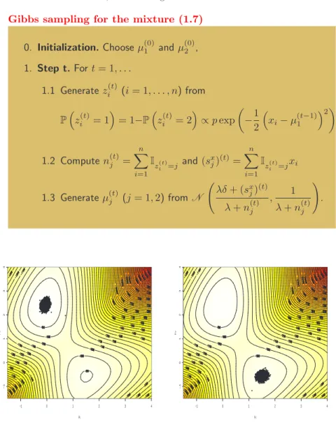
Gibbs sampling for the mixture (1.7) 0. Initialization. Choose µ(0)1 and µ(0)2 , 1. Step t. For t = 1, . . . 1.1 Generate zi(t)(i = 1, . . . , n) from P³zi(t)= 1´= 1−P³zi(t)= 2´∝ p exp µ −1 2 ³ xi− µ(t−1)1 ´2¶ 1.2 Compute n(t)j = n X i=1 Iz(t) i =j and (s x j)(t)= n X i=1 Iz(t) i =jxi 1.3 Generate µ(t)j (j = 1, 2) from N Ã λδ + (sx j)(t) λ + n(t)j , 1 λ + n(t)j ! . −1 0 1 2 3 4 −1 0 1 2 3 4 µ1 µ2
FIGURE 12. Log-posterior surface and the corresponding Gibbs sample for the model (1.7), based on 10, 000 iterations. −1 0 1 2 3 4 −1 0 1 2 3 4 µ1 µ 2
FIGURE 13. Same graph, when ini-tialised close to the second and lower mode, based on 10, 000 iterations.
Figure 12 illustrates the behaviour of this algorithm for a simulated dataset of 500 points from .7N (0, 1) + .3N (2.5, 1). The representation of the Gibbs sample over 10, 000 iterations is quite in agreement with the posterior surface, represented here by grey levels and contours.
This experiment gives a false sense of security about the performances of the Gibbs sampler, however, because it does not indicate the structural de-pendence of the sampler on the initial conditions. Because it uses conditional
distributions, Gibbs sampling is often restricted in the width of its moves. Here, conditioning on z implies that the proposals for (µ1, µ2) are quite concentrated
and do not allow for drastic changes in the allocations at the next step. To obtain a significant modification of z does require a considerable number of iterations once a stable position has been reached. Figure 13 illustrates this phenomenon for the same sample as in Figure 12: a Gibbs sampler initialised close to the spurious second mode (described in Figure 4) is unable to leave it, even after a large number of iterations, for the reason given above. It is quite interesting to see that this Gibbs sampler suffers from the same pathology as the EM algorithm, although this is not surprising given that it is based on the same completion.
This example illustrates quite convincingly that, while the completion is natural from a model point of view (since it is somehow a part of the definition of the model), the utility does not necessarily transfer to the simulation algorithm.
Example 3
Consider a mixture of 3 univariate Poisson distributions, with an iid sample
x from P3j=1pjP(λj), where, thus, θ = (λ1, λ2, λ3) and p = (p1, p2, p3).
Under the prior distribution λj ∼ G a (αj, βj) and p ∼ D (γ1, γ2, γ3) , where
(αj, βj, γj) are known hyperparameters, λj|x, z ∼ G a ¡
αj+ sxj, βj+ nj ¢
and we derive the corresponding Gibbs sampler as follows:
0 5000 10000 15000 20000 7 9 11 13 Iterations λ1 0 5000 10000 15000 20000 0.1 0.3 0.5 Iterations p1 0 5000 10000 15000 20000 2 3 4 5 6 Iterations λ2 0 5000 10000 15000 20000 0.15 0.25 0.35 Iterations p2 0 5000 10000 15000 20000 4 5 6 7 8 Iterations λ3 0 5000 10000 15000 20000 0.1 0.3 0.5 Iterations p3
FIGURE 14. Evolution of the Gibbs chains over 20, 000 iterations for the Poisson mixture model.
Gibbs sampling for a Poisson mixture 0. Initialization. Choose p(0) and θ(0), 1. Step t. For t = 1, . . . 1.1 Generate zi(t)(i = 1, . . . , n) from (j = 1, 2, 3) P ³ z(t)i = j ´ ∝ p(t−1)j ³ λ(t−1)j ´xi exp ³ −λ(t−1)j ´ Compute n(t)j = n X i=1 Iz(t) i =j and (s x j)(t)= n X i=1 Iz(t) i =jxi 1.2 Generate p(t)from D³γ 1+ n(t)1 , γ2+ n(t)2 , γ3+ n(t)3 ´ , 1.3 Generate λ(t)j from G a ³ αj+ (sxj)(t), βj+ n(t)j ´ .
The previous sample scheme has been tested on a simulated dataset with
n = 1000, λ = (2, 6, 10), p1 = 0.25 and p2 = 0.25. Figure 14 presents
the results. We observe that the algorithm reaches very quickly one mode of the posterior distribution but then remains in its vicinity, falling victim of the label-switching effect.
Example 4
This example deals with a benchmark of mixture estimation, the galaxy dataset of Roeder (1992), also analyzed in Richardson and Green (1997) and Roeder and Wasserman (1997), among others. It consists of 82 observations of galaxy velocities. All authors consider that the galaxies velocities are reali-sations of iid random variables distributed according to a mixture of k normal distributions. The evaluation of the number k of components for this dataset is quite delicate,12 since the estimates range from 3 for Roeder and Wasserman
(1997) to 5 or 6 for Richardson and Green (1997) and to 7 for Escobar and West (1995), Phillips and Smith (1996). For illustration purposes, we follow Roeder and Wasserman (1997) and consider 3 components, thus modelling the data by 3 X j=1 pjN ¡ µj, σ2j ¢ .
12In a talk at the 2000 ICMS Workshop on mixtures, Edinburgh, Radford Neal
presented convincing evidence that, from a purely astrophysical point of view, the number of components was at least 7. He also argued against the use of a mixture representation for this dataset!
In this case, θ = (µ1, µ2, µ3, σ21, σ23, σ32). As in Casella et al. (2000), we use conjugate priors σ2j ∼ I G (αj, βi) , µj|σj2∼ N ¡ λj, σj2/τj ¢ , (p1, p2, p3) ∼ D (γ1, γ2, γ3) ,
where I G denotes the inverse gamma distribution and ηj, τj, αj, βj, γj are known hyperparameters. If we denote
svj = n X i=1 Izi=j(xi− µj) 2, then µj|σj2, x, z ∼ N Ã λjτj+ sxj τj+ nj , σ2 j τj+ nj ! , σ2j|µj, x, z ∼ I G ¡ αj+ 0.5(nj+ 1), βj+ 0.5τj(µj− λj)2+ 0.5svj ¢ . Gibbs sampling for a Gaussian mixture
0. Initialization. Choose p(0), θ(0), 1. Step t. For t = 1, . . . 1.1 Generate z(t)i (i = 1, . . . , n) from (j = 1, 2, 3) P ³ zi(t)= j ´ ∝ p (t−1) j σj(t−1)exp µ − ³ xi− µ(t−1)j ´2 /2¡σj2 ¢(t−1)¶ Compute n(t)j = n X l=1 Iz(t) l =j, (s x j)(t)= n X l=1 Iz(t) l =jxl 1.2 Generate p(t) from D (γ1+ n1, γ 2+ n2, γ3+ n3) 1.3 Generate µ(t)j from N Ã λjτj+ (sxj)(t) τj+ n(t)j , ¡ σ2 j ¢(t−1) τj+ n(t)j ! Compute¡svj ¢(t) = n X l=1 Iz(t) l =j ³ xl− µ(t)j ´2 1.4 Generate¡σ2 j ¢(t) (j = 1, 2, 3) from I G µ αj+nj+ 1 2 , βj+ 0.5τj ³ µ(t)j − λj ´2 + 0.5¡svj ¢(t)¶ .