DOCTORAT DE L'UNIVERSITÉ DE TOULOUSE
Délivré par :
Institut National Polytechnique de Toulouse (INP Toulouse)
Discipline ou spécialité :
Réseaux, Télécommunications, Systèmes et Architecture
Présentée et soutenue par :
M. FLORIAN RIBAUD
le lundi 5 décembre 2016
Titre :
Unité de recherche :
Ecole doctorale :
Analysis of Multipath Channel Reduction Models for the Testing of Realistic
GNSS Receivers
Mathématiques, Informatique, Télécommunications de Toulouse (MITT)
Département d'Ingénierie de Systèmes Complexes (DISC-ISAE)
Directeur(s) de Thèse :
M. OLIVIER JULIEN M. FERNANDO PEREZ FONTAN
Rapporteurs :
M. CLAUDE OESTGES, UNIVERSITE CATHOLIQUE DE LOUVAIN M. TERRY MOORE, THE UNIVERSITY OF NOTTINGHAM GB
Membre(s) du jury :
1 M. CLAUDE OESTGES, UNIVERSITE CATHOLIQUE DE LOUVAIN, Président
2 M. FERNANDO PEREZ FONTAN, UNIVERSIDAD DE VIGO, Membre
2 M. OLIVIER JULIEN, ECOLE NATIONALE DE L'AVIATION CIVILE, Membre
Florian RIBAUD – PhD thesis Page 3 Bien des personnes ont joué des rôles importants durant les trois dernières années que je viens de passer en tant que doctorant de l’ONERA, au service DEMR. Dans un premier, il faudra remercier toutes les personnes impliquées de près ou de loin dans la rédaction du présent manuscrit et dans le travail de thèse qu’il contient. Egalement, le support moral assuré par nombre de personnes de mon entourage devra être gratifié.
Dans un premier temps, j’aimerais remercier toute l’unité RCP du service, pour son accueil et son environnement de travail cent pour cent compatible avec la recherche, à travers M. Laurent Castanet (chef de l’unité RCP) et M. Florent Christophe (directeur du service DEMR). J’aimerais également accorder une mention spéciale à Mme Corinne De Pablo, secrétaire du service DEMR, dont les compétences et la patience m’ont soustrait à bien de misères administratives. Enfin, je ne dois pas oublier de citer Xavier Boulanger, qui a accepté de recueillir un doctorant dans son bureau dès le début de ma thèse, et durant les trois années suivantes dans une ambiance très agréable.
En ce qui concerne le travail de thèse, il est très important de remercier toute mon équipe d’encadrement, à commencer par mon directeur de thèse M. Olivier Julien de l’ENAC pour ses précieuses recommandations techniques ou administratives. Egalement, je remercie M. Joël Lemorton, mon encadrant ONERA, pour sa patience et ses conseils durant les trois années. Sans oublier mon co-directeur de thèse, M. Fernando Perez-Fontan de l’université de Vigo, avec qui il a été très agréable de travailler durant ses séjours à Toulouse.
Enfin, c’est à Mehdi Ait-Ighil et à Sébastien Rougerie que je dois l’aide la plus précieuse. Mehdi a pris part à l’encadrement de la thèse en tant que spécialiste du simulateur SCHUN (qu’il a lui-même implémenté). Sans ses conseils très avisés et sa patience tout au long des trois ans, cette thèse n’aurait peut-être jamais vu le jour. Sébastien a joué son rôle d’encadrant côté CNES à merveille, et bien plus encore. Je dois le remercier particulièrement pour ses indications concernant l’algorithme d’optimisation SAGE. Egalement, je remercie Mehdi et Sébastien pour la patience qu’ils ont mise dans la relecture de mon manuscrit. Il me faut également remercier M. Frédéric Lacoste (CNES) pour l’encadrement de la première année, et de m’avoir donné l’idée et l’envie de me lancer dans une thèse durant mon PFE effectué au CNES.
J’ai bénéficié d’un soutien moral considérable de la part de mes collègues doctorants, en particulier ceux qui m’ont aidé à rythmer les activités extra-professionnelles, à coups de matchs de foot, bars et paillotes (le week-end et pas seulement …). Les vrais se reconnaitront. Enfin, qu’auraient été ces trois ans sans mes fidèles colocs, qui ont partagé la vie de tous les jours d’un thésard. Grâce à Geoffrey C., Ghislain R., Jean-Elie D. et Hugo J., les bons comme les mauvais moments étaient toujours festifs. Merci bien sûr à tous nos amis qui ont partagé ces longues soirées, que je ne citerai pas de peur d’oublier quelqu’un.
Enfin, merci à mes parents, pour leur soutien permanant durant mes études. Merci également à mes frères, en particulier ceux qui se sont déplacés pour assister à ma soutenance.
Merci infiniment à tous !! Allez le RC Strasbourg ! Florian
Introduction ... 18
1. Modeling of the LMS channel and introduction to the problem of channel reduction ... 22
1.1. Different approaches to model the LMS channel ... 23
1.1.1. Statistical approaches... 23
1.1.1.1. The narrow-band statistical models ... 23
1.1.1.2. The state oriented statistical models ... 25
1.1.1.3. The wide-band statistical models ... 26
1.1.1.4. Synthesis on the statistical channel models ... 27
1.1.2. Deterministic channel models ... 27
1.1.2.1. General principle ... 27
1.1.2.2. The full-wave methods ... 28
1.1.2.3. The asymptotic methods ... 28
1.1.2.4. Presentation of the SE RAY-EM Fermat software ... 29
1.1.2.5. Synthesis on the deterministic channel models ... 30
1.1.3. Hybrid channel models ... 30
1.1.3.1. Narrow-band hybrid models ... 30
1.1.3.2. Wide-band hybrid models ... 31
1.1.3.3. Synthesis on the hybrid models ... 32
1.2. The SCHUN simulator ... 32
1.2.1. General presentation of the simulator ... 33
1.2.2. Architecture of the model ... 33
1.2.3. The statistical module: the virtual city ... 34
1.2.4. The deterministic module ... 36
1.2.4.1. The coherent contribution ... 36
1.2.4.2. The multipath ... 37
1.3. Validation of the SCHUN simulator and introduction to the channel reduction problem ... 42
1.3.1. Validation of the SCHUN simulator ... 42
1.3.2. The channel reduction problem ... 44
1.4. Conclusion ... 46
2. Implementation of an optimal method to reduce the channel impulse response by aggregating or selecting multipaths ... 48
Florian RIBAUD – PhD thesis Page 6
2.2.1. Presentation of the reference scenario ... 50
2.2.2. Computation of the impulse response ... 51
2.2.2.1. Power--delay spread of the impulse response ... 51
2.2.2.2. Doppler spectrogram of the impulse response ... 53
2.3. Preliminary test: performance of the selection methods ... 54
2.3.1. Literature overview ... 54
2.3.2. Implementation and assessment of the selection methods ... 55
2.4. Tap Delay Line channel models ... 58
2.4.1. Literature overview ... 58
2.4.2. Tap Delay Line approach ... 59
2.4.3. Channel re-sampling techniques ... 63
2.4.4. Doppler spectrum of the reduced channels ... 69
2.4.5. Conclusion of the Tap Delay Line study ... 73
2.5. Channel clustering techniques ... 73
2.5.1. Literature overview ... 73
2.5.2. Multipath distance ... 74
2.5.3. Reduction of the impulse response using the Single Linkage Approach ... 76
2.5.3.1. General presentation of the Single Linkage Clustering ... 76
2.5.3.2. Application to the channel impulse response reduction and results ... 78
2.5.3.3. Complexity of the Single Linkage technique ... 81
2.5.4. Reduction of the impulse response using the K-Means clustering algorithm ... 82
2.5.4.1. General presentation of the K-Means clustering algorithm ... 82
2.5.4.2. Application to the channel impulse response reduction and results ... 83
2.5.5. Enhancement of the K-Means algorithm by weighting the clusters ... 88
2.5.5.1. Presentation of the Soft K-Means ... 88
2.5.5.2. Adaptation of the Soft K-Means to the multipath impulse response ... 89
2.5.5.3. Application of the Soft K-Means clustering to the reference channel ... 90
2.5.5.4. Continuity of the multipaths ... 92
2.6. Conclusion ... 94
3. Implementation of a parametric optimization method to preserve the channel autocorrelation function ... 96
Florian RIBAUD – PhD thesis Page 7
3.2. Adaptation and application of the SAGE algorithm to the cost function ... 98
3.2.1. Definition of the cost function ... 98
3.2.2. Resolution of the optimization problem using the SAGE algorithm ... 100
3.2.2.1. Presentation of SAGE and hypothesis ... 100
3.2.2.2. Implementation of SAGE ... 101
3.2.2.3. Influence of the parameters of the algorithm ... 105
3.3. Validation of SAGE and limitations ... 106
3.3.1. Implementation of the canonical scenario ... 106
3.3.2. Impact of the Doppler resolution on the power-delay and Doppler spectrogram ... 107
3.3.3. Preservation of the channel autocorrelation function ... 111
3.3.4. Synthesis ... 112
3.4. Reduction of the reference impulse response using SAGE ... 113
3.4.1. Assessment of the delay and Doppler preservation ... 113
3.4.2. Influence of the number of echoes on the channel characteristics preservation ... 116
3.5. Complexity of the algorithm ... 117
3.6. Conclusion ... 118
4. Reduction of the multipath channel using a Markov process ... 120
4.1. Introduction of the problem and literature overview ... 121
4.2. Description of the CRIME algorithm and adaptation to the channel reduction problem ... 121
4.2.1. Data formatting ... 122
4.2.2. Implementation of the CRIME algorithm ... 122
4.2.2.1. Architecture of CRIME ... 122
4.2.2.2. Estimation of the parameters of the reduced channel ... 124
4.2.2.3. Drawing of the multipath parameters from the pdfs ... 132
4.3. Application of CRIME to the reference scenario ... 134
4.3.1. Evolution of the delay and amplitude parameters ... 134
4.3.1.1. Delays ... 134
4.3.1.2. Amplitudes ... 135
4.3.1.3. Synthesis ... 136
Florian RIBAUD – PhD thesis Page 8
4.4. Modification of CRIME and application to the reference impulse response ... 141
4.4.1. Modification of CRIME ... 141
4.4.2. Application of the modified version of CRIME to the reference scenario ... 145
4.5. Conclusion ... 147
5. Comparison of the reduction methods according to the pseudo-range error preservation .... 149
5.1. Introduction of the study and literature overview ... 150
5.1.1. Methods to compare ... 150
5.1.2. Literature overview ... 150
5.2. Implementation of the reference scenario ... 152
5.2.1. Definition of the environment ... 152
5.2.2. Channel sampling frequency ... 153
5.3. Open loop discriminator error conservation ... 154
5.3.1. Open loop discriminator error estimation ... 154
5.3.2. Discriminator error for the different angles of arrival ... 156
5.3.3. Comparison of the reduction methods according to the open loop discriminator error preservation ... 157
5.3.4. Influence of the number of multipaths in the reduced channel ... 161
5.3.5. Synthesis on the preservation of the open loop discriminator error ... 163
5.4. Tracking error conservation ... 163
5.4.1. Presentation of the GeneIQ software receiver ... 163
5.4.2. Tracking error for the different angles of arrival ... 164
5.4.3. Comparison of the reduction methods according to the tracking error preservation ... 166
5.4.4. Influence of the number of multipaths in the reduced channel ... 169
5.4.5. Synthesis on the preservation of the tracking error ... 170
5.5. Influence of the parameters of the GNSS simulation on the comparison ... 171
5.5.1. Influence of the RF bandwidth ... 171
5.5.2. Influence of the noise ... 173
Florian RIBAUD – PhD thesis Page 9
Conclusion ... 184
A. Annex A: Proposition of a method to follow the signature of the multipaths along consecutive impulse response samples ... 187
A.1. Introduction of the problematic ... 187
A.2. Presentation of the algorithm ... 188
A.3. Results of the algorithm ... 190
B. Annex B: Demonstration of the discriminator error open loop close formula ... 191
B.1. Definition of the discriminator open loop error ... 191
B.2. Development of the formula ... 192
B.2.1. Hypothesis: ... 192
B.2.2. Calculation and result ... 194
B.3. Validation of the formula ... 195
Introduction en français ... 198
Conclusion en français ... 202
Abstract ... 205
Résumé ... 208
Florian RIBAUD – PhD thesis Page 10
List of Figures
Figure 1.1 : Illustration of the shadowing and fast fading effects on the narrow-band power ... 23
Figure 1.2 : Illustration of a 2-states Markov chain ... 25
Figure 1.3 : Illustration of the PO, ECM and GO coupling in the SE-RAY-FERMAT module... 29
Figure 1.4 : Architecture of SCHUN, with statistical and deterministic components ... 33
Figure 1.5 : Illustration of an urban canyon ... 35
Figure 1.6 : Illustration of two urban canyons with 75% (left) and 25% (right) building density ... 35
Figure 1.7 : Three examples of building façades ... 35
Figure 1.8 : Illustration of the LOS/NLOS and UTD models for direct path blockage ... 37
Figure 1.9 : Density function of the scatterers positions from the measurements of [Lehn 08] ... 37
Figure 1.10 : Schematization of the 3CM in [Ait 13] ... 38
Figure 1.11 : RCS of a perfect dielectric plate using the 3CM specular model [Ait 13] ... 39
Figure 1.12 : Dimensioning and positioning of the equivalent plate to model the backscattering component of the 3CM ... 40
Figure 1.13 : RCS of a backscattering echo using the 3CM model [Ait 13] ... 40
Figure 1.14 : RCS corresponding to the different slightly rough surface models... 41
Figure 1.15 : RCS of the incoherent scattering echo considering a very rough facet with Gaussian and exponential distributions [Ait 13] ... 41
Figure 1.16 : Validation of the 3CM model on a single canonical façade ... 42
Figure 1.17 : Validation of the UTD model with the SCHUN simulator ... 43
Figure 1.18 : Number of multipaths in the impulse response along the receiver's trajectory ... 45
Figure 1.19 : Duration of the tracking error computation along the 1 km trajectory using GeneIQ .... 45
Figure 1.20 : Overview of the NAVYS constellation simulator ... 46
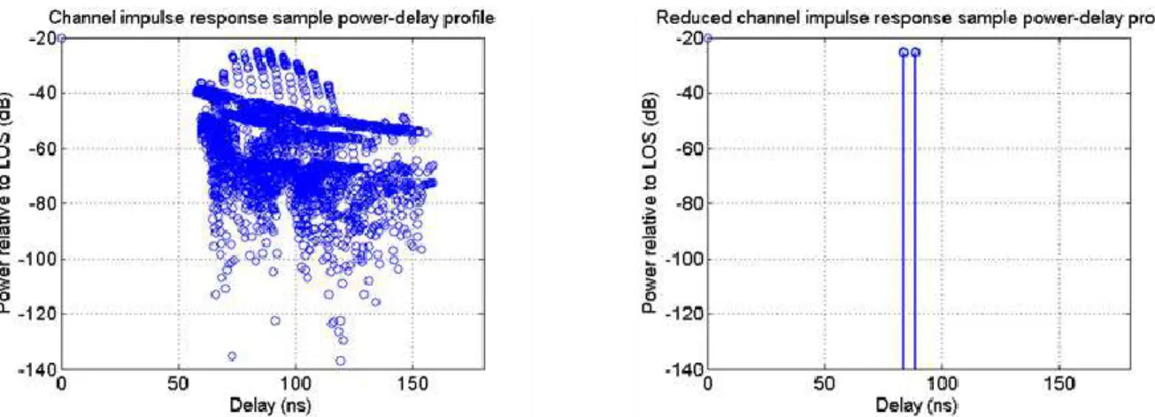
Figure 2.1 : Example of channel impulse response power in terms of delay, Doppler and angle of arrival ... 49
Figure 2.2 : Example of channel impulse response power-Delay and Doppler-Delay profile ... 50
Figure 2.3: Virtual city of the reference scenario and emitter-receiver configuration ... 51
Figure 2.4: Illustration of the reference scenario virtual city façades ... 51
Figure 2.5: Evolution of the power-delay spread along the trajectory ... 52
Figure 2.6: Doppler spectrogram of the multipath channel along the trajectory of the reference scenario ... 54
Figure 2.7: Illustration of impulse response reduction using the minimum energy error selection method at distance d=25 m of the reference scenario ... 55
Figure 2.8: Zoom on the reduced channel impulse response of Fig. 2.7 ... 55
Figure 2.9: Comparison of the reference channel impulse response power in terms of angle of arrival with the selection method reduced one ... 56
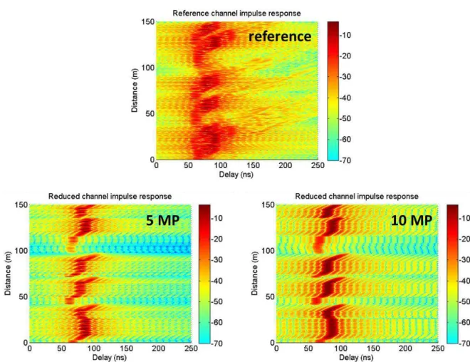
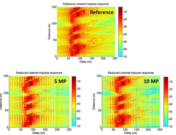
Florian RIBAUD – PhD thesis Page 11 Figure 2.10: Reduced power-Delay profile along the trajectory with 5 and 10 contributions in the
reduced channel (bottom) compared with the reference channel (on top) ... 56
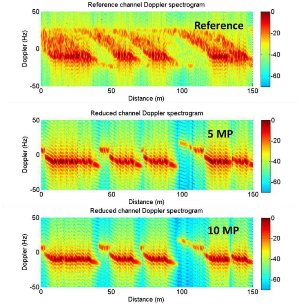
Figure 2.11: Reduced channel Doppler spectrogram along the trajectory with 5 and 10 contributions in the reduced channel ... 57
Figure 2.12: Illustration of the delay line scaling process ... 59
Figure 2.13: Illustration of the Tap Delay Line reduction effect on the power-delay profile at time t=5s, with ∆𝝉=20 ns tap width ... 60
Figure 2.14: Evolution of the multipath delays and power (color) along the [12 m, 50 m] segment of the reference scenario with ∆𝝉=40 ns tap width ... 60
Figure 2.15: Illustration of the Tap Delay Line reduction process... 61
Figure 2.16: Comparison of the reduced channel impulse responses (bottom) with the reference (on top) for 5 and 10 multipaths using the Tap Delay Line ... 62
Figure 2.17: Illustration of the continuous channel construction ... 64
Figure 2.18: Illustration of the continuous channel sampling process ... 64
Figure 2.19: Example of channel transfer function, at t=5 s on the reference scenario ... 65
Figure 2.20: Example of reduce channel Power-Delay profile at time t=5s ... 67
Figure 2.21: Example of T=transfer function comparison at time t=5s... 68
Figure 2.22: Evolution of the Power-delay profile along the trajectory with 5 and 10 multipaths in the re-sampled channel ... 68
Figure 2.23: Comparison of the Tap Delay Line reduced channel (left plot) and resampled channel (right plot) transfer function with the reference transfer function at time t=10 s ... 69
Figure 2.24: Comparison of the reference channel Doppler spectrum (top plot) with the re-sampled channel Doppler spectrum along the trajectory ... 70
Figure 2.25: Comparison of the reference channel Doppler spectrum (top plot) with the Tap Delay Line reduced channel Doppler spectrum along the trajectory ... 71
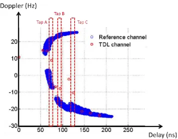
Figure 2.26: Illustration of the Doppler diversity of the multipaths in three taps of the reference Doppler-delay profile ... 72
Figure 2.27: Illustration of the Single Linkage clustering performance ... 78
Figure 2.28: Illustration of the Single Linkage reduced channel with 5 and 10 multipath at time t=6 s on the reference scenario ... 79
Figure 2.29: Comparison of the reference scenario impulse response with the Single Linkage reduced ones with 5 and 10 clusters, at t=6 s ... 79
Figure 2.30: Comparison of the reference scenario impulse response with the Tap Delay Line reduced ones with 5 and 10 clusters, at t=6 s ... 80
Figure 2.31: Comparison of the reference scenario Doppler spectrum with the Single Linkage reduced ones with 5 and 10 clusters, at time t=25 s ... 81
Figure 2.32: Illustration of the K-Means reduced channel with 5 (left) and 10 (right) multipaths at time t=6 s ... 84
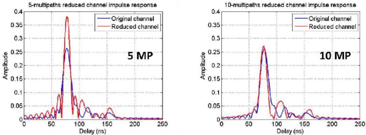
Figure 2.33: Evolution of the Power-delay profile of the reference channel (top plot) and clustering reduced ones along the receiver's trajectory... 85
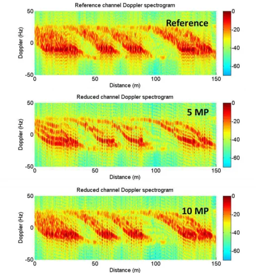
Florian RIBAUD – PhD thesis Page 12 Figure 2.34: Comparison of the reference channel Doppler spectrogram (top plot) with 5- and
10-multipath reduced channel Doppler spectrogram along the trajectory ... 86
Figure 2.35: Evolution of the Power-delay profile of the reference channel (top plot) and Soft K-Means reduced ones along the trajectory ... 90
Figure 2.36: Comparison of the reference channel Doppler spectrum (top plot) with the 5- and 10-multipath reduced channel Doppler spectra along the trajectory ... 91
Figure 2.37: Delay evolution of the reduced channel multipaths with the Hard and Soft K-Means algorithms on the [75m-100m] segment ... 92
Figure 2.38: Doppler evolution with the Hard and Soft K-Means algorithms on [75m-100m] ... 93
Figure 2.39: Delay evolution of the reduced channel multipaths with the Hard and Soft K-Means algorithms on the [125m-150m] segment ... 94
Figure 2.40: Doppler evolution of the reduced channel multipaths with the Hard and Soft K-Means algorithms on the [125m-150m] segment ... 94
Figure 3.1 : Illustration of the SAGE algorithm architecture ... 104
Figure 3.2: Illustration of the canonical scenario with two multipath sources ... 106
Figure 3.3: Original channel impulse response with 2 multipath sources ... 107
Figure 3.4: Original channel Doppler spectrogram ... 107
Figure 3.5: Impulse response power-delay profile of the reduced channel for different numbers of multipath and different Doppler resolutions of SAGE ... 108
Figure 3.6: Impulse response power-delay profile of the reduced channel for different numbers of multipath and different Doppler resolutions of SAGE ... 109
Figure 3.6: Doppler evolution of MP1 and MP2 ... 109
Figure 3.7: Delay evolution of the 2 paths estimated by SAGE with 20 Hz Doppler resolution ... 110
Figure 3.9: Examples of autocorrelation functions comparison corresponding to the original and estimated channels ... 112
Figure 3.10: Comparison between the reference channel (on the left) and the SAGE reduced channel (on the right) power-delay profiles ... 114
Figure 3.11: Comparison of the estimated channel impulse response with the reference ... 114
Figure 3.12: Evolution of the delay of the first estimated multipath ... 115
Figure 3.13: Evolution of the reference (on top) and estimated multipath channels (bottom) Doppler spectrograms ... 115
Figure 3.14: Power-delay profile of the estimated channel for 2, 5 and 10 multipaths in the reduced channel ... 116
Figure 4.1 : Principle of CRIME scheme ... 124
Figure 4.2: Markov chain of the reduced channel delays with K delay states/bins ... 124
Figure 4.3: Delay pdf at the times t=0 s, t=10 s, t=20 s, t=30 s on the reference scenario ... 125
Figure 4.4: Evolution of the delay of 3 multipaths of the original channel on the [50 m, 60 m] segment ... 126
Florian RIBAUD – PhD thesis Page 13 Figure 4.6: Density function of 𝑃(𝜏(𝑡𝑖)|𝜏(𝑡𝑖−1) ∈ 𝑇𝑎) on the left and 𝑃(𝜏(𝑡𝑖)|𝜏(𝑡𝑖−1) ∈ 𝑇𝑏) on the
right ... 127
Figure 4.7: Markov chain of the reduced channel amplitudes with the delay dependency with 𝐾 amplitude states ... 128
Figure 4.8: Power pdf at the times t=0 s, t=10 s, t=20 s, t=30 s on the reference scenario... 129
Figure 4.9: Power delay profile of the impulse response at the time t=20 s ... 130
Figure 4.10: Density function of 𝑃(𝛾(𝑡𝑖+1)|𝛾(𝑡𝑖) ∈ 𝐴𝑎) (left) and 𝑃(𝛾(𝑡𝑖+1)|𝛾(𝑡𝑖) ∈ 𝐴𝑏) (right) ... 130
Figure 4.11: Density function of 𝑃(𝛾(𝑡𝑖+1)|𝜏(𝑡𝑖) ∈ 𝑇𝑎) (left) and 𝑃(𝛾(𝑡𝑖+1)|𝜏(𝑡𝑖) ∈ 𝑇𝑏) (right) ... 131
Figure 4.12: Density function associated to 𝑃(𝛾(𝑡𝑖+1)|𝜏(𝑡𝑖∈ 𝑇𝑎 ∩ 𝛾(𝑡𝑖) ∈ 𝐴𝑎) (left) and 𝑃(𝛾(𝑡𝑖+1)|𝜏(𝑡𝑖 ∈ 𝑇𝑏 ∩ 𝛾(𝑡𝑖) ∈ 𝐴𝑏) (right) ... 131
Figure 4.13: Cumulative density function of 𝑃(𝜏(𝑡𝑖)|𝜏(𝑡𝑖−1) ∈ 𝑇𝑎) on the left and 𝑃(𝜏(𝑡𝑖)|𝜏(𝑡𝑖−1) ∈ 𝑇𝑏) on the right ... 132
Figure 4.14: Cumulative density function associated to 𝑃(𝛾(𝑡𝑖+1)|𝜏(𝑡𝑖∈ 𝑇𝑎 ∩ 𝛾(𝑡𝑖) ∈ 𝐴𝑎)(left) and 𝑃(𝛾(𝑡𝑖+1)|𝜏(𝑡𝑖 ∈ 𝑇𝑏 ∩ 𝛾(𝑡𝑖) ∈ 𝐴𝑏) (right) ... 133
Figure 4.15: Delay evolution of the reduced channel multipaths of 4 realizations of the CRIME process along the [75m,100m] segment of the trajectory ... 135
Figure 4.16: Power evolution of the reduced channel multipaths of 4 realizations of the CRIME process along the [75 m,100 m] segment of the trajectory... 136
Figure 4.17: Power-delay profile of the reference channel (left) and the CRIME reduced channel (right) ... 137
Figure 4.18: Power-delay profile (left) and power-Doppler profile (right) at t=5 s ... 138
Figure 4.19: Density function of the delays and impulse response power-delay profile at t=5 s ... 138
Figure 4.20: Density function of the delays and impulse response power-delay profile at t=25 s ... 139
Figure 4.21: Density function of the amplitudes of the multipaths whose delay is tapped into the frame of the left plot at t=5 s ... 140
Figure 4.22: Density function of the amplitudes of the multipaths whose delay is tapped into the frame of the left plot at t=15 s ... 140
Figure 4.23: New version of the density function of the delay distribution (left) and impulse response power-delay profile at t=25 s ... 143
Figure 4.24: Illustration of the complex amplitude estimation process at t=25 s ... 144
Figure 4.25: Principle of the modified version of CRIME ... 145
Figure 4.26: Illustration of the impulse response power-delay profile for the original (left) and reduced (right) channels along the trajectory using the new statistic method ... 145
Figure 4.27: Illustration of the Doppler spectrogram of the original (above) and reduced (below) channels along the trajectory using the new statistic method ... 146
Figure 5.1: Illustration of the reference scenario ... 152
Figure 5.2: Autocorrelation function of the channel (on the left) and coherency time in terms of elevation and azimuth of the incoming signal ... 153
Figure 5.3: Illustration of an autocorrelation function distortion by a multipath channel and of the resulting S-curve ... 155
Florian RIBAUD – PhD thesis Page 14 Figure 5.4: Discriminator error along the [250m,500m] of the trajectory for different angles of
arrival ... 156
Figure 5.5: Cumulative distribution of the difference between the reference and reduced channel discriminator errors for different emitter azimuths 𝛼 and elevations 𝛽 ... 159
Figure 5.6: Time series of the difference between original and reduced discriminator open loop errors for 𝛼 = 30°,𝛽 = 35° ... 160
Figure 5.7: Reference channel discriminator error with highlight on the 5% largest difference samples ... 161
Figure 5.8: Cumulative distribution of the difference between the reference and reduced channel discriminator errors for different numbers of multipaths in the reduced channel ... 162
Figure 5.9: Tracking error of the receiver all along the trajectory for the different angles of arrival 165 Figure 5.10: Cumulative distribution of the difference between the reference and reduced channel tracking errors for different emitter azimuths α and elevations 𝛽 ... 167
Figure 5.11 : Cumulative distribution of the difference between the reference and reduced channel tracking errors for different numbers of multipaths in the reduced channel ... 169
Figure 5.12: Cumulative distributions of the tracking error difference between original and reduced channels for different RF bandwidths ... 172
Figure 5.13: Tracking error of the original channel with (ON) and without (OFF) noise on the segment [250m, 500m] ... 174
Figure 5.14: Cumulative distributions of the tracking error difference between original and reduced channels with noise (ON) and without (OFF) noise ... 174
Figure 5.15: Cumulative distributions of the tracking error difference between original and reduced channels considering BPSK (left) and BOC (right) modulated signals ... 176
Figure 5.16 : Mean difference between original and reduced channel discriminator error for different azimuths and elevations ... 178
Figure 5.17: 95% discriminator error preservation of the reduction methods for different azimuths and elevations ... 178
Figure 5.18: 99% discriminator error preservation of the reduction methods for different azimuths and elevations ... 178
Figure 5.19: Influence of the elevation on the power-delay profile conservation at d= 125 m ... 180
Figure 5.20: Influence of the elevation on the multipath delay at d= 125 m ... 181
Figure 5.21: Influence of the azimuth on the delay spread at d= 500 m ... 181
Figure A.1 : Illustration of a 2-dimensional pdf ... 187
Figure A.2 : Reference scenario ... 188
Figure A.3 : Variation of the Doppler of source B considering three elevations ... 189
Figure A.4 : Evolution of the delays of the sources A, B and C ... 190
Figure A.5 : Evolution of the delays of the sources A, B and C ... 190
Figure B.1 : Illustration of an autocorrelation function distortion by the multipath channel the resulting S-curve ... 191
Florian RIBAUD – PhD thesis Page 15 Figure B.3 : illustration of the reference scenario ... 196 Figure B.4 : Discriminator error difference between formula and algorithm for different chip
Florian RIBAUD – PhD thesis Page 16
List of Tables
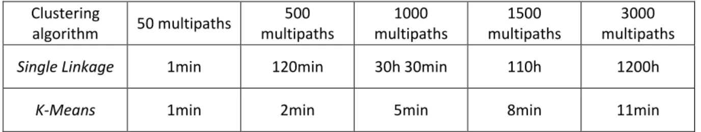
Table 2.1 : Computation time of the different clustering algorithms for different number of multipaths in the reference channel ... 87 Table 3.1: Computation time of SAGE to reduce every impulse response samples of the reference
scenario ... 117 Table 4.1 : Example of 5 realizations of the RNG process applied to the present delay distribution
conditioned by the previous delay ... 133 Table 4.2 : Example of 5 realizations of the RNG process applied to the present amplitude
distribution conditioned by the present delay and the previous amplitude ... 133 Table 4.3 : 10 realizations of the delay drawing process on the pdfs at t=5s and t=15s ... 139 Table 4.4 : 10 realizations of the amplitude drawing process on the pdfs at t=5s and t=15s ... 141 Table 5.1 : Mean (M), Standard deviation (STD), 95th and 99th percentiles (95P and 99P) of the
distributions of the discriminator error difference with the reference channel ... 158 Table 5.2 : Mean (M), Standard deviation (STD), 95th and 99th percentiles (95P and 99P) of the
distributions of the discriminator error difference with the reference channel for 3, 5, 8 and 10 MP ... 162 Table 5.3 : Configuration of the GNSS receiver GeneIQ ... 164 Table 5.4: Mean (M), Standard deviation (STD), 95th and 99th percentiles (95P and 99P) of the
distributions of the discriminator error difference with the reference channel ... 168 Table 5.5 : Mean (M), Standard deviation (STD), 95th and 99th percentiles (95P and 99P) of the
distributions of the discriminator error difference with the reference channel for 3, 5, 8 and 10 MP ... 170 Table 5.6 : Configuration of the GNSS receiver GeneIQ ... 172 Table 5.7 : Mean, standard deviation, 95th and 99th percentiles corresponding to the tracking error
difference distributions for different RF bandwidths ... 173 Table 5.8: Configuration of the GNSS receiver GeneIQ ... 173 Table 5.9 : Mean, standard deviation, 95th and 99th percentiles corresponding to the tracking error
difference distributions with noise and without noise ... 175 Table 5.10 : Mean, standard deviation, 95th and 99th percentiles corresponding to the tracking error
difference distributions with noise and without noise ... 175 Table 5.11: Mean, standard deviation, 95th and 99th percentiles corresponding to the tracking
error difference distributions considering BPSK and BOC modulated signals ... 176 Table 5.12 : Mean and standard deviations associated to distributions of discriminator error
difference for different azimuths and elevations of the emitter ... 179 Table 5.13 : 95th and 99th percentiles associated to distributions of discriminator error difference
Florian RIBAUD – PhD thesis Page 17
List of Abbreviations
3CM Three Components Model BOC Binary Offset Carrier
CDF Cumulative Density Function
CRIME Channel Reduction by Independent Markov Process CS Chip Spacing
DLL Delay Lock Loop DOA Direction of Arrival EMLP Early Minus Late Power
ESPRIT Estimation of Signal Parameters via Rotational Invariance Techniques GNSS Global Navigation Satellite System
GO Geometrical Optic
GPS Global Positioning System LHCP Left Handed Circular Polarization LMS Land Mobile Satellite
LOS Line Of Sight
ML Maximum Likelihood MOM Method of Moments
MUSIC Multiple Signal Classification NLOS Non Line of Sight
PDF Probability Density Function PLL Phase Lock Loop
PO Physical Optic
RHCP Right Handed Circular Polarization RNG Random Number Generator
SAGE Space Alternating Generalized Expectation Maximization SCHUN Simplified Channel for Urban Navigation
TDL Tap Delay Line
Florian RIBAUD – PhD thesis Page 18
Introduction
a
.
PhD thesis background and motivationsThe need of an unmasked and accurately synchronized signal to provide navigation information takes a major advantage of the large areas covered by the satellites in MEO (Medium Earth Orbit). Recently, the innovative steps in the navigation domain mainly concern the design of more complex signal models. They aim at improving the accuracy of the navigation information and improving the robustness of the system to signal perturbations, like interferences, noise or multipath for example. The GALILEO European project has been conducted in that prospect. It is supposed to be fully deployed by 2020.
Nowadays, the satellite navigation development is challenged by the increasing interest in high precision positioning in urban areas. The density of obstacles may lead to signal perturbations of the signal through the possible loss of LOS (Line Of Sight) or superposition of multipath to the useful signal. Many applications could benefit from improved urban positioning. They include LBS (Location Based
Services), ITS (Intelligent Transport Systems), augmented reality, vehicle lane control, advanced rail
signaling and navigation for the blind. Therefore, the multipath issue for GNSS receivers (in particular for future Galileo or multi-constellation receivers) is of utmost interest. The use of this kind of receivers in more and more challenging environments (for example urban areas) necessitates to deeply investigate the GNSS performances of the system in real environment, as well as assessing the adequate mitigation techniques.
The multipath phenomenon is indeed one of the most serious threats to accuracy in GNSS navigation. Multipath is the phenomenon whereby a signal arrives at a receiver with multiple paths due to reflection and diffraction of the electromagnetic waves. The multipaths take longer paths to the antenna than the direct signal, resulting in the distortion of the carrier and code of the GNSS signal. Hence a degradation of the performance in the navigation accuracy. Multipath effect is predominant in constrained environments such as urban canyons, as the user’s GNSS antenna is surrounded by many reflecting structures (walls, trees, other vehicles, etc.). Therefore, multipaths will degrade the performances related to the GNSS applications. In addition, for pedestrian or vehicular receivers, the multipath channel is mainly caused by the environment and is then totally unpredictable and hard to model. In some cases, the multipath can be due to the reflections around the platform the GNSS antenna is located on. This is the case for sensor stations. Other specific configurations may occur, where the characteristics of the direct path or the predominant multipaths vary. This is also the case for GNSS receivers located under a vegetation layer, where the direct path is attenuated by the canopy. Some of the characteristics of multipaths may also depend on the type of users (static or dynamic), as it is the case for Doppler properties. In all these cases, the multipath channel is described by the impulse response that consists in the combination of several echoes characterized by their amplitude, phase, delay, Doppler shift and direction of arrival.
Therefore, wide-band channel models have been implemented in parallel to the development of the GNSS sector. They aim at synthesizing realistic environments and put the new receivers to test. Two major channel modelling approaches have been designed, namely statistical and deterministic approaches. As many multipath configurations may be encountered, it remains difficult to draw statistical or empirical models versatile and accurate in the same time. Furthermore, the geometry of the environment can be complex (for example in urban areas or for sensor stations) which results in high computation loads if deterministic models are used. More recent hybrid models mixing statistical and physical modules showed to be a good tradeoff between practical computational effort and realistic multipath channels. In particular, the SCHUN simulator (Simplified Channel for Urban
Florian RIBAUD – PhD thesis Page 19 Navigation), developed at the ONERA by Mehdi Ait-Ighil and its PhD supervising team [AIT 12] has shown to be able to model the LOS and multipath channel through the virtual city concept. Its accuracy is close to purely physical models, with computational performance close to real-time.
However, the large number of echoes synthesized by the model (several thousand per impulse response snapshot) limits its utilization for the testing of navigation systems. Indeed, these models are used to assess the performance of GNSS receivers in multipath environment. In particular, the Galileo system is assessed to test the specificities of the signal (BOC/MBOC modulation, long and tiered codes) for multi-constellation and diversity techniques. Today, multi-frequency techniques as well as diversity antenna techniques provide the GNSS positioning with high precision in urban areas. The introduction of Galileo and the modernization of the GNSS constellation give rise to new opportunities for the development of these mitigation techniques which take advantage of multi-frequency characteristics. Nevertheless, the definition of new algorithms using several frequencies requires a good knowledge of the parameters of the channel in order to take benefit of possible information redundancies. Then, the multipath models have to be integrated either in software or hardware simulators. The testing of both software and hardware receivers suffer from large impulse responses. For software simulators, the computing time may be critical. For hardware simulators, the generation of each multipath signal requires an additional channel, then increasing the complexity and cost of the equipment. This is the reason why the models have to be simplified. The reduction techniques have to be applied to the channel model in order to limit the number of echoes without decreasing too much the representativeness of the channel in terms of receiver’s performance.
b. PhD thesis objectives
For that reason, it has been decided to focus this thesis on the analysis of solutions to decrease the number of echoes in the channel impulse responses, all by preserving the original accuracy of SCHUN to model the effect of realistic environments on the pseudo-range error of the receiver. In the scope of [AIT 13], it has been decided to implement a reduction technique making the SCHUN model adaptable to the constraints of hardware signal emulation, respecting these accuracy specifications, with practical implementation facilities (in terms of computation time essentially).
The approach chosen to address this problem can be divided in two main steps. On one side, different reduction methods will be designed and implemented. On the other side, they will be compared through the criterion of the preservation of the pseudo-range error. Three different reduced channel models have been considered. Among these models, two main approaches can be identified. Indeed, the two methods referred to as Weighted Clustering and Statistical method are dedicated to the preservation of the channel characteristics in terms of power-delay profile and/or Doppler spectrogram. They rely on the aggregation of multipaths and the statistical selection of multipaths respectively. Both methods are low demanding in terms of computational resource. The parametric optimization approach is dedicated to the conservation of the open loop discriminator error. It relies on an optimization process, heavier in terms of computational costs. The comparison of these approaches according to the pseudo-range error preservation compares the performance of low demanding methods relatively to heavier optimization processes.
c. PhD thesis outline
Chapter 1 introduces the problem of modelling the multipath channel. The first section presents different channel models extracted from the literature. They are divided in three approaches: statistical, deterministic and physical-statistical models. Then, a section has been dedicated to the
Florian RIBAUD – PhD thesis Page 20 presentation and the validation of a specific hybrid model, namely SCHUN (Simplified Channel for
Urban Navigation). This simulator will be used as the reference channel model in the following of this
thesis. Finally, the limitations to adapt these channel outputs to the testing of GNSS receivers motivates the channel reduction.
Chapter 2 focusses on the reduction of the multipath channel by aggregating multipaths. The question addressed all along this chapter is: “which parameters have to be taken into account to aggregate the echoes?”, and “which algorithm would be the most efficient in terms of preservation of the characteristics of the original channel and in terms of computation time”. As a preliminary study, a simple selection method on the multipath power has been performed. Then, in order to optimize the preservation of the delay spread, different Tap Delay Line models have been implemented. In the following sections, the Doppler shift criterion has been added to the aggregation process. Different clustering techniques have been implemented for that purpose. Finally, the method referred to as Weighted Clustering has been proposed. It aims at preserving the characteristics of the original channel with a low computational effort. It consists in aggregating the closest multipaths in terms of delay and Doppler shift, so as to improve the stability of the echoes of the reduced channel.
Chapter 3 presents the implementation of a parametric optimization process. It aims at optimizing the parameters of the reduced channel (delay, complex amplitude and Doppler shift of the multipaths) so as to conserve the channel correlation function. After introducing the cost function related to this process, the general architecture of the SAGE algorithm chosen to address this problem is presented. A particular attention is brought to the Doppler resolution of the algorithm, which has a strong impact on its performance. More specifically, the optimal tradeoff between Doppler resolution and number of echoes in the reduced channel is investigated, in order to implement an optimal parameterization method.
Chapter 4 investigates the possibility to draw multipaths of the reduced channel from their statistical distribution. It will be considered that each echo follows a first-order Markov process. A critical analysis of the method CRIME presented in [Schu 14] is performed. In particular, the technique used compute the amplitudes and delays is criticized. In that scope, an innovative semi-statistical reduction method is proposed. According to this new method, the delays of the echoed are drawn statistically, while the complex amplitude is deduced from the impulse response continuous power-delay profile.
Chapter 5 performs the comparison of the reduction methods presented in chapters 2, 3 and 4 in terms of preservation of the pseudo-range error. The comparison process is restricted to the Weighted Clustering, the parametric optimization method and the modified statistical method. First, a state-of-the-art of the different comparison frameworks of the literature is presented. To initiate the comparison, the only impact of the reduction methods on the open loop discriminator error is considered. From these results, a hierarchy among the reduction methods is established. This simulation is transposed to different positions of the emitter satellite and different numbers of echoes in the reduced channels, in order to emphasize their possible impact on this hierarchy. Then, the impact of the tracking loops of the receiver has been investigated, using the receiver simulator GeneIQ, briefly presented in this chapter 5. From that comparison, another hierarchy is established. Different signal parameters (modulation and bandwidth) have been considered to widen the scope of these results. A particular attention is brought to the impact of the elevation of the emitter satellite on this hierarchy, which turns out to have a significant impact on the performance of the reduction methods. Finally, the conclusion of this thesis decides which method is the most well suited to address the channel reduction problem, putting into balance the computational resource required by each approach.
Florian RIBAUD – PhD thesis Page 21 d. PhD thesis contributions
This thesis investigates the most efficient method to address the channel reduction problemat. All along this study, different results will be presented:
Implementation of the Clustering Weighted method, which shows a very good efficiency in terms of Doppler and delay conservation with low computational effort. The pseudo-range error caused by the original channel is also well preserved (almost as well as parametric optimization methods).
Development of a method to parametrize the reduced channel multipaths so as to preserve the channel autocorrelation function, using the SAGE algorithm. Determination of the ideal tradeoff between Doppler resolution of the algorithm and number of echoes in the reduced channel to improve the algorithm’s efficiency.
Implementation of a statistical method to draw the reduced channel multipaths from a specific stochastic process, adapting the model of [Schu 14] the constraint of larger impulse responses.
Comparison of the three aforementioned approaches according to the preservation of the pseudo-range error of the receiver. Different signal parameters and tracking configurations have been considered. The most efficient approach is identified, taking the computational load into balance.
Implementation of the discriminator open-loop error, to investigate the efficiency of the reduction methods with a validity index easy to implement. Development of a close formula to compute it from the impulse response parameters. Validation of this criterion comparing its results to those of more elaborate models of GNSS receiver.
These results have been presented at the occasion of international workshops. The following papers have been elaborated and presented:
F. Ribaud, M. Ait-Ighil, J. Lemorton, O. Julien, F. Perez-Fontan, F. Lacoste, S. Rougerie, “Comparison of different methods to aggregate multipaths for GNSS receivers performance assessment“, ENC 2015, Bordeaux, France.
F. Ribaud, M. Ait-Ighil, S. Rougerie, J. Lemorton, O. Julien, F. Pérez-Fontan, “Reduction of the Multipath Channel Impulse Response for GNSS applications”, EuCAP 2016, Davos, Switzerland.
F. Ribaud, M. Ait-Ighil, S. Rougerie, J. Lemorton, O. Julien, F. Pérez-Fontan, “Reduced multipath channel modelling preserving representative GNSS receiver testing”, ION GNSS+2016, Portland, USA.
Florian RIBAUD – PhD thesis Page 22
Chapter 1
1. Modeling of the LMS channel and introduction to the
problem of channel reduction
This chapter has been designed to introduce the channel reduction problem addressed in this thesis and to present the different concepts useful to lead this study. The first section will present the channel models of the literature, focussing on urban environments. Both statistical and deterministic approaches will be presented with a critical analyse of each method, in order to justify the use of hybrid (both statistical and physical) approaches. The second section will be devoted to the presentation of the SCHUN (Simplified CHannel for Urban Navigation) channel simulator. It has been used all along this thesis to generate the reference channels (the reduction methods will be applied on these impulse responses). Finally, the third section will illustrate the constraints caused by the large number of multipaths synthesized by SCHUN, from the point of view of a GNSS receiver. This section will introduce the necessity to implement reduction methods to reduce the reference impulse responses, which is the main work of this thesis.
Florian RIBAUD – PhD thesis Page 23
1.1. Different approaches to model the LMS channel
A significant number of urban channel models have already been proposed. They can be grouped in three major families, namely the statistical, deterministic and hybrid physical-statistical models. The presentation of these different families will constitute the three subsections of this section. The major difference between statistical and deterministic approaches relies in the trade-off between accuracy, versatility and computational load of the methods. The hybrid physical-statistical approaches try to take benefit of the advantages of both approaches, while erasing their drawbacks.
The following sub-sections will distinguish the modelling of the environment itself from the computation of the interactions between the signal and the environment. Indeed, some channel models mix statistical distribution of the environment and deterministic computation of the channel parameters and vice-versa.
1.1.1. Statistical approaches
The statistical channel approaches consist in fitting empirical models on experimental data obtained during measurement campaigns. As a first approach of the problem, it can be mentioned the narrow-band models, which aim at reproducing the time-series of signal attenuation. However, such approaches can be shortcoming to simulate the shadowing effect. Therefore, the state oriented models have been introduced in the literature. They mainly rely on the Markov chain theory. The Markov states represent the different shadowing levels of the signal. However, the only consideration of the narrow band channel characteristics is not enough in GNSS navigation contexts. The multipaths have a strong impact on the positioning performance of the receiver. The modeling of the multipath amplitude, phase, delay and Doppler shift is of utmost interest for GNSS applications. Therefore, wide-band models have been implemented.
1.1.1.1.
The narrow-band statistical modelsThe environment of the receiver has two major impacts on the channel narrow-band power: the shadowing and fast fading effects. It was already mentioned that the shadowing constitutes the signal blockage by canonical objects of the environment whereas the fast fading effect is due to the constructive or destructive combination of multipaths at the receiver antenna.
Florian RIBAUD – PhD thesis Page 24 Fig. 1.1 illustrates the impact of the fast fading and shadowing effects on the narrow-band power of the channel. The right plot represents the narrow-band power received by the GNSS receiver along its trajectory. This power is normalized by the nominal LOS power. The left plot represents the environment corresponding to this scenario. The narrow-band power has been computed by the SCHUN model, which will be detailed in section 1.2. The shadowing effect causes the power fading segments extended in time. They have been spotted by the red arrows and are due to the presence of buildings between the receiver and the incident signal. The three buildings in question are apparent on the left plot of Fig. 1.1. The fast fading effect causes the high-frequency attenuation. It has been spotted by green arrows.
The shadowing and the fast fading have distinct impacts on the time-series. Therefore, it is difficult to define a statistical distribution simulating jointly the shadowing and the fast fading. The merging models, like [Pere 01], consider the probability to be in LOS (Line Of Sight) or NLOS (Non Line of Sight) on one hand and the distribution of the fast fading effect on the other hand. This distribution depends on the LOS or NLOS condition. Among the most commonly used statistical models of the narrow-band channel, the Rayleigh and Rice distributions can be cited:
The Rayleigh distribution is used to model the fast fading in NLOS conditions. The multipaths distorting the narrow-band channel power are supposed to be statistically independent in terms of delay and phase. Eq. 1.1 displays the density function associated to the Rayleigh distribution. It depends on the fast fading standard deviation 𝜎, which is estimated from experimental data in a given environment. The variable 𝑟 is referred to as the Rayleigh variable and corresponds to the norm of a complex vector whose real and imaginary parts are Gaussian distributions of mean 0 and standard deviation 𝜎.𝑓(𝑟) = 𝑟 𝜎2𝑒−𝑟
2/2𝜎2
(1.1)
The Rice distribution is used to model the fast fading effect on one side and the LOS component on the other side. Therefore it is used to model the effects of a multipath environment considering that a certain proportion of the direct path reaches the receiver. It is characterized by the Rice factor noted 𝐾, which represents the ratio between LOS and multipath power. Several methods have been developed to estimate this parameter from experimental data [Tepe 03]. Eq. 1.2 displays the density function of the Rice distribution, considering the Rice factor K and the standard deviation 𝜎 for the fast fading. Note that 𝐼0 corresponds to the modified Bessel function of first kind and order zero.𝑓(𝑟) =2(𝐾 + 1)𝑟 𝜎2 𝑒 −𝐾−(𝐾+1)𝑟2 𝜎2 𝐼 0(2𝑟√ 𝐾(𝐾 + 1) 𝜎2 ) (1.2)
Those two distributions have been presented in this section because they are commonly used to model the narrow-band channel. However, other distributions can be used. Two examples will be cited hereafter to simulate the shadowing and fast fading effects according to a statistical approach (and eventually the design of the environment).
The Loo distribution gives the possibility to tune both LOS and multipath components, using a lognormal distribution characterized by its mean and standard deviation (𝛼, 𝜑) and a Rayleigh distribution [Pere 01] respectively.
The log-normal distribution is commonly used to characterize the environment, and more specifically the dimensions of the buildings or streets of the virtual cities. Such models allow the simulation of both LOS/NLOS and multipaths from a deterministic point of view. It will be detailed in the following sections.
Florian RIBAUD – PhD thesis Page 25 As a conclusion, those models are designed to predict the coherent and incoherent fading effects considering a given state of LOS blockage. However, they are inadequate for environments with fast fading variations. Therefore, state-oriented models have been introduced.
1.1.1.2. The state oriented statistical models
The Markov chain approach has been developed because it is well suited to model the switch from one state of shadowing to another. The probability of transition defines a Markov chain with discrete time and discrete states. It means that the probability of fading at a given instant is influenced by the fading at the predecessor instant. The number of discrete states defines the number of diverse shadowing levels of the environment. Usually 2 or 3 states are considered. Note that the slow fading effect of the complex envelope is fully characterized by the state vector 𝑃 and the transition probability matrix 𝑄 of the Markov chain.
The fast fading fluctuations are modeled by various probability distributions that are specific to each state. Therefore, the narrow-band channel is fully characterized by 𝑃, 𝑄 and the parameters of the fast fading statistics inside each state. These parameters are usually estimated from measurement campaigns. Three examples of state-oriented channel models are mentioned hereafter:
• The Lutz model has been proposed in [Lutz 91]. It considers two shadowing levels referred to as ON and OFF states. The ON state corresponds to the pure LOS condition whereas the OFF state corresponds to total signal blockage (NLOS). The Rice and Log-normal distributions are used to model the fast fading effect in LOS and NLOS states respectively.
• A 3-states Markov model has been proposed in [Pere 05]. In that case, three distinct shadowing levels are considered. State 1 corresponds to pure LOS conditions. State 3 corresponds to pure NLOS conditions. State 2 is an intermediate shadowing level between State 1 and State 3. Typically, State 3 can be linked to the signal blockage by buildings, whereas State 2 corresponds to softer attenuations, like trees for example.
The model referenced under ITU-R P681 may also be mentioned as a 2-states Markov model, with a statistical shadowing distribution inside each state [ITU 15].
Fig 1.2 illustrates a 2-states Markov chain of the first order. As it is represented on the left plot, such a model is well suited to represent the time series of Fig. 1.1. The fast fading variations can be modeled by a Rice distribution in LOS state and a Rayleigh distribution in NLOS state.
Florian RIBAUD – PhD thesis Page 26 Both fading and fast fading effects can be modeled by Markov chains. Therefore, it is an improvement to the distributions presented in sub-section 1.1.1. However, it can be noted that only the narrow-band characteristics of the channel were considered so far. In the present thesis, the channel modeling problem is dedicated to the calibration of the receiver pseudo-range error. Therefore, the wide-band parameters of the channel, such as multipath delays and Doppler shifts, have a major interest. Thus, the narrow-band channel models are shortcoming, and the wide-band models have to be investigated.
1.1.1.3. The wide-band statistical models
Most of the literature dealing with the statistical modeling of the wide-band channel relies on the WSSUS assumptions (Wide-Sense Stationarity for Uncorrelated Scatterers), which are developed in [Bell 63]. Those assumptions are fulfilled only if the channel autocorrelation remains constant and if the delay and Doppler of the Scatterers remains uncorrelated. Due to the possible non-uniform distribution of the scatterers in the azimuthal plane, those assumptions tend to restrain the field of application of such approximations. However, a few models based on the WSSUS have been developed. Some of the most worth mentioning are cited in the following. This list of models does not aim at making the reader fully familiar with these approaches, but at giving an overview of the different techniques that have been considered so far. More complete descriptions and other models can be found in [Ait 13], [Satn 08] and [COST 02].
The model of Saleh and Velenzuela [Sale 87] was designed for indoor propagation modeling. It proposes to group the multipaths of the wide band channel in clusters, according to observations made on a measurement campaign [Sale 87]. The delays of the clusters are characterized by a Poisson distribution, as well as the delays of the multipaths inside each cluster (with different 𝜆 parameters). The amplitudes of the multipaths are determined by Rayleigh distributions, whose standard deviation decreases with the delays of the multipaths.
The model introduced by Jahn [Jahn 96] relies on the same measurement campaign as [Sale 87]. The LOS component is modeled using Rice or Rayleigh distributions, depending on the shadowing level. The multipaths are divided in two delay zones, corresponding to near and far delay echoes. Among the near delay multipaths, the number of echoes is given by a Poisson law. Their delays are scaled using a Tap Delay Line technique and their amplitudes decrease according to an exponential law. Among the far echoes, their number is given by a Poison law as well but their amplitudes follow a Rayleigh distribution.
The model of Perez-Fontan introduced in [Pere 01] was already mentioned and comprises a wide-band component. From an overall point of view, it is constituted of both wide-band and state-oriented approaches. The Markov states are used to characterize the different shadowing levels of the LOS component, completed with a log-normal distribution to create low LOS fluctuations. In what concerns the multipaths channel, the principle of this model is to simulate the main contributions of the delay line, constituted by the LOS and the major rays (generated by specular reflection). These components are followed in delay by a cluster of multipaths whose delays follow an exponential distribution. The amplitude of the multipaths decreases according to linear decays whose slope depends on the Markov state.
In this non-exhaustive list of models, no generation of virtual environment was considered. It must be mentioned that this limitation is likely to lead to unrealistic multipath modeling in some cases.
Florian RIBAUD – PhD thesis Page 27 1.1.1.4. Synthesis on the statistical channel models
The presentation of the different statistical channel models allowed identifying the major advantages and drawbacks of this approach. They are discussed hereafter. Those different points motivated the development of other types of channel models.
The statistical methods give the possibility to apply simple statistical distributions to different types of scenarios, in order to simulate the narrow-band and wide-band characteristics of the LMS channel. Therefore, the main advantage of the statistical models is their ease of implementation and the low computation load. Moreover, the different statistical distributions that were described all along the previous sub-sections are easily adaptable from one scenario to another. Indeed, only few parameters have to be tuned in order to transpose it to other navigation situations.
However, it was mentioned that the parameters of those different models are extracted from experimental data. Therefore, it can be expected that various experimental data are required to fit the parameters to specific navigation situations. In order to take into account the specific features of a given environment, some data corresponding to a close environment have to be available. The more accurate the statistical channel model is, the more data are required to make it versatile. In order to consider every possible environment type, signal angle of arrival, polarization and frequency band, modulation and trajectory, very extensive measurement campaigns are required. Some other types of approaches have to be investigated in order to increase the channel accuracy.
1.1.2. Deterministic channel models
1.1.2.1. General principle
The deterministic channel approaches consist in computing the LMS channel narrow-band or wide-band parameters by modeling physically the different interactions of the impinging wave front with the environment surrounding the receiver. It requires the knowledge of the canonical elements composing the LMS channel and the characteristics of the wave, such as polarization and angle of arrival. From these data, the resulting electromagnetic wave reaching the receiver is computed. Note that such methods are possible thanks to the recent improvements of the computing tools allowing sufficient computational effort to perform such calculations.
The deterministic methods all rely on the resolution of the Maxwell's equations on the physical representation of the environment of the receiver. However, the deterministic models differ in the different assumptions and simplifications made to perform suitable computations. From that perspective, the deterministic methods can be divided in two families, namely full-wave methods and asymptotic methods.
The full-wave methods consist in solving the EM problem with no simplification assumption, which makes it adaptable to any scenario with a suitable knowledge of the physical composition of the environment (i.e. material EM properties). However, such methods are not applicable to large scenarios, because of the fast augmentation of the computational effort with the size of the environment as it will be explained in section 1.2.2.
The asymptotic methods regroup different simplifications of the original full-wave method. Such considerations generally imply some assumptions on the structure of the environment and on the position of the receiver. Nevertheless, these methods have the advantage to be applicable to a wide range of scenarios, contrary to full-wave methods. The most worth mentioning approaches will be briefly presented in section 1.2.3.
Florian RIBAUD – PhD thesis Page 28 1.1.2.2. The full-wave methods
The full-wave methods are also considered as exact methods because they do not rely on any assumption. As mentioned in the previous sub-section, the drawback of the exact methods is the computational effort required. Indeed, in order to ensure the numerical convergence to the solution of the problem, the environment has to be meshed in objects whose size is typically between λ/5 and λ/10, which increases the number of unknowns in the Maxwell equations.
The full-Wave methods regroup different techniques, which differ in the formalism considered to solve the Maxwell’s equations. One of these methods is referred to as MoM (Method of Moments). It consists in computing the EM wave reaching the receiver from the radiation of the currents induced on the physical environment by the impinging wave. This method requires to take into account boundary conditions on each considered object, leading to high computation load. Only recent improvements on matrix inversion capacities allowed sufficient computing skills to realize such calculations. Also worth mentioning as full-Wave methods are the FEFD (Finite Element in Frequency
Domain) and FDTD (Finite Difference in Time Domain). They address the Maxwell’s equations from a
differential point of view and in the temporal domain respectively.
Despite the augmentation of the computation resources, such methods require a prohibitive computation time and computer memory, increasing rapidly with the complexity of the environment. Generally, the dimensions of the scenario are limited to a magnitude of several tens of wavelengths. This thesis deals with the modeling of wide environments. Therefore these methods are remote from the field of applications of this study and do not intervene in the following chapters.
However, being given the accuracy of these methods to model the electromagnetic field and its adaptation capacities, the full-wave methods have been implemented in different applications, such as antenna radiation modeling or RCS (Radar Cross Section) computation. An example of such an implementation is the Elsem3D software in the Electromagnetic and Radar department at the ONERA, which relies on the MoM theory.
1.1.2.3. The asymptotic methods
The asymptotic methods regroup different approaches to model the electromagnetic field. They are characterized by the different simplifications and assumptions simplifying the resolution of the electromagnetic problem. Therefore, these models differ from the exact methods of the previous sub-section insofar as the Maxwell equations are not addressed rigorously but on larger surfaces (large compared to the wavelength), on which the surface currents are considered uniform. In order to satisfy this approximation, different assumptions can be made, which lead to different asymptotic solutions to the electromagnetic problem. They can be divided in two major families: optical-ray and current based methods.
The optical-ray approach relies on the modeling of electromagnetic rays according to the Fermat’s principle with different assumptions like GO (Geometrical Optics) or UTD (Universal Theory
of Diffraction) for example. The GO approach is constituted of two major ray modelling methods: the
SBR (Shooting and Bouncing Ray) and RT (Ray Tracing) methods. The SBR methodology consists in emitting EM rays in every direction around the transmitter, computing the interaction of each of these rays with the environment (reflection, diffraction or scattering) and combining the resulting rays reaching the receiver. The RT method consists in the recursive formation of the image of the signal sources by every object of the environment. A more complete presentation of these methods can be found in [COST 02]. Note that SBR and RT both require a complete knowledge of the environment of the receiver. The UTD consists in modelling the electromagnetic field resulting of the wave diffraction by edges of the environment along a single ray. The point of origin of this ray is located along the
![Figure 1.9 : Density function of the scatterers positions from the measurements of [Lehn 08]](https://thumb-eu.123doks.com/thumbv2/123doknet/3108704.88241/37.892.235.646.105.409/figure-density-function-scatterers-positions-measurements-lehn.webp)