This is an author-deposited version published in:
http://oatao.univ-toulouse.fr/
Eprints ID: 13622
To link to this article: DOI: 10.1109/LSP.2014.2369232
URL:
http://dx.doi.org/10.1109/LSP.2014.2369232
To cite this version:
Abramovich, Yuri and Besson, Olivier On the
Expected Likelihood Approach for Assessment of Regularization
Covariance Matrix. (2015) IEEE Signal Processing Letters, vol. 22 (n° 6).
pp. 777-781. ISSN 1070-9908
O
pen
A
rchive
T
oulouse
A
rchive
O
uverte (
OATAO
)
OATAO is an open access repository that collects the work of Toulouse researchers and
makes it freely available over the web where possible.
Any correspondence concerning this service should be sent to the repository
administrator:
[email protected]
On the Expected Likelihood Approach for
Assessment of Regularization Covariance Matrix
Yuri I. Abramovich, Fellow, IEEE, and Olivier Besson, Senior Member, IEEE
Abstract—Regularization, which consists in shrinkage of the
sample covariance matrix to a target matrix, is a commonly used and effective technique in low sample support covariance matrix estimation. Usually, a target matrix is chosen and optimization of the shrinkage factor is carried out, based on some relevant metric. In this letter, we rather address the choice of the target matrix. More precisely, we aim at evaluating, from observation of the data matrix, whether a given target matrix is a good regularizer. Towards this end, the expected likelihood (EL) approach is inves-tigated. At a Þrst step, we re-interpret the regularized covariance matrix estimate as the minimum mean-square error estimate in a Bayesian model where the target matrix serves as a prior. The likelihood function of the data is then derived, and the EL prin-ciple is subsequently applied. Over-sampled and under-sampled scenarios are considered.
Index Terms—Covariance matrix estimation, expected
likeli-hood, regularization.
I. PROBLEMSTATEMENT ANDMOTIVATION
E
STIMATION of the covariance matrixof a random vector from a Þnite number
of independent observations is a
fun-damental problem in many engineering applications. For in-stance, in adaptive radar detection where it is desired to detect a target buried in Gaussian noise, the optimal Þlter depends on the noise covariance matrix, and the latter is usually estimated from training samples which contains noise only noise only [1], [2]. However, substituting the sample covariance matrix (SCM) for in the optimalÞlter results in a signiÞcant loss in terms of output signal to noise ratio (SNR) [3], [4]. Indeed, the corresponding SNR loss is beta distributed and approximately samples are required to achieve an average SNR loss less than 3 dB. In cases where is large, this number can be prohibitive and it is more customary to have to operate in low sample support. To cope with such situations, a widely used technique consists in regularization, or shrinkage of the SCM
;
Y. Abramovich is with WR Systems, Ltd., Fairfax, VA 22030 USA (e-mail: [email protected]).
O. Besson is with the University of Toulouse, ISAE-Supaero, Department Electronics Optronics Signal, Toulouse, France (e-mail: [email protected]).
towards a given matrix , i.e., estimate as, see e.g., [5], [6], [7], [8]
(1) where and is some matrix, which is deemed to be close to [6] or is meant at regularizing the problem. The par-ticular case of (often referred to as diagonal loading) has proven to be particularly effective, especially when the noise has a high-power low-rank component plus a white noise com-ponent [9], [10], [11]. However, other possible choices are pos-sible, including colored loading [12], [13]. Most often, is Þxed and its choice is not questioned: rather, the focus is on op-timization of , so as, for instance, to achieve minimum mean-square error of the estimate in (1). Even if is adequately se-lected, the choice of may also be very inßuential. For instance, diagonal loading is known to perform better when the eigen-spectrum of the covariance matrix consists of a few dominant eigenvalues plus a Þxed ßoor: it may not be as effective when the eigenspectrum has a smoothly decreasing proÞle.
In this paper, we address the selection of . More speciÞcally, we wish to examine whether is a good choice as a regularizer, from observation of . Towards this end, we propose to use the expected likelihood (EL) approach [14], [15], [16] to assess the plausibility of . The EL was introduced as a tool to assess the quality of a covariance matrix estimate, say for example . It relies on some invariance properties of the likelihood ratio (LR) for testing if . In [14], [15], [16], it was proved that the LR, evaluated at the true covariance matrix of , has a distribution that only depends on and . This property led the authors of [14], [15], [16] to select such that the value of is commensurate with that taken at the true covariance matrix. In this paper, we investigate using the EL approach not for selection of , rather for that of .
II. ASSESSMENT OF THROUGHEXPECTEDLIKELIHOOD
In this section, we use the EL approach to evaluate the plausibility of the regularization covariance matrix . First, the estimate in (1) is re-interpreted as the minimum mean-square error (MMSE) estimate of in a Bayesian framework where
serves as a prior covariance. Then, the likelihood
corresponding to this model is derived and shown to be of a multivariate Student distribution type. Finally, the EL approach is applied to this Student distribution. Let us assume that the columns of are independent and identically distributed random vectors drawn from a zero-mean complex multivariate
Gaussian distribution, which we denote as . Then, the probability density function (p.d.f.) of is given by
(2) where stands for the exponential of the trace. Suppose now that is drawn from an inverse Wishart distribution with
degrees of freedom and mean , i.e., its p.d.f. is given by
(3) where means proportional to. We denote this distribution as . Then, the posterior distribution
of is
(4)
with . Therefore,
and the MMSE of
is the mean of (4), i.e., [17]
(5) which is exactly of the form (1). It follows that the regularizing matrix in (1) is equivalent to a prior covariance matrix in the Bayesian model (2)-(3). Choosing thus amounts to choosing a prior covariance matrix.
Next, this interpretation paves the way to using the EL ap-proach. At Þrst glance, it is not obvious why and how the EL approach could be used in the purpose of testing the plausibility of in the Bayesian hierarchical model described by (2)-(3), as the latter is quite different from the framework the EL approach was originally based upon. However, one should observe that , and hence is the “average” covariance matrix of . Additionally, the p.d.f. of can be written as [18]
(6) which is recognized as a multivariate Student distribution with
degrees of freedom and parameter matrix
[19], [20]. Before pursuing our derivations, we would like to offer the following comments. Let denote a square-root of , i.e., . In the Bayesian model (2)–(3), one has [18],
[19] where means “is distributed
as”. In the previous equation, follows a Wishart distri-bution with degrees of freedom and parameter matrix ,
i.e., . We denote the
Wishart distribution as . It ensues that (7)
with independent of . In
con-trast, (6) yields the representation [19], [20]
(8)
where . Albeit the two
mechanisms for generating are different, from a likelihood point of view the two representations are equivalent, as far as only assessment of from is involved. Of course, in the Bayesian model (2)-(3), serves as a prior, and interest is on estimating , while in (6), is viewed as the covariance matrix in a Student distribution. Nevertheless, from our perspective of evaluating the plausibility of , we will be using (6) and there-fore the EL approach can be advocated. Observe that the differ-ence compared to the original Gaussian frequentist framework of [14], [15], [16], is that one needs to deal with a Bayesian hier-archical framework which results in a non Gaussian likelihood . This being so, the EL approach was recently extended to the class of elliptically contoured distributions (ECD) [21], [22], [23] in [24], [25], [26]. Herein, we build upon the results of [26] with a few differences due to the fact that is the av-erage covariance in a Bayesian framework. We Þrst investigate the over-sampled case ( ), then the under-sampled case ( ) which deserves a speciÞc treatment.
A. Over-Sampled Case
When , the (generalized) likelihood ratio for a candi-date is given by
(9)
where is the MLE of , given by [21]
(10)
Therefore, the LR for the candidate can be rewritten as
(11)
where . Let us now
evaluate this LR at the true matrix . From (7)-(8), it ensues that
(12a)
where . Hence, the likelihood ratio, when evaluated at the true matrix (i.e., when
and has
a distribution that only depends on , and . This p.d.f. can thus be computed in advance and the LR for a candidate regularization matrix , as given by (11), can be compared to, say, the median value of , to decide if is a “good” regularization matrix.
B. Under-Sampled Case
When the number of observations is less than the size of the observation space, the above theory does no longer hold since, with probability one, the data matrix belongs to a sub-space of dimension . More precisely, if we let
be the thin singular value decomposition of , inference about the covariance matrix of can be made only in the subspace spanned by the columns of [27]: in other words, only is identiÞable. As argued in [27] for Gaussian settings, if one wants to assess as the covariance matrix of , at best one can test the “closest” matrix to in . The
latter is given by with ,
and can be interpreted as a singular covariance matrix [27]. Therefore, the under-sampled scenario is closely related to dis-tributions with singular covariance matrices: this is indeed the starting point of the EL approach when , see e.g., [27], [25] for details.
Thus, let us start with the Student distribution (8) in the case
where has rank , i.e., where
and is an arbitrary full-rank positive deÞnite Hermitian ma-trix. We assume temporarily that is known (it will be re-placed by when coming back to our original problem). Also, let be an orthonormal basis for the complement of , i.e., and . Then, one can deÞne a singular density on the set
as [28], [29]
(13)
The MLE of is given by, see (10),
. It follows
that the likelihood ratio, for the candidate is given by (14) with
. (See (14)–(15), shown at the bottom of the page.)
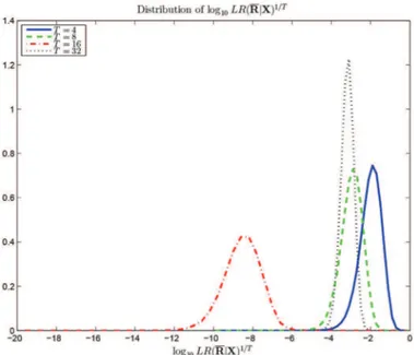
Fig. 1. Probability density function of for various . and .
Let us now come back to assessing a candidate matrix : as argued before, one can only assess the closest
ma-trix to in , namely with
. The MLE of is now given
by .
From (14), the likelihood ratio is thus given by (15) where we used the fact that . When evaluated at the true
, the stochastic representations in (7)-(8) yield
(16a)
(16b)
III. NUMERICALILLUSTRATIONS
We now illustrate how the above procedure can be helpful in assessing the validity of a given prior (or regularization) ma-trix . We consider a uniform linear array with el-ements spaced a half wavelength apart. The data are generated according to the Bayesian model (2)–(3). In Fig. 1 we display the distribution of the log likelihood ratio for different values of
(14)
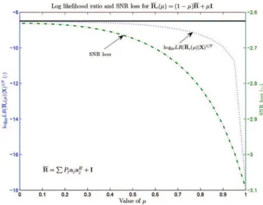
Fig. 2. Likelihood ratio of and SNR loss of asso-ciated Þlter versus . , and
. .
. Similarly to what was observed in [16], [25], the log likeli-hood ratio, when evaluated at the true takes very small values, and hence a candidate should be retained if its corresponding LR matches that of the true . Let us now investigate if this procedure results in a “good” choice for . We consider three types of covariance matrix :
1) with and . 2) with . 3) with , , , and dB
For each type, we consider as a candidate
with and we evaluate the mean value of . Note that, a priori, the best choice is . In order to assess , we consider the
adaptive Þlter where
is the signature of the signal of interest. The SNR loss, eval-uated at the output of this adaptive Þlter, will serve as a Þgure of merit for assessment of . In Fig. 2–4, we
display the mean value of (the solid
line represents the target value, namely the median value of ), as well as the SNR loss. These Þgures conÞrm two facts. Firstly, there is a good consistency between and the fact that the Þlter based on is effective. In other words, selecting from the EL principle helps Þnding a good regular-ization matrix and, subsequently, a performant adaptive Þlter. Secondly, diagonal loading is seen to be more effective in the case of a low-rank plus white noise type of covariance ma-trix: indeed, the LR remains close to for a large range of values of , and so is for the SNR loss. In fact, choosing the identity matrix as a regularizer is as good as selecting the true . In contrast, diagonal loading is less ef-fective for the two other types of covariance matrix: when
Fig. 3. Likelihood ratio of and SNR loss of asso-ciated Þlter versus . , and
. exp .
Fig. 4. Likelihood ratio of and SNR loss of asso-ciated Þlter versus . , and
. .
increases, the LR departs from its target value and SNR loss is worst.
IV. CONCLUSIONS
In this letter, we addressed the problem of selecting the reg-ularization matrix in estimation schemes which consist of shrinkage of the sample covariance matrix to a given regular-ization matrix. We interpreted the latter as a prior covariance matrix in a Bayesian model. The likelihood function of the latter was derived as a function of , and the expected likeli-hood approach was advocated to assess the validity of . It was shown that this approach is instrumental in providing a reliable measure of the quality of . As a by-product, we showed that diagonal loading is effective only in special cases of covariance matrices, and the EL approach proposed was helpful in identi-fying these cases.
REFERENCES
[1] E. J. Kelly, “An adaptive detection algorithm,” IEEE Trans. Aerosp.
Electron. Syst., vol. 22, no. 1, pp. 115–127, Mar. 1986.
[2] F. C. Robey, D. R. Fuhrmann, E. J. Kelly, and R. Nitzberg, “A CFAR adaptive matched Þlter detector,” IEEE Trans. Aerosp. Electron. Syst., vol. 28, no. 1, pp. 208–216, Jan. 1992.
[3] I. S. Reed, J. D. Mallett, and L. E. Brennan, “Rapid convergence rate in adaptive arrays,” IEEE Trans. Aerosp. Electron. Syst., vol. 10, no. 6, pp. 853–863, Nov. 1974.
[4] C. G. Khatri and C. R. Rao, “Effects of estimated noise covariance ma-trix in optimal signal detection,” IEEE Trans. Acoust., Speech, Signal
Process., vol. ASSP-35, no. 5, pp. 671–679, May 1987.
[5] O. Ledoit and M. Wolf, “A well-conditioned estimator for large-di-mensional covariance matrices,” J. Multivar. Anal., vol. 88, no. 2, pp. 365–411, Feb. 2004.
[6] P. Stoica, J. Li, X. Zhu, and J. R. Guerci, “On using a priori knowledge in space-time adaptive processing,” IEEE Trans. Signal Process., vol. 56, no. 6, pp. 2598–2602, Jun. 2008.
[7] Y. Chen, A. Wiesel, and A. O. Hero, “Robust shrinkage estimation of high-dimensional covariance matrices,” IEEE Trans. Signal Process., vol. 59, no. 9, pp. 4097–4107, Sep. 2011.
[8] E. Ollila and D. Tyler, “Regularized M-estimators of scatter matrix,”
IEEE Trans. Signal Process., vol. 62, no. 22, pp. 6059–6070, Nov.
2014.
[9] Y. I. Abramovich, “Controlled method for adaptive optimization of Þl-ters using the criterion of maximum SNR,” Radio Eng. Electron. Phys., vol. 26, pp. 87–95, Mar. 1981.
[10] Y. I. Abramovich and A. I. Nevrev, “An analysis of effectiveness of adaptive maximization of the signal to noise ratio which utilizes the inversion of the estimated covariance matrix,” Radio Eng. Electron.
Phys., vol. 26, pp. 67–74, Dec. 1981.
[11] O. P. Cheremisin, “EfÞciency of adaptive algorithms with regularised sample covariance matrix,” Radio Eng. Electron. Phys., vol. 27, no. 10, pp. 69–77, 1982.
[12] J. D. Hiemstra, “Colored diagonal loading,” in Conf. Proc. IEEE
Radar, 2002, pp. 386–390.
[13] P. Wang, Z. Sahinoglu, M.-P. Pun, H. Li, and B. Himed, “Knowl-edge-aided adaptive coherence estimator in stochastic partially homo-geneous environments,” IEEE Signal Process. Lett., vol. 18, no. 3, pp. 193–196, Mar. 2011.
[14] Y. Abramovich, N. Spencer, and A. Gorokhov, “Bounds on maximum likelihood ratio-Part I: Application to antenna array detection-estima-tion with perfect wavefront coherence,” IEEE Trans. Signal Process., vol. 52, no. 6, pp. 1524–1536, Jun. 2004.
[15] Y. I. Abramovich, N. K. Spencer, and A. Y. Gorokhov, “GLRT-based threshold detection-estimation performance improvement and applica-tion to uniform circular antenna arrays,” IEEE Trans. Signal Process., vol. 55, no. 1, pp. 20–31, Jan. 2007.
[16] “ModiÞed GLRT and AMF framework for adaptive detectors,” IEEE
Trans. Aerosp. Electron. Syst., vol. 43, no. 3, pp. 1017–1051, Jul. 2007.
[17] J. A. Tague and C. I. Caldwell, “Expectations of useful complex Wishart forms,” Multidimen. Syst. Signal Process., vol. 5, pp. 263–279, 1994.
[18] R. J. Muirhead, Aspects of Multivariate Statistical Theory.. New York, NY, USA: Wiley, 1982.
[19] A. K. Gupta and D. K. Nagar, Matrix Variate Distributions. Boca Raton, FL, USA: Chapman & Hall/CRC, 2000.
[20] S. Kotz and S. Nadarajah, Multivariate t Distributions and their
appli-cations. Cambridge, U.K.: Cambridge Univ. Press, 2004. [21] K. T. Fang and Y. T. Zhang, Generalized Multivariate Analysis.
Berlin, Germany: Springer Verlag, 1990.
[22] T. W. Anderson and K.-T. Fang, Theory and applications of elliptically contoured and related distributions U.S. Army Research OfÞce, Tech. Rep. 24, Sep. 1990.
[23] E. Ollila, D. Tyler, V. Koivunen, and H. Poor, “Complex elliptically symmetric distributions: Survey, new results and applications,” IEEE
Trans. Signal Process., vol. 60, no. 11, pp. 5597–5625, Nov. 2012.
[24] Y. I. Abramovich and O. Besson, “Regularized covariance matrix estimation in complex elliptically symmetric distributions using the expected likelihood approach—Part I: The oversampled case,” IEEE
Trans. Signal Process., vol. 61, no. 23, pp. 5807–5818, Dec. 2013.
[25] O. Besson and Y. I. Abramovich, “Regularized covariance matrix estimation in complex elliptically symmetric distributions using the expected likelihood approach - Part 2: The under-sampled case,” IEEE
Trans. Signal Process., vol. 61, no. 23, pp. 5819–5829, Dec. 2013.
[26] O. Besson and Y. Abramovich, “Invariance properties of the likelihood ratio for covariance matrix estimation in some complex elliptically con-toured distributions,” J. Multivar. Anal., vol. 124, pp. 237–246, Feb. 2014.
[27] Y. I. Abramovich and B. A. Johnson, “GLRT-based detection-esti-mation for undersampled training conditions,” IEEE Trans. Signal
Process., vol. 56, no. 8, pp. 3600–3612, Aug. 2008.
[28] M. S. Srivastava and C. G. Khatri, An Introduction to Multivariate
Sta-tistics. New York, NY, USA: Elsevier/North Holland, 1979. [29] M. Siotani, T. Hayakawa, and Y. Fujikoto, Modern Multivariate