On Iterative Solution of the Extended Normal Equations

(1)

an author's https://oatao.univ-toulouse.fr/26815

https://doi.org/10.1137/19M1288644

Calandra, Henri and Gratton, Serge and Riccietti, Elisa and Vasseur, Xavier On Iterative Solution of the Extended Normal Equations. (2020) SIAM Journal on Matrix Analysis and Applications, 41 (4). 1571-1589. ISSN 0895-4798

(2)

ON ITERATIVE SOLUTION OF THE EXTENDED NORMAL EQUATIONS\ast

HENRI CALANDRA\dagger , SERGE GRATTON\ddagger , ELISA RICCIETTI\ddagger , AND XAVIER VASSEUR\S

Abstract. Given a full-rank matrix A \in \BbbR m\times n _{(m \geq n), we consider a special class of linear}

systems AT_{Ax = A}T_{b + c with x, c \in \BbbR}n _{and b \in \BbbR}m_{, which we refer to as the extended normal}

equations. The occurrence of c gives rise to a problem with a different conditioning from the standard normal equations and prevents direct application of standard methods for least squares. Hence, we seek more insights on theoretical and practical aspects of the solution of such problems. We propose an explicit formula for the structured condition number, which allows us to compute a more accurate estimate of the forward error than the standard one used for generic linear systems, which does not take into account the structure of the perturbations. The relevance of our estimate is shown on a set of synthetic test problems. Then, we propose a new iterative solution method that, as in the case of normal equations, takes advantage of the structure of the system to avoid unstable computations such

as forming AT_{A explicitly. Numerical experiments highlight the increased robustness and accuracy of}

the proposed method compared to standard iterative methods. It is also found that the new method can compare to standard direct methods in terms of solution accuracy.

Key words. linear systems, conjugate gradient method, forward error, least squares problems AMS subject classifications. 15A06, 65F10, 65F35, 65G50

DOI. 10.1137/19M1288644

1. Introduction. Given A \in \BbbR m\times n

, m \geq n, with rank(A) = n, b \in \BbbR m_{, and} x, c \in \BbbR n_{, we consider the extended least squares problem}

(ELS) min

x\in \BbbR n 1

2\| Ax - b\|

2_{- c}T_x,

whose solution satisfies the extended normal equations

(ENE) ATAx = ATb + c

or, equivalently, what is often known as the augmented system

(1.1) \biggl[ \xi Im A AT 0 \biggr] \biggl[ y x \biggr] = \biggl[ b - c/\xi \biggr] , r = \xi y = b - Ax,

where \xi is a scaling parameter that can be chosen to minimize the condition number of the augmented matrix. The optimal value of the scaling parameter is \xi \ast = _\surd1

2\sigma min(A) [3]. The vectors x and r are uniquely determined and independent of \xi . Equation \ast _{Received by the editors September 20, 2019; accepted for publication (in revised form) by}

M. T\r uma July 16, 2020; published electronically October 8, 2020.

https://doi.org/10.1137/19M1288644

Funding: The work of the authors was partially supported by the 3IA Artificial and Natu-ral Intelligence Toulouse Institute, French ``Investing for the Future - PIA3"" program under grant ANR-19-PI3A-0004 and by the TOTAL R\&D under grant DS3416.

\dagger _{TOTAL, Centre Scientifique et Technique Jean F\'}_{eger, F-64000 Pau, France (Henri.Calandra@}

total.com).

\ddagger _{INPT-IRIT, University of Toulouse and ENSEEIHT, F-31071 Toulouse Cedex 7, France (serge.}

gratton@enseeiht.fr, elisa.riccietti@enseeiht.fr).

\S _{ISAE-SUPAERO, University of Toulouse, F-31055 Toulouse Cedex 4, France (xavier.vasseur@}

(3)

(1.1) also gives the first-order optimality conditions for the problems (ELS-primal) min x,r 1 2\| r\| 2_{- c}T_x _{subject to} _{Ax + r = b} and (ELS-dual) min r 1 2\| r\| 2_{- b}T_r _{subject to} _AT_{r = - c.}

Using the QR factorization [A b] = Q\bigl[ R d1

0 d2\bigr] with R \in \BbbR

n\times n_{, we could obtain the} solution from

x = A\dagger b + A\dagger (A\dagger )Tc = R - 1d1+ (RTR) - 1c.

At first sight (ENE) evokes a least squares problem in the normal equations form ATAx = ATb,

but the vector c makes the situation fundamentally different. Unlike pure least squares problems, a very well-studied topic [4], [19, Chapter 5], [25, Chapter 10], problem (ENE) has not been the object of much study in the literature. We mention Bj\"orck [3], who studies the numerical solution of the augmented system by Gaussian elimination. The solution of problem (ENE) is required in various applications in optimization, such as the multilevel Levenberg--Marquardt methods [8], or certain formulations based on penalty function approaches [13], [14, section 7.2], [15], which we describe in section 2. Motivated by these important applications, we seek more insight on theoretical and practical aspects of the numerical solution of (ENE). Having in mind the possibility of seeking an approximate solution, we especially focus on iterative methods. We expect to encounter issues similar to those reported in the literature on normal equations.

First, it is well known that the product AT_{A should not be explicitly formed,} because the accuracy attainable by methods for the solution of the normal equations may be much lower than for a backward stable method for least squares. If the matrix is formed, the best forward error bound for the normal equations can be obtained by the classical sensitivity analysis of linear systems. It is of order \kappa 2(A) \epsilon with \epsilon the machine precision and \kappa (A) = \| A\| \| A\dagger \| the condition number of A in the Euclidean norm [23, 28]. This is an underwhelming result, as from Wedin's theorem [23, Theorem 20.1] the sensitivity of a least squares problem is measured by \kappa 2_{(A) only when the} residual is large, and by \kappa (A) otherwise.

However, practical solution methods do not form the product AT_{A, and the} follow-ing key observation is rather exploited. The special structure of the normal equations allows us to write

ATAx - ATb = AT(Ax - b),

which makes it possible to either employ a factorization of A rather than of AT_{A (in} the case of direct methods) or to perform matrix-vector multiplications of the form Ax and AT_{y rather than A}T_{Ax (in the case of iterative methods). The standard} analysis of linear systems is unsuitable for predicting the error for such methods, as it is based on the assumption that the linear system is subject to normwise perturbations on AT_{A. If the product is not formed explicitly, such global perturbations are not} generated in finite precision and a condition number useful for predicting the error should rather take into account structured perturbations, such as perturbations in

(4)

the matrix A only. A structured analysis is then more relevant and indeed leads to the same conclusions as for least squares problems [20].

It is therefore possible to devise stable implementations of methods for normal equations. In [22, section 10], Hestenes and Stiefel propose a specialized implementa-tion of the conjugate gradient (CG) method for the normal equaimplementa-tions, now known as CGLS. This has been deeply investigated in the literature [5, 19, 22, 27] and CGLS was shown to be more stable than CG applied directly to the standard normal equa-tion with c = 0. However, not all the consideraequa-tions made for normal equaequa-tions apply to (ENE). The presence of c has important theoretical and practical consequences.

On one hand, c results in a different mapping for the condition number and a different set of admissible perturbations for the backward error. Consequently, the existing perturbation theory for least squares problems [1, 20, 29] does not apply. A proper analysis of the structured condition number of the problem should be devel-oped.

From a practical perspective, even though the system matrix is the same, the presence of c in the right-hand side prevents direct application of standard methods for the normal equations. Successful algorithmic procedures used for normal equations can, however, be tailored to obtain stable solution methods.

Contributions. We propose CGLSc, a modification of standard CGLS that re-sults in a stable method for the solution of (ENE). We provide an expression of the structured condition number for (ENE), which allows us to compute first-order es-timates of the forward error in the computed solution. We report on the numerical performance of the method on a relevant set of test problems. The experimentation confirms improved stability of the proposed method compared to standard iterative methods such as CG and MINRES [26], and it is shown to provide solutions almost as accurate as those obtained by stable direct methods. The estimate of the forward error is also validated numerically and shown to be a sharper upper bound than the standard bound from the theory of linear systems.

Structure. In section 2 we present two applications arising in optimization where the solution of (ENE) is required. In section 3, we report on the conditioning of the problem and backward error analysis. These results are employed to propose a first-order estimate of the forward error in the solution computed by a method that does not form matrix AT_{A. In section 4 we introduce a new stable iterative method for} the solution of (ENE). Extensive numerical experiments are described in section 5. Conclusions are drawn in section 6.

, c \in \BbbR n_{, and \alpha , \beta , \gamma > 0, we define the following parameterized} Frobe-nius norm

\biggl[ \alpha A \beta b \gamma cT ₀ \biggr] \bigm\| \bigm\| \bigm\| \bigm\| F = \sqrt{} \alpha 2_{\| A\|}2 F + \beta 2\| b\| 2+ \gamma 2\| c\| 2.

We denote by In \in \BbbR n\times n_{the identity matrix of order n, by \otimes the Kronecker product} of two matrices, and by vec the operator that stacks the columns of a matrix into a vector of appropriate dimension [20].

(5)

2. Two motivating applications. We describe two different applications in which problems of the form (ELS) arise, motivating our interest in their solution.

2.1. Fletcher's exact penalty function approach. The first applicative con-text arises in equality constrained minimization. Consider a problem of the form

min

x f (x) s.t. g(x) = 0

for twice differentiable functions f : \BbbR n _{\rightarrow \BbbR and g : \BbbR}n _{\rightarrow \BbbR}m_{. The solution of} systems of the form (ENE) is needed to evaluate the following penalty function and its gradient [15], [14, section 7.2]:

\Phi \lambda (x) = f (x) - g(x)Ty\lambda (x),

where y\lambda _{(x) \in \BbbR}m_{is defined as the solution of the minimization problem} min

y \| A(x)

T_{y - \nabla f (x)\|}2_{+ \lambda g(x)}T_y

with A(x) the Jacobian matrix of g(x) at x, and \lambda > 0 a given real-valued penalty parameter.

2.2. Multilevel Levenberg--Marquardt method. The solution of (ENE) is required in multilevel Levenberg--Marquardt methods, which are specific members of the family of multilevel optimization methods recently introduced in Calandra et al. [8] and further analysed in Calandra et al. [7]. The multilevel Levenberg--Marquardt method is intended to solve nonlinear least squares problems of the form

min x f (x) =

1 2\| F (x)\|

2

with F : \BbbR n _{\rightarrow \BbbR}m _{a twice continuously differentiable function. In the two-level} setting, the multilevel method allows two different models to compute the step at each iteration: the classical Taylor model or a cheaper model mH

k, built from a given approximation fH_(xH_{) =}1

2\| F

H_(xH_)\|2 _{to the objective function}

mH_k(xH_k, sH) = 1 2\| J H_(xH k)s H_{+ F}H_(xH k )\| 2₊\lambda k 2 \| s H_\|2_{+ (R\nabla f (xk) - \nabla f}H_(xH 0)) T_sH with JH_(xH

k) the Jacobian matrix of F

H _{at x}H

k , \lambda k > 0 a real-valued regularization parameter, R a full-rank linear restriction operator, and xH

0 = Rxk with xk denoting the current iterate at a fine level.

While minimizing the Taylor model amounts to solving a formulation based on the normal equations, minimizing mH

k requires the solution of a problem of the form (ELS) because of the correction term (R\nabla f (xk) - \nabla fH_(xH

0))TsH needed to ensure coherence between levels. Approximate minimization of the model is sufficient to guarantee convergence of the method. Thus if the coarse problem is not small, an iterative method is well suited for minimizing the model.

3. Conditioning of the problem and backward error analysis. We first propose an explicit formula for the structured condition number of problem (ENE). This is useful to compute a first-order estimate of the forward error for methods that do not form matrix AT_{A explicitly. Contrary to the classical sensitivity analysis of} linear systems, which is based on the assumption that the linear system is subject to normwise perturbations on the matrix AT_{A, our result indeed considers perturbations} on matrix A only. We also propose theoretical results related to the backward error.

(6)

3.1. Conditioning of the problem. The conditioning of problem (ENE) is the sensitivity of the solution x to perturbations in the data A, b, c. We give an explicit formula for the structured condition number for perturbations on all of A, b, and c. In the following, we define the condition number of a function; see [28].

Definition 3.1. Let \scrX and \scrY be normed vector spaces. If F is a continuously differentiable function

F : \scrX \rightarrow \scrY , x \mapsto - \rightarrow F (x),

the absolute condition number of F at x is the scalar \| F\prime (x)\| := sup_{\| v\|}_\scrX=1\| F\prime (x)v\| \scrY , where F\prime (x) is the Fr\'echet derivative of F at x. The relative condition number of F at x is

\| F\prime _{(x)\| \| x\|} \scrX \| F (x)\| \scrY .

We consider F as the function that maps A, b, c to the solution x of (ENE), F : \BbbR m\times n\times \BbbR m

\times \BbbR n \rightarrow \BbbR n_, (A, b, c) \mapsto - \rightarrow F (A, b, c) = A\dagger b + A\dagger (A\dagger )Tc.

The Fr\'echet derivative in finite-dimensional spaces is the usual derivative. In par-ticular, it is represented in coordinates by the Jacobian matrix. If F is Fr\'echet differentiable at a point (A, b, c), then its derivative is

F\prime _{(A, b, c) : \BbbR}m\times n\times \BbbR m \times \BbbR n

\rightarrow \BbbR n_, F\prime (A, b, c)(E,f, g) = JF(A, b, c)(E, f, g),

where JF(A, b, c)(E, f, g) denotes the Jacobian matrix of F at (A, b, c) applied to (E, f, g). As in [20], we choose the Euclidean norm for the solution and the pa-rameterized Frobenius norm for the data (as introduced in section 1). According to Definition 3.1 (cf. also [18]), the absolute condition number of F at the point (A, b, c) is given by

\| F\prime (A, b, c)\| = sup \| (E,f,g)\| F (\alpha ,\beta ,\gamma )=1

\| F\prime (A, b, c)(E, f, g)\| , _{E \in \BbbR}m\times n_{, f \in \BbbR}m_{, g \in \BbbR}n. The parameterized Frobenius norm has been chosen for its flexibility. For instance, taking large values of \gamma allows us to perturb A and b only, and to include the case c = 0. This is because the condition \gamma \rightarrow \infty implies g \rightarrow 0 from the constraint \alpha 2_{\| E\|}2

F+ \beta 2\| f \| 2+ \gamma 2\| g\| 2= 1 in the definition of the condition number.

Let A be perturbed to \~A = A + E, the vector b to \~b = b + f , and vector c to \~

c = c + g. ATA is then perturbed to

(3.1) A\~TA = (A + E)\~ T(A + E) = ATA + ATE + ETA,

neglecting the second-order terms. The solution x = (ATA) - 1(ATb + c) is then per-turbed to \~x = x + \delta x = ( \~AT_A)_\~ - 1_{( \~}_AT\~_{b + \~}_{c). Then, \~}_{x solves}

(ATA + ATE + ETA)\~x = (ATb + ETb + ATf + c + g).

Recalling that for A of full column rank, A\dagger = (AT_A) - 1_AT _{and (A}T_A) - 1 _{= A}\dagger _(A\dagger ₎T_, we have \delta x = (AT_A) - 1_ET_{r - A}\dagger _{Ex + A}\dagger _{f + A}\dagger _(A\dagger ₎T_{g. We conclude that}

F\prime (A, b, c)(E, f, g) = (ATA) - 1ETr - A\dagger Ex + A\dagger f + A\dagger (A\dagger )Tg for all E \in \BbbR m\times n

, f \in \BbbR m

, g \in \BbbR n_{, and r = b - Ax. We then deduce the following} property.

(7)

Lemma 3.2. The conditioning of problem (ENE) with Euclidean norm on the solution and Frobenius norm (parameterized by \alpha , \beta , \gamma ) on the data, is given by (3.2) \| F\prime (A, b, c)\| = \| [((rT\otimes (ATA) - 1)LT - xT \otimes A\dagger )/\alpha , A\dagger /\beta , (ATA) - 1/\gamma ]\| , where LT is a permutation matrix consisting of ones in positions (n(k - 1) + l, m(l - 1) + k) with l = 1, . . . , n and k = 1, . . . , m and of zeros elsewhere [16, 20].

The following theorem gives an explicit and computable formula for the structured condition number.

Theorem 3.3. The absolute condition number of problem (ENE) with Euclidean norm on the solution and Frobenius norm (parameterized by \alpha , \beta , \gamma ) on the data, is \sqrt{}

\| \=M \| with \=_{M \in \BbbR}n\times n _{given by} (3.3) M =\= \biggl( 1 \gamma 2+ \| r\| 2 \alpha 2 \biggr) (ATA) - 2+\biggl( 1 \beta 2+ \| x\| 2 \alpha 2 \biggr) (ATA) - 1 - 2 \alpha 2 sym(B) with B = A\dagger rxT_(AT_A) - 1_{, sym(B) =} 1

2(B + B

T_{), and x the exact solution of (ENE).} Proof. Let us define M = [((rT_{\otimes (A}T_A) - 1_)LT_{- x}T _{\otimes A}\dagger _{)/\alpha , A}\dagger _{/\beta , (A}T_A) - 1_{/\gamma ].} We recall that

(3.4) \| F\prime (A, b, c)\| = \| M \| = \| MT\| := sup y\not =0

\| MT_y\| \| y\| . Let us consider

yTF\prime (A, b, c)(E, f, g) = yT(ATA) - 1ETr - yTA\dagger Ex + yTA\dagger f + yTA\dagger (A\dagger )Tg = rTE(ATA) - 1y - yTA\dagger Ex + yTA\dagger f + yTA\dagger (A\dagger )Tg. We recall that E =\sum n_i=1\sum m_j=1eT

i Eejfor ei, ej, the ith and jth vectors of the canon-ical basis. Then, we can rewrite the expression as

[vec(S)/\alpha , yTA\dagger /\beta , yTA\dagger (A\dagger )T/\gamma ] \cdot [\alpha vec(E), \beta f, \gamma g]T := wT[\alpha vec(E), \beta f, \gamma g]T, introducing the matrix S such that

Si,j = rTeieT_j(ATA) - 1y - yTA\dagger eieT_jx.

It follows that w = MT_{y. We are then interested in the norm of w. We can compute} the squared norm of vec(S) as

\| vec(S)\| 2= n \sum i=1 m \sum j=1 (rTeieTj(A T A) - 1y - yTA\dagger eieTjx) 2

= \| r\| 2\| (AT_A) - 1_y\|2_{+ \| x\|}2_{\| (A}\dagger ₎T_y\|2

- yT(A\dagger rxT(ATA) - 1+ (ATA) - 1xrT(A\dagger )T)y. Then, \| w\| 2_{= y}T_{M y,}_\= \= M : =\biggl( 1 \gamma 2 + \| r\| 2 \alpha 2 \biggr) (ATA) - 2+\biggl( 1 \beta 2 + \| x\| 2 \alpha 2 \biggr) A\dagger (A\dagger )T - 1 \alpha 2(B + B T_), B : = A\dagger rxT(ATA) - 1.

(8)

From (3.4),

\| F\prime (A, b, c)\| = \| M \| = sup y\not =0

\| MT_y\| \| y\| = supy\not =0

\sqrt{} yT_{M y}\=

\| y\| = \sqrt{}

\| \=M \| .

We remind the analogous result for the least squares case. If we define FLS_{: \BbbR}m\times n\times \BbbR m

\rightarrow \BbbR n_, (A, b) \mapsto - \rightarrow FLS(A, b) = A\dagger b,

the absolute condition number for least squares (or structured conditioning of the normal equations) is [20]

\| F\prime (A, b)\| = \| A\dagger \| \sqrt{}

1 \beta 2 +

\| x\| 2_{+ \| A}\dagger _\|2_{\| r\|}2 \alpha 2 .

The term \| A\dagger \| 2 _{appears here multiplied by the norm of the residual. This is} inter-preted as saying that the sensitivity of the problem depends on \kappa (A) for small or zero residual problems and on \kappa 2_{(A) for all other problems [4, 23]. If c = 0 and \gamma \rightarrow \infty ,} the known result for least squares problems is recovered (note that in this case B = 0 as AT_{r = 0).}

Let us assume that (\alpha , \beta , \gamma ) = (1, 1, 1). We define the structured relative condition number (3.5) \kappa S = \sqrt{} \| \=M \| \| A, b, c\| F \| x\| = \| M \| \| A, b, c\| F \| x\| , where we recall that M = [((rT_{\otimes (A}T_A) - 1_)L

T - xT\otimes A\dagger ), A\dagger , (ATA) - 1]. We can get more insight on this condition number. First we remark that it depends on x, b, c, which is not the case for the standard condition number. Depending on the values of such parameters, it can then vary in a wide range, that we can bound. We define M1= (rT \otimes (ATA) - 1)LT - xT \otimes A\dagger . It holds that

max\{ \| M1\| , \| A\dagger \| , \| (AT_A) - 1_{\| \} \leq \| M \| \leq}\sqrt{} _{\| M1\|}2_{+ \| A}\dagger _\|2_{+ \| (A}T_A) - 1_\|2_. \| M1\| can be bounded repeating the proof of Corollary 2.2 in [17], which uses the properties of the Kronecker product:

\bigm| \bigm| \bigm| \| r\| \| A

\dagger _{\| - \| x\|}\bigm| \bigm| \bigm| \| A

\dagger _{\| \leq \| M1\| \leq (\| r\| \| A}\dagger _{\| + \| x\| ) \| A}\dagger _{\| .}

Let us assume that x is the right singular vector associated with \sigma min, that b = 0, and that \| A\dagger \| < 1. In this case \| Ax\| = \sigma min, \| M1\| \leq 2\| A\dagger \| , and \| M \| \leq

\surd 6\| A\dagger \| , so that

\kappa S \leq \surd 6\| A\dagger \| \sqrt{} \| A\| 2

F+ \| c\| 2\leq \sqrt{}

6(n + 1)\kappa (A).

In the case we choose x as the right singular vector associated with \sigma max and b = 0 we obtain \| M1\| \geq \| A\dagger _{\| (\kappa (A) - 1), \| c\| = \| A\|}2 _{and we can conclude that}

\kappa S \geq \| A\dagger \| (\kappa (A) - 1)\sqrt{} \| A\| 2

F+ \| c\| 2\geq (\kappa (A)

2_{- \kappa (A))}\sqrt{}

(9)

Then, we deduce that in some cases \kappa S can be as large as a quantity of order \kappa (A)2_, while in others it can be as low as \kappa (A). Analogous results can be established if b is in the direction of the left singular vector associated with \sigma min(\sigma max) and its norm is close to \| A\dagger \| (\| A\| ). We will show in section 5 that both cases are often encountered in practice.

3.2. Backward error analysis. In this section, we address the computation of the backward error by considering the following problem. Suppose \~x is a perturbed solution to (ENE). Find the smallest perturbation (E, f, g) of (A, b, c) such that \~x exactly solves

(A + E)T(A + E)x = (A + E)T(b + f ) + (c + g). That is, given

\scrG := \{ (E, f, g), E \in \BbbR m\times n

, f \in \BbbR m, g \in \BbbR n:

(A + E)T(A + E)\~x = (A + E)T(b + f ) + (c + g)\} , we want to compute the quantity

(3.6) \eta (\~x, \theta 1, \theta 2) = min

(E,f,g)\in \scrG \| (E, \theta 1f, \theta 2g)\| 2

F := min (E,f,g)\in \scrG \| E\|

2

F+ \theta 21\| f \| 2+ \theta 22\| g\| 2 with \theta 1, \theta 2 positive parameters [20, 29].

We provide an explicit representation of the set of admissible perturbations on the matrix (Theorem 3.4) and a linearization estimate for \eta (\~x, \theta 1, \theta 2) (Lemma 3.5).

Given v \in \BbbR m_{, we define} v\dagger =

\Biggl\{

vT/\| v\| 2 if v \not = 0,

0 if v = 0.

Note the following properties that are used later:

(Im - vv\dagger )v = 0, vv\dagger v = v.

Considering just the perturbations of A we next give an explicit representation of the set of admissible perturbations.

Theorem 3.4. Let A \in \BbbR m\times n, b \in \BbbR m, c, \~_{x \in \BbbR}n, and assume that \~x \not = 0. Let \~

r = b - A\~x and define two sets \scrE , \scrM by

\scrE = \{ E \in \BbbR m\times n : (A + E)T(b - (A + E)\~x) = - c \} , \scrM = \{ v\bigl( \alpha cT_{- v}\dagger _{A\bigr) + (Im}_{- vv}\dagger _)(\~_{r \~}_x\dagger _{+ Z(I}

n - \~x\~x\dagger )) : v \in \BbbR m, Z \in \BbbR m\times n, \alpha \in \BbbR s.t. \alpha \| v\| 2(v\dagger b - \alpha cTx) = - 1\} .\~ Then \scrE = \scrM .

Proof. The proof is inspired by that of [29, Theorem 1.1]. First, we prove \scrE \subseteq \scrM , so we assume E \in \scrE . We begin by noting the identity, for each v and \~x

(3.7) E = (Im - vv\dagger )E \~x\~x\dagger + vv\dagger E + (Im - vv\dagger )E(In - \~x\~x\dagger ). We choose v = \~r - E \~x. Then E \~x = \~r - v and

(10)

Moreover,

(3.9) - c = (A + E)T_{(b - (A + E)\~}_{x) = (A + E)}T_(\~_{r - E \~}_{x) = (A + E)}T_v. From (3.9), v\dagger E = - _{\| v\|}cT2 - v

\dagger _{A. Hence, from relations (3.7)--(3.9),}

E = (Im - vv\dagger )\~r \~x\dagger - v \biggl( _cT

\| v\| 2 + v \dagger _A

\biggr)

+ (Im - vv\dagger )E(In - \~x\~x\dagger ). Then E \in \scrM with v = \~r - E \~x, \alpha = - 1

\| v\| 2, and Z = E, as \alpha \| v\| 2(v\dagger b - \alpha cTx) = - \~ 1

\| v\| 2(v T_{b + c}T_{x) = -}_\~ 1 \| v\| 2(v T_{b - v}T_{(A + E)\~}_x) = - 1 \| v\| 2v T_(\~_{r - E \~}_{x) = - 1,}

where the second equality follows from (3.9). Conversely, let E \in \scrM . Then,

E \~x = \alpha vcT\~x - vv\dagger A\~x + \~r - vv\dagger r = \alpha vc\~ Tx - vv\~ \dagger b + \~r, (3.10)

ETv = \alpha \| v\| 2c - ATv (3.11)

and, hence,

(A + E)T(b - (A + E)\~x) = (A + E)T(\~r - E \~x) = (A + E)T(vv\dagger b - \alpha vcTx)\~ = (A + E)Tv(v\dagger b - \alpha cTx) = \alpha \| v\| \~ 2c(v\dagger b - \alpha cT\~x) = - c, where the second equality follows from (3.10), the fourth from (3.11), and the last from the constraint in \scrM . We conclude that E \in \scrE .

Let us remark that if c = 0 we recover the known result for least squares problems given in [29, Theorem 1.1]. Note also that the parameterization of the set of pertur-bations \scrE is similar to that obtained for equality constrained least squares problems in [10], even if there is no constraint in [10].

Because of the constraint in \scrM , it is rather difficult to find an analytical formula for \eta (\~x, \theta 1, \theta 2). It is, however, easy to find a linearization estimate for \eta (\~x, \theta 1, \theta 2) with \theta 1, \theta 2 strictly positive, i.e., given

h(A, b, c, x) = AT(b - Ax) + c, we can find (E, f, g) such that

\=

\eta (\~x, \theta 1, \theta 2) = min \| (E, \theta 1f, \theta 2g)\| F s.t. (3.12a)

h(A, b, c, \~x) + [JA, \theta ₁ - 1Jb, \theta - 1₂ Jc] \left[ vec(E) \theta 1f \theta 2g \right] = 0, (3.12b)

where JA, Jb, Jc are the Jacobian matrices of h with respect to vec(A), b, c [9]. Lemma 3.5. Let \eta (\~x, \theta 1, \theta 2) be defined as in (3.6), \=\eta (\~x, \theta 1, \theta 2) be defined as in (3.12), and \~r = b - A\~x. Then the linearized backward error satisfies

\=

(11)

with J := [In\otimes \~rT _{- A}T_(\~_{x \otimes Im), \theta} - 1 1 AT, \theta

- 1

2 In]. Moreover, assume that \~r \not = 0. If 4\eta 1\| J\dagger _{\| \eta (\~}_{x, \theta 1, \theta 2) \leq 1, then}

2

1 +\surd 2 \eta (\~\= x, \theta 1, \theta 2) \leq \eta (\~x, \theta 1, \theta 2) \leq 2 \=\eta (\~x, \theta 1, \theta 2), where \eta 1=

\sqrt{}

\theta ₁ - 2+ \theta - 2₂ + \| \~x\| 2_.

Proof. The first assertion follows from [24, section 2]. Simply adding the term corresponding to c in the linearization leads to

[JA, \theta - 1₁ Jb, \theta ₂ - 1Jc] = [In\otimes \~rT - AT_(\~_{x \otimes Im), \theta} - 1 1 A

T_{, \theta} - 1 2 In] = J

from which the result follows. The second result can be obtained by repeating the arguments of [24, Corollary 2].

The linearized estimate is usually called an asymptotic estimate, as it becomes exact in the limit for \~x that tends to the exact solution x [24]. It also has the advantage of being easily computable.

3.3. First-order approximation for the forward error. The formula we have derived in Theorem 3.3 for the structured condition number of (ENE) can be used to provide a first-order estimate \Delta Sof the forward error for a solution \^x obtained by a method that does not form the matrix ATA explicitly. We define this estimate as the product of the relative condition number (3.5) and the relative linearized estimate \=

\eta r(\^x) := \=\eta (\^x, 1, 1)/\| (A, b, c)\| F of the backward error in Lemma 3.5:

(3.13) \Delta S :=

\sqrt{}

\| \=M \| \| (A, b, c)\| F \| \^x\| \eta r(\^\= x).

We show in subsection 5.2.2 that the proposed estimate accurately predicts the for-ward error in the numerical simulations for the method we propose in section 4 and that it is more accurate than the classical bounds in the cases in which \kappa S \sim \kappa (A).

In this section we have considered theoretical questions related to the solution of (ENE). In the following, we consider computing a solution in finite-precision arith-metic.

4. A stable variant of CGLS for (ENE). There are several mathematically equivalent implementations of the standard CG method when it is applied to the normal equations. It is well known that they are not equivalent from a numerical point of view and some of them are not stable [12, 27]. In particular Bj\"orck, Elfving, and Strakos [5] compare the achievable accuracy in finite precision of different imple-mentations, and show that the most stable implementation is the one that is often referred to as CGLS, which is due to Hestenes and Stiefel [22, section 10], which we report in Algorithm 4.1.

To a large extent, instability is due to the explicit use of vectors of the form AT_Ap

k [27]. In the stable implementations of CGLS, forming matrix ATA explicitly is avoided and matrix-vector products are thus computed from the action of A or AT _{on a vector; intermediate vectors of the form Apk} _{are used, so that p}T

kATApk is computed as \| Apk\| 2_{. Another crucial difference lays in the fact that in CGLS the} residual rk= b - Axk is recurred instead of the full residual of the normal equations sk = AT_{(b - Axk}_{). This avoids propagation of the initial error introduced in s0} _by

(12)

Algorithm 4.1 CGLS method for AT_{Ax = A}T_{b [22].} Input: A, b, x0. Define r0= b - Ax0, s0= ATr0, p1= s0. for k = 1, 2, . . . do tk = Apk \alpha k = \| sk - 1\| 2/\| tk\| 2 xk = xk - 1+ \alpha kpk rk= rk - 1 - \alpha ktk sk= AT_rk \beta k = \| sk\| 2_{/\| sk - 1\|}2 pk+1= sk+ \beta kpk end for

the computation AT_{b, as sk} _{is recomputed at each iteration as A}T_rk_{, and rk} _{is not} affected by a significant initial error [5].

Writing (ENE) as

ATr + c = 0, r = b - Ax,

suggests that the CGLS method can also be adapted to provide a stable solution method for the case c \not = 0. Also in this case we can avoid the operations that are expected to have the same effect as in the case c = 0, and this rewriting allows us to design a new method that we name CGLSc, in which the residual rk = b - Axk is recurred, and the full residual is recovered as sk = AT_rk_{+ c. The method is described} in Algorithm 4.2.

Algorithm 4.2 CGLSc method for AT_{Ax = A}T_{b + c.} Input: A, b, x0 Define r0= b - Ax0, s0= ATr0+ c, p1= s0. for k = 1, 2, . . . do tk = Apk \alpha k = \| sk - 1\| 2_{/\| tk}_\|2 xk = xk - 1+ \alpha kpk rk= rk - 1 - \alpha ktk sk= AT_rk_{+ c} \beta k = \| sk\| 2_{/\| sk - 1\|}2 pk+1= rk+ \beta kpk end for

The next result is proved in [5], which applies to least squares problems and is an extension of the corresponding result in Greenbaum [21], valid for Ax = b with A square and invertible, where the author studies the finite-precision implementation of the class of iterative methods considered in Lemma 4.1.

Lemma 4.1. Let A \in \BbbR m\times n have rank n. Consider an iterative method to solve the least squares problem minx\| Ax - b\| 2_{, in which each step updates the approximate} solution xk and the residual rk of the system Ax = b using

xk+1= xk+ \alpha k pk, rk+1= rk - \alpha k Apk,

(13)

recursively computed residual rk satisfies (4.1) \| b - Axk - rk\|

\| A\| \| x\| \leq \epsilon O(k) \biggl(

1 + \Theta k+ \| r\| \| A\| \| x\|

\biggr)

with \epsilon the machine precision, r = b - Ax, and \Theta k= maxj\leq k\| xj\| /\| x\| .

Lemma 4.1 is used in [5] to deduce a bound on the forward error for such methods: (4.2) \| x - xk\|

\| x\| \leq \kappa (A) \epsilon O(k) \biggl( 3 + \| r\| \| A\| \| x\| \biggr) + \kappa (A)\| r - rk\| \| A\| \| x\| .

If it can be shown that there is c1> 0 such that the computed recursive residual rk satisfies

(4.3) \| r - rk\|

\| A\| \| x\| \leq c1\epsilon + O(\epsilon

2_), _{k \geq S,}

then (4.2) gives an upper bound on the accuracy attainable in the computed approx-imation. Here S denotes the number of iterations needed to reach a steady state, i.e., a state in which the iterates do not change substantially from one iteration to the next [5]. In this case we deduce that the method might compute more accurate solutions than a backward stable method [5].

Remark 4.2. Lemma 4.1 also applies to CGLSc, as rk is recurred. We can then deduce that, if condition (4.3) holds, the bound (4.2) is also valid and CGLSc will provide numerical solutions to (ENE) in a stable way. As pointed out in [5], prov-ing condition (4.3) is not an easy task. Nevertheless, we have found from extensive numerical experimentations that this condition is satisfied numerically; see section 5. 5. Numerical experiments. We numerically validate the performance of the method presented in section 4. As we are interested in the possibility of seeking an approximate solution, we consider standard iterative methods as reference methods: CG (Algorithm 5.1) and MINRES [26] (which is applied to (1.1)), but to provide a fair comparison we also consider standard direct methods. We show that CGLSc performs better than CG and MINRES and that it can compare with direct methods in terms of solution accuracy. We also evaluate the first-order estimate of the forward error based on the relative condition numbers derived in subsection 3.3.

5.1. Problem definition and methodology. All the numerical methods have been implemented in MATLAB. For CG1 and MINRES,2 MATLAB codes available online have been employed.

For CG, the computation of AT_{A is avoided and products are computed as} AT_{(Av); cf. Algorithm 5.1.}

We consider (ENE), where A \in \BbbR m\times n _{has been} ob-tained as A = U \Sigma VT _{and U , V have been selected as orthogonal matrices generated} with the MATLAB commands3 _{gallery('orthog',m,j), gallery('orthog',n,j) for different} choices of j = 1, . . . , 6. We consider two choices for the diagonal elements of \Sigma for i = 1, . . . , n:

\bullet C1 : \Sigma ii= a - ifor a > 0,

\bullet C2 : \Sigma ii = \sigma i_{, where \sigma \in \BbbR}n _{is generated with the linspace MATLAB} com-mand, i.e., \sigma = linspace(dw, up, n) with dw, up being strictly positive real values.

The values of a and dw, up are specified for each test; see Table 1.

1_{https://people.sc.fsu.edu/}\sim _{jburkardt/m src/kelley/kelley.html}

2_{http://stanford.edu/group/SOL/software/minres/}

(14)

Algorithm 5.1 CG method for AT_{Ax = A}T_{b + c.} Input: A, b, c, x0. Define s0= ATb + c - AT(Ax0), p1= s0. for k = 1, 2, . . . do \alpha k = \| sk - 1\| 2_{/\| Apk\|}2 xk = xk - 1+ \alpha kpk sk= sk - 1 - \alpha kAT(Apk) \beta k = \| sk\| 2/\| sk - 1\| 2 pk+1= sk+ \beta kpk end for Table 1

Description of the synthetic test problems considered in Table 2. The free parameters in choices C1 and C2 are specified. In particular, in the second column if a single scalar is given then it is the value of a (choice C1); if a couple is given these are the values of \sansd \sansw and \sansu \sansp (choice C2). In the tests, c = \=c \cdot \sansr \sansa \sansn \sansd (\sansn , \sansone ) for the chosen constant \=c given in the last column.

Pb. a /(\sansd \sansw , \sansu \sansp ) \=c

1 0.5 - 10 - 3 2 1.5 10 3 2 10 - 2 4 2.5 10 - 7 5 3 2 6 (10 - 3_{, 10}2₎ _{- 1} 7 (10, 104) 10 - 1 8 (10 - 6, 10 - 2) 10 - 7 9 (10 - 1, 103₎ ₁₀2 10 (10 - 3_{, 10}4₎ _{- 10} - 2 Table 2

Comparison of the computed forward error and its estimates for the synthetic test problems

listed in Table 1. We report the condition number \kappa (A), the structured condition number \kappa S, and

for both CG and CGLSc the computed forward error (FE) \| x - \^x\| /\| x\| , the standard bound \Delta C,

and the structured estimate \Delta S.

CG CGLSc

Pb. \kappa (A) \kappa S FE \Delta C \Delta S FE \Delta C \Delta S

1 9 \cdot 102 _{1 \cdot 10}6 _{2 \cdot 10} - 11 _{1 \cdot 10} - 10 _{6 \cdot 10} - 11 _{5 \cdot 10} - 13 _{2 \cdot 10} - 10 _{1 \cdot 10} - 11

4 4 \cdot 107 4 \cdot 107 7 \cdot 10 - 6 9 \cdot 10 - 2 2 \cdot 10 - 5 4 \cdot 10 - 11 6 \cdot 10 - 2 4 \cdot 10 - 9 5 1 \cdot 109 _{5 \cdot 10}8 _{2 \cdot 10} - 1 _{1 \cdot 10}2 _{1 \cdot 10} - 1 _{3 \cdot 10} - 8 _{7 \cdot 10}2 _{3 \cdot 10} - 7

8 1 \cdot 104 8 \cdot 109 2 \cdot 10 - 9 1 \cdot 10 - 8 1 \cdot 10 - 8 9 \cdot 10 - 10 8 \cdot 10 - 8 7 \cdot 10 - 8 9 1 \cdot 104 _{3 \cdot 10}7 _{5 \cdot 10} - 9 _{1 \cdot 10} - 8 _{5 \cdot 10} - 9 _{5 \cdot 10} - 11 _{2 \cdot 10} - 8 _{1 \cdot 10} - 10

The numerical tests are intended to show specific properties of CGLSc. We there-fore consider matrices of relatively small dimensions (m = 40 and n = 20), in order to avoid too ill-conditioned problems [5]. For all the performance profiles [11] reported in the following, we consider a set of 55 matrices of slightly larger dimension (m = 100, n = 50), which we later call \scrP , to also test the robustness of the methods (but we do not focus on issues related to large-scale problems). This set is composed of selected matrices from the gallery MATLAB command (those with condition number lower than 1010_{), and synthetic matrices corresponding to both choices C1 and C2 (of size}

(15)

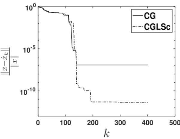
0 100 200 300 400 500 10-10 10-5 100 CG CGLSc

Fig. 1. \kappa (A) = 105. Relative error \| x - \^xk\| /\| x\| between the exact solution x and the computed

solution \^xkat iteration k for CG and CGLSc.

100 \times 50 rather than 40 \times 20). The condition number of the matrices is between 1 and 1010_{. The optimality measure considered is the relative solution accuracy \| x - \^}_{x\| /\| x\|} with x the exact solution (chosen to be x = [n - 1, n - 2, . . . , 0]T_{) and \^}_{x the} com-puted numerical solution. In the tests, c is chosen as a random vector of the form c = \=c rand(n, 1) for various choices of \=_{c \in \BbbR (cf. Table 1), and b = Ax - A}\dagger Tc. A simulation is considered unsuccessful if the relative solution accuracy exceeds 10 - 2.

5.2. Comparison of CGLS\bfitc with iterative methods. In this section, we compare the performance of CGLSc with the reference iterative methods. We first show its improved performance over CG on selected problems.

5.2.1. Solution accuracy. We first consider the numerical experiment corre-sponding to choice C1 with a = 0.5 , c = 10 - 1rand(n, 1), and \kappa (A) = 105_{. CG and} CGLSc are compared in Figure 1, where we report the relative error \| x - \^xk\| /\| x\| versus the number of iterations k. CG achieves an accuracy of order 10 - 7, while the error in the solution computed by CGLSc is \kappa (A) times smaller.

We now consider a second numerical experiment based on the choice C2 with up = 0.5, dw = 10 - \sanseight , c = 10 - 14rand(n, 1), and \kappa (A) = 5 \times 107_{, respectively. The gap} in the results is even larger: CGLSc finds an accurate solution, while CG does not solve the problem at all; see Figure 2.

We finally compare the two iterative methods plus MINRES on the synthetic set of matrices \scrP , where c is chosen as \=c rand(n, 1) for different values of \=c. We report in Figure 3 the performance profile corresponding to these simulations. MINRES has been applied to (1.1) for the two choices \xi = 1 and \xi = \xi \ast = \surd 1

2\sigma min(A) [3]. It is evident that a good scaling in (1.1) is beneficial for MINRES, but we also need to take into account that the computation of the optimal scaling parameter may be expensive. Clearly, CGLSc performs much better than CG and both versions of MINRES.

5.2.2. Forward error bounds. In this section, we wish to compare the clas-sical analysis for which the condition number of (ENE) is \kappa (A)2 _{and the backward} error for a computed solution \^x is \| AT_A\^_{x - A}T_{b - c\| /(\| A\|}2_{\| \^}_{x\| ), with the structured} analysis for which the relative condition number is given by \kappa S in (3.5) and the rel-ative (linearized) backward error is \=\eta r(\^x) := \=\eta (\^x, 1, 1)/\| (A, b, c)\| F, which is given in

(16)

0 20 40 60 80 100 120 10-10 10-8 10-6 10-4 10-2 100 CG CGLSc

Fig. 2. \kappa (A) = 5 \times 107. Relative error \| x - \^xk\| /\| x\| between the exact solution x and the

computed solution \^xk at iteration k for CG and CGLSc.

100 102 104 106 108 1010 0 0.1 0.2 0.3 0.4 0.5 0.6 0.7 0.8 0.9 1 CG CGLSc MINRES, =1 MINRES, = *

Fig. 3. Performance profile in logarithmic scale of CG, CGLSc, and MINRES on the synthetic set of matrices \scrP . MINRES is applied to (1.1) with \xi = 1 and \xi = \xi \ast _{. The optimality measure}

considered is the relative solution accuracy \| x - \^x\| /\| x\| with x the exact solution and \^x the computed numerical solution.

Lemma 3.5. For each analysis, the forward error \| x - \^x\| /\| x\| is predicted by the product of the condition number times the corresponding backward error, so that the classical bound will be \Delta C= \kappa (A)2\| ATA\^x - ATb - c\| /(\| A\| 2\| \^x\| ), and the structured one is \Delta S in (3.13).

In Table 2 we compare the two bounds with the forward error for different prob-lems of the form C1 and C2, for which we report the condition number of A and the relative structured condition number \kappa S. For all tests, the proposed first-order estimate provides an accurate upper bound for the forward error. On the contrary, the classical analysis gives a rather satisfactory precision when \kappa S \sim \kappa (A)2_{, but it} is too pessimistic in predicting the error in the case \kappa S \sim \kappa (A). In such cases the structured bound is much sharper than the standard bound. These results also show again that in general CGLSc performs better than CG.

(17)

0 100 200 300 400 500 10-16 10-14 10-12 10-10 10-8 10-6

Fig. 4. CGLSc, choice C1 with a = 2 and c = \sansr \sansa \sansn \sansd (\sansn , \sansone ). \| r - rk\| /(\| A\| \| x\| ) with r = b - Ax

and rkthe recurred residual defined in Algorithm 4.2 versus iteration index k with machine precision

\epsilon \approx 10 - 16_.

5.2.3. Norm of the residual. In Figure 4, we consider for CGLSc the quan-tity \| r - rk\| /(\| A\| \| x\| ) that appears in (4.3) (with r = b - Ax and rk defined in Algorithm 4.2). We can deduce that the bound (4.2) holds for k large enough, as (4.3) is satisfied with c1 = O(10); see Remark 4.2. This test corresponds to choice C1 with a = 2 and c = rand(n, 1), but the same behavior is observed in many other simulations.

5.3. Final comparison with direct methods. Motivated by practical ap-plications outlined in section 2, we have mainly focused on the design of iterative methods. However, it is also natural to consider direct methods for the solution of problem (ENE) that are known to be backward stable.

We consider two different methods:

\bullet QR, which solves (1.1) with \xi = 1, employing the QR factorization of [A, b] [2, 6], as described in Theorem 5.1 below.

\bullet AUG, which solves the augmented system (1.1) with \xi = \xi \ast _{using an LBL}T factorization [3]. We implement this method using the ldl MATLAB com-mand.

Theorem 5.1 (Theorem 1.3.3 [4]). Let A \in \BbbR m\times n, m \geq n, b \in \BbbR m, c \in \BbbR n. Assume that rank(A) = n and let

[A, b] = Q\biggl[ R d1 0 d2 \biggr]

. For any \xi \not = 0, the solution to (1.1) can be computed from

RTz = - c, Rx = (d1 - z), r = Q\biggl[ z d2

\biggr] .

We remark that the full orthogonal factor Q is required to compute r. Even if the QR factorization can be performed efficiently with Householder transformations,

(18)

Table 3

Summary of direct and iterative methods. We report the label used for the method, the formu-lation of the problem the method is applied to, and a brief description of each method.

Label Formulation Description

QR \biggl[ Im A AT 0 \biggr] \biggl[ r x \biggr] =\biggl[ b - c \biggr]

QR factorization of [A, b], Theorem 5.1

AUG \biggl[ \xi Im A

AT ₀

\biggr] \biggl[ \xi - 1_r

x \biggr] = \biggl[ b - \xi - 1_c \biggr]

LBLT, \xi = \xi \ast = \sigma min(A)/

\surd 2

CG AT_{Ax = A}T_{b + c} _{CG, Algorithm 5.1}

CGLSc AT_{Ax = A}T_{b + c} _{Modified CGLS, Algorithm 4.2}

MINRES \biggl[ \xi Im A

AT ₀

\biggr] \biggl[ \xi - 1_r

x \biggr] = \biggl[ b - \xi - 1_c \biggr]

Minimum residual method, \xi = 1, \xi = \xi \ast

100 101 102 103 0 0.1 0.2 0.3 0.4 0.5 0.6 0.7 0.8 0.9 1 AUG QR CGLSc

Fig. 5. Performance profile in logarithmic scale on the synthetic set of matrices \scrP considering CGLSc and the direct methods in Table 3. The optimality measure considered is the relative solution accuracy \| x - \^x\| /\| x\| with x the exact solution and \^x the computed numerical solution.

numerical experiments do not show a significant difference in the results using r = b - Ax.

All considered methods are summarized in Table 3. In Figure 5 we compare CGLSc with the direct methods on the same set of matrices used for the performance profile of Figure 3. Even if AUG and QR remain slightly more robust and more efficient, the performance of the proposed iterative method is really close to that of the two direct backward stable methods. The performance profile shows indeed that in about 70\% of the problems the difference in the solution accuracy is at most one digit and that in all cases it is at most three digits.

6. Conclusions. We considered both theoretical and practical aspects related to the solution of linear systems of the form (ENE). First, we studied the structured condition number of the system and proposed a related explicit formula for its com-putation. Then, we considered the numerical solution of (ENE). We found that the same issues that degrade the performance of the CG method on the normal equations also arise in this setting. This guided us in the development of a robust iterative method for solving (ENE), which has been validated numerically. From the

(19)

numeri-cal experiments, we can draw the following conclusions. The proposed method shows better performance than standard iterative methods in terms of solution accuracy. The error bounds proposed, based on structured condition numbers of the problems, are better able to predict forward errors than classical bounds from linear system the-ory. Finally, the solution accuracy achieved by the proposed method is comparable to that provided by stable direct methods.

Acknowledgments. The authors wish to thank Nick Higham, Theo Mary, and the anonymous referees for the really useful comments and suggestions that helped to improve the current version of the manuscript.

REFERENCES

[1] M. Arioli, M. Baboulin, and S. Gratton, A partial condition number for linear least squares problems, SIAM J. Matrix Anal. Appl., 29 (2007), pp. 413--433, https://doi.org/10.1137/ 050643088.

[2] A. Bj\"orck, Iterative refinement of linear least squares solutions I, BIT, 7 (1967), pp. 257--278, https://doi.org/10.1007/BF01939321.

[3] A. Bj\"orck, Pivoting and stability in the augmented system method, in Numerical Analysis

1991, Proceedings of the 14th Dundee Conference, D. F. Griffiths and G. A. Watson, eds., Pitman Res. Notes Math. 260, Longman Scientific and Technical, Essex, UK, 1992, pp. 1--16.

[4] A. Bj\"orck, Numerical Methods for Least Squares Problems, SIAM, Philadelphia, 1996.

[5] A. Bj\"orck, T. Elfving, and Z. Strakos, Stability of conjugate gradient and Lanczos methods

for linear least squares problems, SIAM J. Matrix Anal. Appl., 19 (1998), pp. 720--736, https://doi.org/10.1137/S089547989631202X.

[6] A. Bj\"orck and C. C. Paige, Loss and recapture of orthogonality in the Modified

Gram--Schmidt algorithm, SIAM J. Matrix Anal. Appl., 13 (1992), pp. 176--190, https://doi.org/ 10.1137/0613015.

[7] H. Calandra, S. Gratton, E. Riccietti, and X. Vasseur, On High-Order Multilevel Opti-mization Strategies, preprint, https://arxiv.org/abs/1904.04692 (2019).

[8] H. Calandra, S. Gratton, E. Riccietti, and X. Vasseur, On a multilevel Levenberg-Marquardt method for the training of artificial neural networks and its application to the solution of partial differential equations, Optim. Methods Softw., 2020, https://doi.org/ 10.1080/10556788.2020.1775828.

[9] X. W. Chang and D. Titley-Peloquin, Backward perturbation analysis for scaled total least-squares problems, Numer. Linear Algebra Appl., 16 (2009), pp. 627--648, https://doi.org/ 10.1002/nla.640.

[10] A. J. Cox and N. J. Higham, Backward error bounds for constrained least squares problems, BIT, 39 (1999), pp. 210--227, https://doi.org/10.1023/A:1022385611904.

[11] E. D. Dolan and J. J. Mor\'e, Benchmarking optimization software with performance profiles,

Math. Program., 91 (2002), pp. 201--213, https://doi.org/10.1007/s101070100263. [12] T. Elfving, On the Conjugate Gradient Method for Solving Linear Least Squares Problems,

Technical report, Department of Mathematics, Link\"oping University, Link\"oping, Sweden, 1978.

[13] R. Estrin, M. P. Friedlander, D. Orban, and M. A. Saunders, Implementing a smooth ex-act penalty function for general constrained nonlinear optimization, SIAM J. Sci. Comput., 42 (2020), pp. A1836--A1859, https://doi.org/10.1137/19M1255069.

[14] R. Estrin, D. Orban, and M. A. Saunders, LNLQ: An iterative method for least-norm problems with an error minimization property, SIAM J. Matrix Anal. Appl., 40 (2019), pp. 1102--1124, https://doi.org/10.1137/18M1194948.

[15] R. Fletcher, A class of methods for nonlinear programming: III. Rates of convergence, in Numerical Methods for Non-linear Optimization, Academic, London, 1972, pp. 371--381.

[16] V. Frayss\'e, S. Gratton, and V. Toumazou, Structured backward error and condition number

for linear systems of the type A\ast _{Ax = b, BIT, 40 (2000), pp. 74--83, https://doi.org/10.}

1023/A:1022366318322.

[17] V. Frayss\'e, S. Gratton, and V. Toumazou, Structured Backward Error and Condition

Num-ber for Linear Systems of the Type A\ast Ax = b, Technical report CERFACS TR/PA/99/05,

(20)

[18] A. J. Geurts, A contribution to the theory of condition, Numer. Math., 39 (1982), pp. 85--96, https://doi.org/10.1007/bf01399313.

[19] G. H. Golub and C. F. Van Loan, Matrix Computations, 4th ed., The Johns Hopkins Uni-versity Press, Baltimore, MD, 2012.

[20] S. Gratton, On the condition number of linear least squares problems in a weighted Frobenius norm, BIT, 36 (1996), pp. 523--530, https://doi.org/10.1007/BF01731931.

[21] A. Greenbaum, Estimating the attainable accuracy of recursively computed residual meth-ods, SIAM J. Matrix Anal. Appl., 18 (1997), pp. 535--551, https://doi.org/10.1137/ S0895479895284944.

[22] M. Hestenes and E. Stiefel, Methods of conjugate gradients for solving linear systems, J. Res. Natl. Bur. Standards, 49 (1952), pp. 409--436.

[23] N. J. Higham, Accuracy and Stability of Numerical Algorithms, 2nd ed., SIAM, Philadelphia, 2002, https://doi.org/10.1137/1.9780898718027.

[24] X. G. Liu and N. Zhao, Linearization estimates of the backward errors for least squares problems, Numer. Linear Algebra Appl., 19 (2012), pp. 954--969, https://doi.org/10.1002/ nla.827.

[25] J. Nocedal and S. J. Wright, Numerical Optimization, 2nd ed., Springer, New York, 2006, https://doi.org/10.1007/978-0-387-40065-5.

[26] C. C. Paige and M. A. Saunders, Solution of sparse indefinite systems of linear equations, SIAM J. Numer. Anal., 12 (1975), pp. 617--629, https://doi.org/10.1137/0712047. [27] C. C. Paige and M. A. Saunders, LSQR: An algorithm for sparse linear equations and sparse

least squares, ACM Trans. Math. Software, 8 (1982), pp. 43--71, https://doi.org/10.1145/ 355984.355989.

[28] J. R. Rice, A theory of condition, SIAM J. Numer. Anal., 3 (1966), pp. 287--310, https: //doi.org/10.1137/0703023.

[29] B. Walden, R. Karlson, and J. G. Sun, Optimal backward perturbation bounds for the linear least squares problem, Numer. Linear Algebra Appl., 2 (1995), pp. 271--286, https: //doi.org/10.1002/nla.1680020308.