Review of criteria for the selection of probability distributions for wind speed data and introduction of the moment and L-moment ratio diagram methods, with a case study.

1

Review of criteria for the selection of probability distributions for wind speed data

and introduction of the moment and L-moment ratio diagram methods, with a case

study

4

T.B.M.J. Ouarda1, 2*, C. Charron2 and F. Chebana1 5

6

1

INRS-ETE, National Institute of Scientific Research, 490 de la Couronne, Quebec City (QC), 7

Canada, G1K9A9 8

9

2

Institute Center for Water and Environment (iWater), Masdar Institute of Science and 10

Technology, P.O. Box 54224, Abu Dhabi, UAE 11 12 13 *Corresponding author: 14 Email: touarda@masdar.ac.ae 15 Tel: +971 2 810 9107 16 17 18 19 April 2016 20

2

Abstract

21

This paper reviews the different criteria used in the field of wind energy to compare the 22

goodness-of-fit of candidate probability density functions (pdfs) to wind speed records, and 23

discusses their advantages and disadvantages. The moment ratio and L-moment ratio diagram 24

methods are also proposed as alternative methods for the choice of the pdfs. These two methods 25

have the advantage of allowing an easy comparison of the fit of several pdfs for several time 26

series (stations) on a single diagram. Plotting the position of a given wind speed data set in these 27

diagrams is instantaneous and provides more information than a goodness-of-fit criterion since it 28

provides knowledge about such characteristics as the skewness and kurtosis of the station data 29

set. In this paper, it is proposed to study the applicability of these two methods for the selection 30

of pdfs for wind speed data. Both types of diagrams are used to assess the fit of the pdfs for wind 31

speed series in the United Arab Emirates. The analysis of the moment ratio diagrams reveals that 32

the Kappa, Log-Pearson type III and Generalized Gamma are the distributions that fit best all 33

wind speed series. The Weibull represents the best distribution among those with only one shape 34

parameter. Results obtained with the diagrams are compared with those obtained with goodness-35

of-fit statistics and a good agreement is observed especially in the case of the L-moment ratio 36

diagram. It is concluded that these diagrams can represent a simple and efficient approach to be 37

used as complementary method to goodness-of-fit criteria. 38

Keywords: wind speed; probability density distribution; moment ratio diagram; L-moments;

39

goodness-of-fit criteria; adequacy statistics. 40

3

1 Introduction

41

The assessment of wind energy potential at a given site is often based on the use of probability 42

density functions (pdfs) to characterize short term wind speed observations [1-16]. The selection 43

of the appropriate pdf to model wind speed data is crucial in wind power energy applications as 44

it reduces wind power output estimation uncertainties. Traditionally, the two-parameter Weibull 45

(W2) is the most used pdf in studies related to wind speed data analysis [17]. While being 46

extensively used in studies dedicated to the assessment of wind energy [18-25] , the Weibull is 47

not able to represent every wind speed regime [26-28]. Recently, a number of studies have used a 48

variety of other pdfs with variable levels of success [17, 22, 27-40]. The pdfs used include the 49

Gamma (G), Inverse Gamma (IG), Inverse Gaussian (IGA), two and three-parameter Lognormal 50

(LN2, LN3), Logistic (L), Log-logistic (LL), Gumbel (EV1), Generalized Extreme Value (GEV), 51

three-parameter Beta (B), Pearson type III (P3), Log-Pearson type III (LP3), Burr (BR), Erlang 52

(ER), Kappa (KAP) and Wakeby (WA) distributions. Ouarda et al. [27] found the GG and KAP 53

to be superior to W2 in the United Arab Emirates (UAE). Mert and Karakus [34] found the Burr 54

distribution to be more suitable than the GG or W2 for wind speed data in Antakya, Turkey. 55

A number of authors have proposed mixture distributions [13, 27, 28, 31, 41-46]. The mixture 56

models were found to provide better fit in the case of distributions presenting bimodal 57

characteristics. A model composed of two Weibull distributions is most often used [27, 31, 46-58

48]. Other mixture models used are the Normal-Normal, Truncated Normal-Weibull and 59

Gamma-Weibull. Shin et al. [28] applied a large number of different mixture models to wind 60

speed data in the UAE and concluded that the Weibull-Extreme value type-1 is the most 61

appropriate distribution. The use of distributions generated by the maximum entropy principle is 62

also common [13, 49-52]. These distributions have the advantage of being able to model wind 63

4

regime with high percentages of null wind speeds and with bimodal distributions [50]. Non-64

parametric models were also proposed by a number of authors to model wind speed distribution. 65

Qin [53] proposed to apply the kernel density concept to wind speed. This method was since 66

adopted in a number of studies [27, 35, 54, 55]. 67

Different goodness-of-fit criteria are traditionally used for the assessment of the adequacy of 68

pdfs. An exhaustive review of the most used criteria is presented in this paper along with a 69

discussion of their advantages and disadvantages. Such criteria include the log-likelihood (ln L) 70

[27, 33, 56, 57], the Akaike and the Bayesian Information Criteria (AIC, BIC) [27, 28, 30, 42, 71

56], the coefficient of determination ( 2

R ) [1, 3, 11, 12, 15-17, 21, 27, 28, 30-32, 35, 37, 39, 46, 72

49, 50, 58-62], the root mean square error (RMSE) [1, 2, 9, 13, 15, 16, 33, 36, 37, 39, 53, 56, 60-73

71], the Chi-square test statistic (2) [1, 2, 13, 15, 27, 28, 32-36, 39, 40, 49, 53, 55, 57, 60, 68, 74

72], the Kolmogorov-Smirnov test statistic (KS) [9, 13, 27, 30, 32-35, 38-40, 53, 55, 56, 61, 69, 75

73-75] and the Anderson-Darling test statistic (AD) [32, 40, 50, 76]. 76

An alternative method for the evaluation of the goodness-of-fit of pdfs, the moment ratio 77

diagram, has been used extensively in hydro-meteorology [77]. Bobée et al. [78] pointed out that 78

moment ratio diagrams have been used as a means to select a distribution to be used as a 79

probability model for the fitting of a given data sample, to compare the shapes of distributions 80

from a given set and to classify a set of distributions by separating them into a finite number of 81

categories. With this approach, all possible values of the square of the coefficient of skewness 82

and coefficient of kurtosis are represented in a coordinate system for each distribution. The 83

selection of the appropriate distribution to fit a data sample is made based on the location of the 84

data sample in the coordinate system. The main advantage of this approach is that it allows an 85

easy comparison of the fit of several pdfs on a single diagram. Moment ratio diagrams are also 86

5

easy to implement with the information and equations readily available in the literature, giving 87

the approximate relationship between moments for popular pdfs [79, 80]. The position of a time 88

series (i.e., a station) on the diagram is simply computed with the equations of moments. 89

The L-moment ratio diagram, a variant of the conventional moment ratio diagram, introduced by 90

Hosking [81], has been used to select suitable pdfs for modeling hydro-meteorological variables 91

in a large number of studies [79, 81-98]. Hosking and Wallis [79] presented the theoretical 92

advantages of L-moments over conventional moments: They are able to characterize a wider 93

range of distributions and they are more robust to the presence of outliers in the data when 94

estimated from a sample. They also indicated that experience shows that L-moments are less 95

subject to bias in estimation. Vogel and Fennessey [99] concluded that L-moment ratio diagrams 96

should be preferred over moment ratio diagrams for applications in hydrology. The main reason 97

is that L-moment estimators are nearly unbiased for all sample sizes and all distributions. 98

Despite its advantages, the moment ratio diagram approach has never been used for the 99

assessment of wind speed distributions. It is proposed, in the present study, to develop the 100

moment and L-moment ratio diagram approaches for wind speed data analysis and apply these 101

approaches to wind speed data from the UAE. Ouarda et al. [27] evaluated the suitability of a 102

wide selection of pdfs to fit wind speed data recorded at 7 stations at 10 m height in the UAE. 103

The adequacy of the pdfs was evaluated using goodness-of-fit criteria. For comparison purposes, 104

the same pdfs used in Ouarda et al. [27] for wind speed analysis are represented on the moment 105

ratio diagrams. These pdfs include the W2, W3, EV1, G, GG, GEV, LN2, LN3, P3, LP3 and 106

KAP. Both moment and L-moment ratio approaches are used and compared to the results 107

obtained from goodness-of-fit criteria. 108

6

The present paper is organized as follows: Section 2 reviews the different criteria of goodness-109

of-fit, found in the literature, for the assessment of probability distribution functions for wind 110

speed data. Section 3 presents the theoretical background on the conventional moment ratio 111

diagrams and the L-moment ratio diagrams. Section 4 presents the methodology used to 112

represent the selected pdfs on moment ratio diagrams. A case study dealing with the application 113

of moment ratio diagrams is presented in Section 5 and the results are presented in Section 6. 114

Finally, conclusions are given in section 7. 115

116

2 Review of the criteria used for the assessment of goodness-of-fit

A standard approach for the assessment of the goodness-of-fit is to visually compare the fit of the 118

candidate pdfs. For that, wind speed samples are usually divided into class intervals and 119

frequencies are represented with histograms. Candidate distributions are then superimposed on 120

the histograms. Alternatively, plots of the cumulative probability, P-P plots or Q-Q plots are also 121

represented. However, goodness-of-fit criteria provide an objective comparison of the candidate 122

distributions and are extensively used along with the visual approach. This section reviews the 123

criteria commonly used in the literature related to wind energy applications. 124

In general, the most used criteria are the ln L, AIC, BIC, R , 2 2

, KS, and AD. The KS, 2

and 125

AD statistics are associated to statistical tests that allow to identify if a sample is generated from 126

a given theoretical distribution. In the context of wind speed distribution assessment, the 127

statistics of these tests are used to compare the fit obtained by several theoretical distributions. 128

Alternatively, assessment of the fit is also based on the ability of the model to predict wind 129

power accurately. 130

7

2.1. Log-likelihood (ln L), and Akaike and Bayesian Information Criteria (AIC, BIC)

131

A given pdf f_ˆ( )x fitted on a wind speed data set has distribution parameter estimates



132

then defined by: 133







where v_i is the ith observed wind speed and n is the number of observations in the data set. A 135

higher value of this criterion indicates a better fit of the model to the data. 136

AIC [100] and BIC[101] are related to the log-likelihood and are defined by: 137













where k is the number of parameters of the distribution to estimate. A lower value of these 140

criteria indicates a better fit of the model to the data. These criteria take into consideration the 141

parsimony of the model as they include a penalty term that increases with the number of 142

parameters. For n 8, BIC provides a stronger penalty than AIC for additional parameters. 143

2.2. Coefficients of determination (R2)

144

R2 is a measure of how much the variance of the observed data is explained by the model. The 145

general form of R2 is given by: 146 2 2 1 2 1 ( ) 1 ( ) n i i i n i i y x R y y      





8

where y_i is the ith observed data, x_i is the ith predicted data and n is the sample size. 148

Alternatively, the square of the coefficient of correlation is also frequently used. 4 different 149

versions of this statistic are presented here. 150

2.2.1. R_PP2 151

2

PP

R is the coefficient of determination associated with the P-P plot defined by the model 152

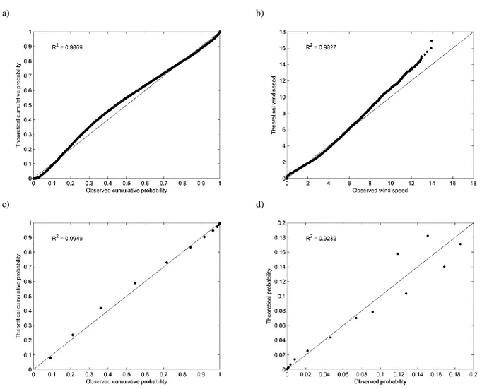
cumulative probabilities versus the empirical cumulative probabilities. An example of a P-P plot 153

is given in Fig. 1a. R_PP2 is computed as follows: 154 2 2 1 2 1 ˆ ( ) 1 ( ) n i i i PP n i i F F R F F      





where ˆF is the predicted cumulative probability of the ith observed wind speed, _i F is the i

156

empirical probability of the ith observed wind speed and F 1 _in₁Fi

n 





empirical probabilities, the Weibull plotting position is generally used: 158 ( ) 1 i i F v n   (6) 159

where i 1,...,n is the rank for ascending ordered observed wind speeds. This formula is 160

frequently used with P-P plots because it always gives an unbiased estimate of the empirical 161

cumulative probabilities regardless of the underlying distribution being considered [31]. Another 162

alternative is to use the Cunnane plotting position [102]: (v ) 0.4 0.2 i i F n    . 163 2.2.2. R_QQ2 164

9

2

QQ

R is the coefficient of determination associated with the Q-Q plot defined by the predicted 165

wind speed quantiles versus the observed wind speeds. An example of a Q-Q plot is given in Fig. 166

1b. The ith predicted wind speed quantile vˆ_i is given by vˆ_i F1(F_i), where F1( )x is the 167

inverse function of the theoretical cdf and F is the empirical probability of the ith observed i

168

wind speed. R_QQ2 is computed as follows: 169 2 2 1 2 1 ˆ ( ) 1 ( ) n i i i QQ n i i v v R v v      





where v is the ith observed wind speed and _i

1 1 n i i v v n  



For the following two R2 statistics, observed wind speed data are arranged in a relative frequency 173

histogram having N class intervals. R_{F c}2_, is the coefficient of determination measuring the fit 174

between the theoretical cdf and the cumulative relative frequency histogram of wind speeds. It is 175

similar to R_PP2 but is based on a histogram approach. An example of a P-P plot with histogram is 176

given in Fig. 1c. R_{F c}2_, is computed as follows: 177 2 2 1 , ₂ 1 ˆ ( ) 1 ( ) N i j i F c N i i F F R F F      





where ˆF_i is the predicted cumulative probability at the ith class interval, F is the cumulative _i 179

probability of relative frequencies at the ith class interval and

1 1 N i i F F N  



10 2.2.4 R_{p c}2_, 181 2 , p c

R is the coefficient of determination measuring the fit between the predicted probabilities at 182

the class intervals obtained with the theoretical pdf and the relative frequencies of the histogram 183

of wind speed data. An example of a graph representing the relation between these theoretical 184

and observed probabilities is given in Fig. 1d. R_{p c}2_, is computed as follows: 185 2 2 1 , ₂ 1 ˆ ( ) 1 ( ) N i i i p c N i i p p R p p      





where pˆ_i F v( _i)F v( _i1) is the estimated probability at the ith class interval, v_i₁ and vi are

187

the lower and upper limits of the ith class interval, p_i is the relative frequency at the ith class 188 interval and 1 1 N i i p p N  



In the R statistics presented above, the parsimony is not considered. These statistics tend 2 191

hence to favor more complex models, which use a larger number of parameters and provide 192

increased flexibility. The adjusted R , denoted 2 R , was developed to penalize the statistic for _a2 193

additional parameters. It is given by the following adjustment formula: 194 2 2 1 1 (1 ) a N R R N d      (10) 195

11

where R is anyone of the 2 R statistics presented above, d is the number of parameters in the 2 196

model and N is the wind speed sample size or the number of class intervals in the case of 197

statistics based on the histogram approach. 198

2.3. Root mean square error (RMSE)

199

The RMSE evaluates the difference between the observed and predicted values. It is generally 200

used either with predicted wind speed values (i.e.,

1/2 2 1 ˆ RMSE_v n ( _{i i}) / i v v n   _



predicted relative frequencies of the histogram of wind speed data, (i.e., 202 1/2 2 1 ˆ RMSE_p N ( _{i i}) / N i p p  

_



RMSE_p is associated with the graph in Fig. 1d. It is important to mention that the RMSE is 204

considered as an important performance index since it combines both the dispersion and the bias. It 205

can be shown for instance in the case of RMSEv (see [103]) that we have:

206

2 ( 1) 2 2

RMSE_v n STD_v bias_v n



  where STD_v is the standard error of the data and bias is the bias _v 207

of predicted wind speed values. 208

2.4. Chi-square test statistic (2 )

209

The Chi-Square test accepts or rejects the null hypothesis that the observed sample distribution is 210

consistent with a given theoretical distribution. The test statistic is first computed and a critical 211

value for the test is found at a given significance level. In the context of the assessment of model 212

distributions for wind speed data, the statistical value of the test is often used to compare the 213

goodness-of-fit of several theoretical distributions. To compute the Chi-Square test statistic, the 214

12

sample is arranged in a frequency histogram having N class intervals. The Chi-Square test 215

statistic is given by: 216







where O is the observed frequency in the ith class interval and i E is the expected frequency in i

218

the ith class interval. E is given by _i F v( )_i F v( _i1) where v_i₁ and vi are the lower and upper

219

limits of the ith class interval. A minimum expected frequency is usually required for each class 220

interval as an expected frequency that is too small for a given class interval will have too much 221

weight. When an expected frequency of a class interval is too small, it is usually combined with 222

the adjacent class interval. 223

2.5. Kolmogorov-Smirnov (KS) and Anderson-Darling (AD) test statistics

224

The KS and AD tests are also used to judge the adequacy of a given theoretical distribution for a 225

given set of observed wind speed data. Like the Chi-Square test in the context of the assessment 226

of model distributions to wind speed data, the values of the statistics of these tests are often used 227

to compare the goodness-of-fit of several theoretical distributions to the observed data. Both KS 228

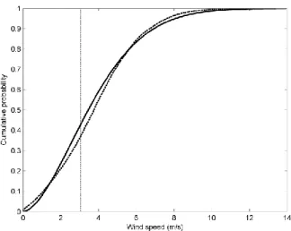
and AD statistics compare the cdf of the theoretical distribution with the empirical cumulative 229

probability distribution of wind speed data. Fig. 2 illustrates an example of both cumulative 230

distributions sketched together on the same plot. The KS test computes the largest difference 231

between the predicted and the observed distribution. The KS-test statistic is given by: 232 1 ˆ max _{i i} i n D F F     . (12) 233

13

where ˆF is the ith predicted cumulative probability from the theoretical cdf and _i F is the i

234

empirical probability of the ith observed wind speed. The AD [104] test statistic is defined by the 235 following equation: 236 2 ˆ ( ) ( ) ( ( )) ( ) A n F x F x  F x dF x     



where (x)_F xˆ( )(1F xˆ( ))_1 is a nonnegative weight function. Eq. (13) can be rewritten for 238

a finite data sample as: 239 1 1 2 1 _{ˆ ˆ} ln( ) ln(1 ) n i n i i i A n F F n      _{ }   _{ }   _ 



Because of the weight function, the AD test gives more weight to the tails of the distribution than 241

the KS test. 242

2.6. Advantages and disadvantages of the different methods

243

The methods presented above have different advantages and disadvantages. 2

PP

R , R_{F c}2_, , KS and 244

AD are related to the P-P plot. They are hence more sensitive to the middle part of the wind 245

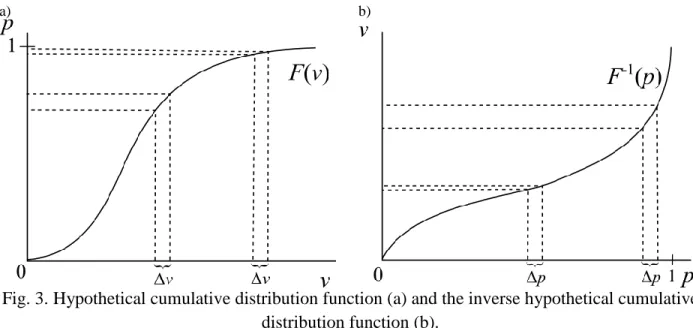
speed distribution where the gradient of the cumulative distribution function is the largest [105]. 246

Fig. 3a presents a graph of a hypothetical cdf showing the effect of small differences in wind 247

speed (v ) on the probabilities p. It can be seen that v in the middle part of the distribution 248

produces a larger variation in p than in the right tail. Because of the weight function involved in 249

the definition of the AD test, it is more sensitive to the tails of the distribution than KS. 250

14

2

QQ

R is related to the Q-Q plot. It is hence more sensitive to the tails of the distribution where the 251

gradient of the inverse cumulative distribution function is largest [105]. Fig. 3b presents a graph 252

of a hypothetical inverse cdf showing the effect of small differences in the percentile (p) on the 253

wind speed quantiles v. It can be seen that p in the right tail of the distribution produces a 254

larger variation in the quantiles than in the middle part. 255

The use of P-P plots is often preferred over the use of Q-Q plots because the Weibull plotting 256

position provides an unbiased estimate of the observed cumulative probabilities for the P-P plot 257

independently of the theoretical distribution considered [31, 32]. Ln L, AIC and BIC are also 258

more sensitive to the tails of the distributions. Indeed, the definition of these criteria includes the 259

sum of the logarithmically transformed densities of the observed wind speeds, and the magnitude 260

of the logarithmically transformed density is larger in the tails than in the middle part of the 261 distribution. 262 2 , p c R ,RMSE_p and 2

are associated with probabilities in class intervals. Because 2

is a 263

measure of the relative error in class intervals, it is more sensitive to the tails of the distribution 264

where the expected frequencies are small than R_{p c}2_, and RMSE_p. 265

The majority of the criteria discussed above do not take into account the parsimony of the 266

models. AIC, BIC and 2

a

R , on the other hand, penalize models that have a larger number of 267

parameters. The use of the adjusted

R

a

R ) is more relevant when the histogram approach is 268 adopted ( 2 , F c R , 2 , p c

R ). On the other hand, when no histograms are defined and the wind speed 269

data is used directly ( 2

PP

R , 2

QQ

R ), the adjusted

R

R

because of the large sample size usually available in wind speed analysis. Indeed, Eq. (10) shows 271

15

that when N is very large compared to d, we have 2 2

a

R R and the adjustment due to the number 272

of parameters is not significant. 273

Criteria that use the histogram approach (2, 2 ,

F c

R , Rp c2, and RMSEp) have the advantage of

274

being less affected by individual observations. However, the results depend on the subjective 275

choice of class intervals. 276

It is important to note that 2, KS and AD are commonly used in practice to evaluate if a given 277

theoretical distribution represents the parent distribution of a given data set. This is due to the 278

fact that these represent statistical tests with explicitly defined test critical values. The critical 279

values for 2 and AD depend on the theoretical distribution, while the critical value is 280

independent of the theoretical distribution for KS. 281

Finally, the values of the criteria

R

sample considered and thus these criteria can be used to compare the fit of different samples 283

(stations). This is not possible with criteria such as AIC or RMSE, as their values will differ 284

significantly from one data sample to another. These criteria can only be used to compare the fit 285

of different models for the same data set. 286

2.7. Wind power error

287

Celik [4] points out that in the field of wind engineering, wind speed distribution functions are 288

ultimately used to correctly model the wind power density. Therefore, the most important 289

criterion for the suitability of a possible wind speed distribution function should be based on how 290

successful it is in predicting the observed wind power density. For a given theoretical pdf

f v

( )

fitted on the wind speed data, the resulting wind power density distribution is given by: 292

16 3 1 ( ) ( ) 2 P v  v f v (15) 293

where ρ is the air density. The fit is often evaluated visually by plotting the estimated power 294

density distributions of the candidate pdfs along with the wind power density histogram obtained 295

from the observed wind speed data. The

R

used as objective criteria to measure the goodness-of-fit in these graphs [4, 15, 17, 21, 51, 66, 68, 297

69]. 298

Another popular approach involves comparing the mean wind power output [1, 13, 26, 31, 32, 299

65] (or the wind energy output [5, 21]) generated from the theoretical pdf with the mean wind 300

power output calculated from the observed wind speed data. The mean wind power density for 301

the theoretical pdf

f v

( )



The mean wind power density calculated from the observed wind speed data is given by: 304 3 0 1 2 P  v . (17) 305

Alternatively, a specific wind turbine is sometimes considered for the computation of the power 306

output. In that case the mean wind turbine power from the theoretical pdf and from the observed 307

wind speed data are given respectively by: 308 0 ˆ _{( ) ( )} w w P 



17 1 1 ( ) n w _i w i P P v n  



where P v is the power curve of the wind turbine. The difference between the theoretical _w( ) 311

power output and observed power output is often represented by the relative percent error: 312 ˆ 100 P P P     , (20) 313 where P P P₀( _w) and Pˆ P Pˆ ˆ₀( _w). 314 315

3 Theoretical background on moment and L-moment ratio diagrams

In the following, we present the mathematical background of conventional moment ratio 317

diagrams and L-moment ratio diagrams respectively. 318

3.1 Moment ratio diagram

319

Let us define a random variable X. The rth central moment of X is given by 320

( - ) ,r 2,3,...

r E X r

    , (21)

321

where





E X

( )





18

The 3rd and 4th moment ratios, also defined respectively as the coefficient of skewness (C ) S

324

and the coefficient of kurtosis (C ), are then _K 325 3 3 3/2 2 S C C









Moments are often computed from a data sample. Let us define x x₁, ₂,...,x , a data sample of _n 328

size n. The rth sample central moments are 329 1 1 ( ) , 2,3,... n r r i i m n x x r  







the coefficient of kurtosis are then respectively 332 3 3/2 2 ˆ S m C m  , (26) 333 4 2 2 ˆ K m C m  . (27) 334

Traditionally, moment ratio diagrams represent on a graph every possible value of ₁ in terms of 335

2

 where 2

1 CS

  and ₂C_K . Two-parameter distributions with a location parameter and a 336

scale parameter plot as a single point in the moment ratio diagram. Two and three-parameter 337

distributions with one shape parameter plot as a curve. Three and four-parameter distributions 338

19

with two or more shape parameters cover a whole area in the diagram. For all distributions, it can 339

be shown that the condition  ₂  ₁ 1 0 must be satisfied and thus an impossible region exists 340

in the diagram graph [106]. 341

Moment ratio diagrams can be used to select a pdf to model a given data sample. For this, the 342 sample estimates 2 1 ˆ ˆ S C

  and ˆ₂Cˆ_K are computed from the data sample and the point 343

1 2

ˆ ˆ

( ,

 

)

by comparing the position of this point with the theoretical pdfs represented on the moment ratio 345

diagram. 346

3.2 L-moment ratio diagram

347

L-moments, introduced by Hosking [81], are linear combinations of probability weighted 348

moments (PWM). They are analogous to the conventional moments. Let us define a random 349

variable X with a cumulative distribution function

F X

( )

x u

( )

were defined in Greenwood et al. [107] by the following expression: 351 , , [X {F(X)} {1 F(X) }] p r S p r s M E  . (28) 352

A useful special case of the PWM is B_r M_1,r,0 given by 353 1 0 [ { ( )} ]r ( ) r r B E X F X 



The L-moments of X are defined in Hosking [81] to be the quantities 355 1 , 0 r r r k k k p B





20 where 357 * , ( 1) r k r k r r k p k k        _{  }   . (31) 358

The dimensionless L-moment ratios, L-variation, L-skewness and L-kurtosis, are respectively 359 defined by 360 2 2 1 3 3 2 4 4 2 / / /             . (32) 361

L-moments possess an important property which makes them attractive for distribution fitting to 362

sample data and for the assessment of the goodness-of-fit: If the mean of the distribution exists, 363

then all L-moments exist and the L-moments uniquely define the distribution [79, 81]. 4 is

364

usually plotted against ₃ in L-moment ratio diagrams. As with conventional moment ratio 365

diagrams, the number of shape parameters determines if the pdf plots as a point, a curve or an 366

area in the diagram. 367

L-moments are often estimated from a finite sample. Let us define x_1:n x_2:n  x_n:n, an 368

ordered sample of size n. An unbiased estimator of the rth probability weighted moment B is _r 369 1 1 : 1 1 n 1 r j n j r n j b n x r r            _{   }  



The sample L-moments are defined by 371 1 , 0 , 0,1,..., 1 r r r k k k p b r n   



21

Analogously to Eq. (32), the sample L-moment ratios are defined by 373 2 2 1 3 3 2 4 4 2 / / / t t t    . (35) 374 375

4 Representation of probability distribution functions in moment ratio

diagrams

This section presents the methodology used to represent the selected pdfs in the moment and L-378

moment ratio diagrams. Table 1 presents the pdfs of all selected distributions with their domain 379

and number of parameters. For several pdfs, explicit expressions of ₂ as function of ₁ or ₄ as 380

function of ₃ are available in the literature in the form of polynomial approximations. These 381

expressions are then directly used to represent the points or curves. The expressions relating ₁ 382

and ₂ on one side, and ₄ and ₃ on the other sides, for the distributions EV1, GEV, G, P3, 383

LN2 and LN3 are given in Rao and Hamed [80] and Hosking and Wallis [79] respectively. They 384

also give the explicit expression for the bounds delineating the impossible regions. G and P3 on 385

one side and LN2 and LN3 on the other side have the same 3rd and 4th moment ratios, and are 386

hence represented by the same curve on the diagrams. The curve of the W2 distribution can be 387

obtained using the fact that ₃ and ₄ (or C and _S C ) for the W2 equal respectively _K ₃ and 388

4

 (or CS and C ) for the GEV. K

389

For pdfs that define areas (GG, LP3 and KAP), we are interested in defining the curves that 390

define the bounds of the areas. Analytical expressions of these curves are not available. The 391

22

relations between moments and distribution parameters are hence used and the numerical method 392

described below is applied. For a given pdf with three or four-parameters, let us define two shape 393

parameters h and k, and a position parameter μ and/or a scale parameter α. The 2nd and 3rd 394

moment ratios are independent of μ and α, and are hence given arbitrary values. Parameters h 395

and k are varied over a large range within the feasibility domain of the given pdf with small 396

intervals (h h h₁, ₂, ,h k_n; k k₁, ₂, ,k_m). For each possible pair (h k_i, _j), where h and _i k _j

397

are the ith and jth shape parameters, the corresponding pairs of moment ratios (_{1, ,i j},_{2, ,i j}) and ( 398

3, ,i j, 4, ,i j

  ) are obtained and are plotted on the moment ratio diagram and L-moment ratio 399

diagram respectively. This way, the contours of the regions defined by these points are found. 400

For most distributions, the shape parameters are unbound either in the positive or the negative 401

direction, and sometimes in both directions. This makes it impossible to explore the entire 402

feasibility domain of each parameter. However, for a given parameter, as its value becomes very 403

large or very small, points obtained in the moment ratio diagrams always converge to a limit 404

case. By using ranges with sufficiently extreme values for parameters in unbound directions, an 405

approximate area that accurately describes the feasible region is obtained. 406

The application of this method requires the use of the expressions relating moments and L-407

moments with distribution parameters. Bobée et al. [78] derived the expressions relating₁ and 408

2

 with the parameters of the GG and LP3 from the existing relation between noncentral 409

moments _rand distribution parameters and from the relation between central moments _r and 410

noncentral moments given in Kendall and Stuart [108]. This same approach is applied here 411

for the KAP distribution where the relation between and the distribution parameters are 412

found in Winchester [109]. The expressions of L-moment ratios ₃ and ₄ as functions of the 413

r



r

23

distribution parameters of the KAP are given in Hosking and Wallis [79]. However, explicit 414

expressions of L-moments in terms of the distribution parameters of the GG and LP3 are not 415

available. In this case, the values of B in Eq. (29) are solved by numerical integration. _r 416

Estimated B , ₁ B and ₂ B are then put in Eq. (30) to obtain ₃ ₂, ₃ and ₄ and subsequently ₃ 417

and ₄. 418

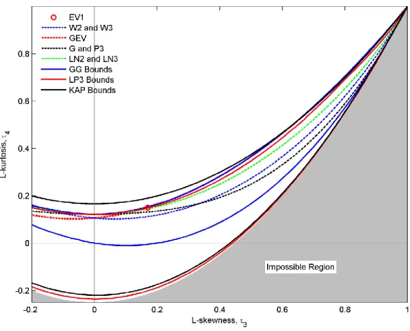
Figs. 4 and 5 present the moment ratio diagram and the L-moment ratio diagram obtained for the 419

selected pdfs of this study. These diagrams allow to analyze the flexibility of the different pdfs: a 420

pdf that can take on many different values of skewness and kurtosis is more flexible in terms of 421

shape of the distribution [77]. EV1 plots as a single point. Without any shape parameter, it has no 422

flexibility. It is a special case of the GEV. The GEV, W2-W3, G-P3 and LN2-LN3 distributions 423

having one shape parameter plot as lines. They are equivalent around zero skewness. G-P3 and 424

W2-W3 are special cases of the GG. The location parameter μ of LN2-LN3 also acts as a shape 425

parameter because of the logarithmic transformation on x. GG, LP3 and KAP plot as a whole 426

area. KAP is the most flexible followed by LP3 and GG. GG and KAP have 2 shape parameters. 427

The location parameter μ of LP3 also acts as a shape parameter because of the logarithmic 428 transformation on x. 429 430

5. Case study

The United Arab Emirates (UAE) is located in the south-eastern part of the Arabian Peninsula. It 432

is bordered by the Persian Gulf in the north, the Arabian Sea and Oman in the east, and Saudi 433

Arabia in the south and west. It lies approximately between 22°40’N and 26°N and between 434

24

51°E and 56°E. The total area of the UAE is about 83,600 km2. It can be divided into three 435

ecological areas: the northeastern mountainous area, the sandy/desert inland area and the marine 436

coastal area. The desert covers 80% of the country. The climate of the UAE is arid with very 437

high temperatures during summer. The coastal area has a hot and humid summer with 438

temperatures and relative humidity reaching 46 °C and 100% respectively. During winter, 439

temperatures are between 14 °C and 23 °C. The interior desert region has hot summers with 440

temperatures rising to about 50 °C and cool winters during which the temperatures can fall to 441

around 4 °C [110, 111]. 442

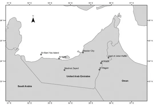
The Wind speed data used in this study comes from 7 meteorological stations located throughout 443

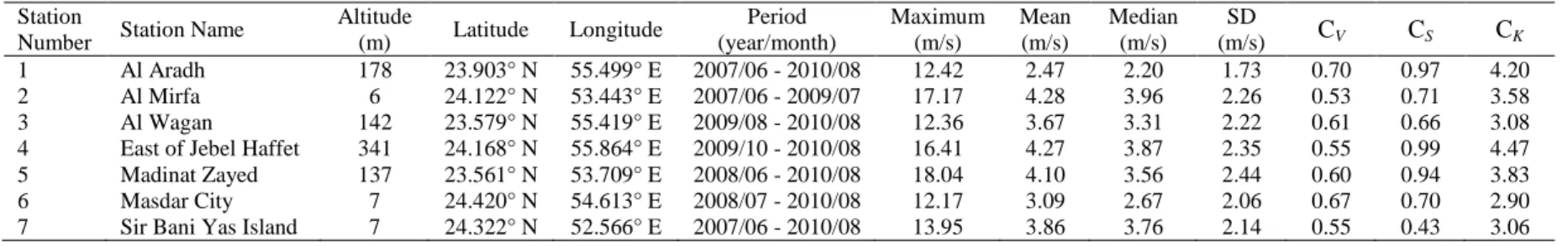
the UAE. Anemometers are at the 10 m height for all stations. Table 2 gives a description of the 444

stations including geographical coordinates, altitude, period of record, and wind speed statistics 445

including maximum, mean, median, standard deviation, coefficient of variation, coefficient of 446

skewness and coefficient of kurtosis. Periods of record range from 11 months to 39 months. A 447

map indicating the location of the stations is given in Fig. 6. The whole geographical region of 448

the UAE is well represented by these stations: The stations of Sir Bani Yas Island, Al Mirfa and 449

Masdar city are located near the coastline, the station of East of Jebel Haffet is located in the 450

mountainous north-eastern region, the station of Al Aradh is location in the foothills and the 451

stations of Al Wagan and Madinat Zayed are located inland. The inter-annual variability and the 452

long term evolution of wind speed data in these stations was studied by Naizghi and Ouarda 453

[112]. 454

Wind speed data used in this study was collected by anemometers at 10-min intervals. Average 455

hourly wind speed series, which is the most common time step used for characterizing short term 456

wind speeds, were then computed from the 10-min wind speed series. The resulting hourly wind 457

25

speed data can theoretically contain null values, as periods of calm can possibly last more than 458

one hour. For pdfs having a null probability of observing null wind speed, this would make it 459

impossible to estimate the distribution parameters with some methods. Therefore, any null values 460

are removed from the hourly data series of this study. The impact of removing null values was 461

checked to be insignificant as observed percentages of calms in the hourly time series are 462 marginally low. 463 464

6. Results

Sample moments and sample L-moments were computed for each wind speed series with Eqs. 466

(26) and (27), and Eq. (32) respectively. Wind speed samples were plotted in the moment ratio 467

diagram and the L-moment ratio diagram. These diagrams are presented in Figs. 7 and 8 468

respectively. Each station is numbered according to its rank in Table 2. The analysis of the 469

diagrams leads to the following conclusions about the suitability of the pdf to fit the stations 470

sample data. The curve of the W2-W3 passes through the middle of the cloud of points defined 471

by the samples. The G-P3, GEV and LN2-LN3 are located rather in the margin of the cloud of 472

points and are consequently not suitable to fit wind speed data. This makes W2-W3 the most 473

suitable pdf with one shape parameter for wind speed data in the UAE. However, some station 474

samples, such as stations 4 and 6, might be located far from the curve of the W2-W3. 475

Alternatively, all station samples are located within the regions bounded by GG, LP3 and KAP. 476

The selected pdfs were fitted to the wind speed data corresponding to all stations of this study. 477

The methods used for the estimation of the parameters of each pdf are also listed in Table 1. For 478

the majority of the distributions, the maximum likelihood method (ML) and/or the method of 479

26

moments (MM) were used. For KAP, the method of L-moments (LM) was used instead of MM. 480

The algorithm used for estimating the parameters with LM was proposed by Hosking [113]. For 481

the LP3, the Generalized Method of Moments (GMM) [114, 115] is used. 482

Each candidate distribution/method (D/M), a combination of a distribution with an estimation 483

method from Table 1, was fitted to the wind speed series presented in the case study. The 484

following criteria of goodness-of-fit were then calculated: ln L, 2 , F c R , 2 , p c R , 2, KS and AD. 485

For the coefficients of determination 2 ,

F c

R and 2 ,

p c

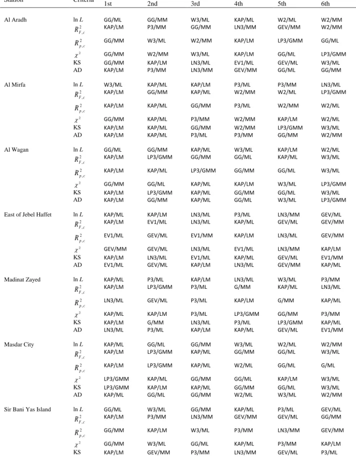
R , the adjusted version is considered. Table 3 486

lists the 6 best pdfs based on the goodness-of-fit criteria. In Fig. 9, each criterion except ln L is 487

presented with box plots representing the various D/Ms for all stations combined. For each 488

distribution, the D/M with the method leading to the best fit is represented. LN2 leading to 489

generally very poor fits was discarded from these box plots. 490

The conclusions obtained from the moment ratio diagrams are in general in agreement with those 491

obtained with the analysis of goodness-of-fit criteria. According to 2 ,

F c

R , KAP is by far the best 492

pdf followed by GG and LP3. According to 2 ,

p c

R , GG followed by KAP and LP3 are the best 493

pdfs. GG, W3 and KAP are, in this order, the best pdfs with respect to the 2 statistic, while 494

KAP, GG and LP3 are, in this order, the best pdfs with respect to the KS statistic. According to 495

AD, KAP and LP3 are the best pdfs. Based on the ranks obtained in Table 3 for ln L, KAP is the 496

best pdf followed in order by GG and W3. KAP is more flexible and is listed among the best 497

D/Ms for all 7 stations while GG is not included among the best pdfs for the stations of Al Mirfa, 498

East of Jebel Haffet and Madinat Zayed. 499

Box plots reveal that the W2 is the best two-parameter distribution and leads to better 500

performances than several three-parameter distributions including the GEV, LN3 and P3. 501

27

According to most criteria, LP3 gives inferior fit than GG. This is surprising considering the 502

location of the samples which are within the area covered by the pdf. This point will be further 503

discussed below. 504

The relations between the location of individual stations on the moment and L-moment ratio 505

diagrams and the results obtained with the goodness-of-fit criteria are investigated. The analysis 506

of the conventional moment ratio diagram (Fig. 7) reveals the following: For Station 6, located 507

far from all curves, KAP, GG and LP3, which are pdfs that define regions, are preferred with 508

respect to all criteria. Furthermore, the clear outlier for P3/MM in the box plots of 2 , c

F

R and Rp c2,

509

corresponds to Station 6. Station 7 is close to the GEV curve in the diagram and this distribution 510

received generally good ranks for this station. On the other hand, Station 4 is right on the G-P3 511

curve but these pdfs are not particularly higher ranked for this station. 512

In the L-moment ratio diagram (Fig. 8), the following can be observed: Stations 1, 2 and 7 are 513

very close to the W2 curve. The ranks of the W2 or W3 for these stations are generally higher 514

than those of the other stations. Station 6 is also located far from the curves of the pdfs in this 515

diagram. Station 4 is located near the border of the region delineated by GG and LP3. This is in 516

agreement with the goodness-of-fit criteria which indicate that the GG and LP3 do not perform 517

very well for all criteria. Station 4 is also located very close to the curve of the GEV and the 518

point corresponding to EV1. These pdfs perform much better for this station while they perform 519

poorly for the others. Station 5, is located near the G-P3 curve. The goodness-of-fit criteria 520

obtained for this station are generally excellent. 521

In Fig. 10, the wind speed frequency histograms corresponding to each station are presented. The 522

pdfs of the W3/ML, GG/MM, LP3/GMM and KAP/LM are superimposed over these plots. 523

28

These plots allow to visualize and validate the fit obtained by the selected distributions. The 524

distribution parameters of the selected pdfs for each station are presented in Table 4. The KAP 525

distribution gives generally the best fit. In the case of station 1, no distribution was able to model 526

the lower part of this particular shape of histogram. This distribution presents a bimodal 527

behavior. This case illustrates the limitation of classical models in the presence of bimodality. 528

W3 fails to model adequately the distribution of East of Jebel Haffet and Masdar City (4 and 6 529

respectively). Consistently, stations 4 and 6 are located far from the W2-W3 theoretical curve in 530

the moment ratio diagrams. For East of Jebel Haffet and Madinat Zayed (stations 4 and 5 531

respectively), the pdfs of W3 displayed on the histograms underestimate the probability density 532

in the part of the distribution with the higher frequencies. Consistently, the locations of these 533

stations in the L-moment ratio diagram indicate that each sample data has a higher kurtosis than 534

the theoretical distribution of W2-W3 for a given skewness. In the conventional moment ratio 535

diagram, this consistency is not well observed as the location of station 5 indicates that the 536

observed data for that station have a lower kurtosis than the theoretical distribution of W2-W3 537

for the same skewness. 538

These results indicate that the goodness-of-fit criteria are more consistent with the results 539

obtained with the L-moment ratio diagram than with the conventional moment diagram. Indeed, 540

the location of individual stations in the L-moment ratio diagram allows drawing more 541

conclusions in agreement with the results obtained with the majority of the goodness-of-fit 542

criteria. This is in agreement with previous studies in the field of hydro-meteorology, where the 543

L-moment ratio diagram instead of the conventional moment ratio diagram was recommended. 544

Hosking [81] suggested the use of the L-moment ratio diagram especially for small size samples 545

because L-moment estimators are less biased than conventional moment estimates. Vogel and 546

29

Fennessey [99] found that conventional moment estimators are also biased for large samples 547

from highly skewed distributions. 548

As presented in the literature review, the model distributions are also often evaluated for their 549

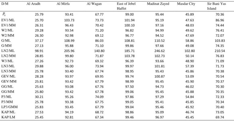
ability to model the average wind power. A comparison of the model distributions is also 550

presented herein using this criterion. The mean power density is computed using Eq. 17 and the 551

mean power densities for the theoretical distributions are computed using Eq. 16. Table 5 552

presents the mean power density obtained for the observed data and from the theoretical 553

distributions. The D/Ms that provide the best fits are LP3/GMM, P3/MM, GG/MM, GEV/MM, 554

LN3/MM and KAP/LM. These results are somewhat different from those obtained with the other 555

criteria. Indeed the GEV and LN3 distributions which lead to good results with the average wind 556

power criterion did not lead to equivalent performances with the other criteria. Fig. 11 presents 557

the wind power density frequency histogram for each station. Similarly to Fig. 10, the 558

distributions for the W3/ML, GG/MM, LP3/GMM and KAP/LM are superimposed over these 559

plots. 560

561

7. Conclusions and future work

In this study, a review of the various criteria used in the field of wind energy was presented, 563

along with a discussion of their advantages and disadvantages. The methods of moment ratio and 564

L-moment ratio diagrams were used for the assessment of pdfs to fit short term wind speed data 565

samples. These methods, often used in hydro-meteorology, offer a viable alternative to 566

goodness-of-fit tests and criteria commonly used for the analysis of wind speed data. Their main 567

advantage is that they allow an easy comparison of the fit of several pdfs on a single diagram. 568

30

They are also easy to implement and the position of the time series on the diagrams are easily 569

computed with the moment equations. 570

Diagrams for the conventional moment ratios and for the L-moment ratios were built for a 571

selection of 11 pdfs. For most pdfs defining a curve, expressions of ₂ in terms of ₁ or ₄ in 572

terms of ₃ are available in the literature. This allows a straightforward representation of curves 573

in the moment ratio diagrams. However, for pdfs with two shape parameters (KAP, GG and 574

LP3), an area is instead covered in the moment ratio diagrams and analytical expressions relating 575

the moment ratios to the limits of the areas are generally not available in the literature. An easy 576

numeric procedure is used to define the limits of these areas. Plotting the position of a given 577

wind speed data set in these diagrams is instantaneous and provides more information than a 578

goodness-of-fit criterion since it provides knowledge about such characteristics as the skewness 579

and kurtosis of the station data set. These diagrams have also the advantage of allowing an easy 580

comparison of the fit of several pdfs for several stations on a single diagram. 581

The method of moment ratio diagrams was applied here to a study case consisting of short term 582

wind speed data recorded in the UAE. Moment ratio diagrams were used to evaluate the 583

suitability of several pdfs to fit wind speed data. The conclusions based on the moment ratio 584

diagrams are as follows: Compared to other pdfs having one shape parameter and thus defining a 585

curve on the moment ratio diagram, W2 or W3 have the most central position with respect to 586

sample coordinates and should be considered as the best choice among these pdfs. However, 587

some samples could be located far from this curve. The pdfs with two shape parameters, GG, 588

LP3 and KAP, cover an area that encompasses every sample. KAP is the most flexible 589

distribution and hence its area covers the largest part of the diagrams. 590

31

Conclusions obtained with the diagrams were compared to results obtained with goodness-of-fit 591

criteria. It was observed that a better agreement exists between the conclusions drawn from 592

goodness-of-fit criteria and those from the L-moment ratio diagram, than those from the 593

conventional moment ratio diagram. This is in agreement with the theoretical advantages of the 594

L-moments and the results of the previous studies which concluded that L-moment ratio 595

diagrams should be used instead of conventional moment ratio diagrams. It is concluded that 596

these diagrams can represent a simple and efficient approach to be used in association with 597

commonly known goodness-of-fit criteria. 598

Classical frequency analysis tools used in wind speed modeling are based on the hypothesis of 599

temporal stationarity of the wind speed data. In reality, such assumption is not always met. A 600

considerable amount of research dealt with the development of non-stationary frequency analysis 601

procedures for hydro-climatic variables (see for instance [116, 117]). Future work should focus 602

on the use of non-stationary frequency analysis techniques for the modeling of wind speed series 603

in various regions around the globe. Moment ratio diagrams have never been used in the non-604

stationary context and can be adapted easily to analyze the temporal evolution of wind speed 605

characteristics. It is possible for instance to study the evolution of the position of a given sample 606

in the moment or L-moment ratio diagrams by considering a moving window through the data 607 series. 608 609

Acknowledgements

The authors wish to thank Masdar Power for having supplied the wind speed data used in this 611

study. The authors wish to express their appreciation to Dr. Mohamed Al-Nimr, Editor in Chief,

32

Dr. Nesreen Ghaddar, Editor, and three anonymous reviewers for their invaluable comments and

613

suggestions which helped considerably improve the quality of the paper.

614 615

33

Nomenclature

B rth probability weighted moment where M_1,r,0

618 1  moment ratio C_S2 619 2  moment ratio C _K 620 CV coefficient of variation 621 CS coefficient of skewness 622 CK coefficient of kurtosis 623

cdf cumulative distribution function 624

2

 Chi-square test statistic 625

D/M distribution/method 626

EV1 Gumbel or extreme value type I distribution 627

ˆ( )

f_ probability density function with estimated parameters ˆ 628

ˆ( )

f estimated probability density function 629

i

F empirical probability for the ith wind speed observation 630

ˆ

i

F estimated cumulative probability for the ith observation obtained with the theoretical 631

cdf 632

( )

F cumulative distribution function 633

1

( )

F inverse of a given cumulative distribution function 634

34 G Gamma distribution

635

GEV generalized extreme value distribution 636

GG generalized Gamma distribution 637

GMM generalized method of moment 638

KAP Kappa distribution 639

KS Kolmogorov-Smirnov test statistic 640 1 r sample rth L-moment 641 LM Method of L-moments 642

LN2 2-parameter Lognormal distribution 643

LN3 3-parameter Lognormal distribution 644

LP3 Log-Pearson type III 645 ML maximum likelihood 646 MM method of moments 647 r  rth central moment 648

n number of wind speed observations in a series of wind speed observations 649

N number of bins in a histogram of wind speed data 650

i

p the relative frequency at the ith class interval 651

ˆ_i

p the estimated probability at the ith class interval 652

0

ˆ

P mean wind power density for the theoretical pdf

f v

( )

0

P mean wind power density calculated from the observed wind speed data 654

35 ˆ

w

P mean wind turbine power from the theoretical pdf

f v

( )

w

P mean wind turbine power from the observed wind speed data 656

P3 Pearson type III distribution 657

pdf probability density function 658 2 R coefficient of determination 659 2 a R adjusted R 2 660 2 PP

R coefficient of determination giving the degree of fit between the theoretical cdf and the 661

empirical cumulative probabilities of wind speed data. 662

2

QQ

R coefficient of determination giving the degree of fit between the theoretical wind speed 663

quantiles and the wind speed data. 664

RMSE root mean square error 665

r

m rth sample central moment 666

, ,

p r s

M probability weighted moment of order p, r, s 667

r

 rth L-moment ratio 668

r

t rth sample L-moments ratio 669

i

v the ith observation of the wind speed series 670

ˆ_i

v predicted wind speed for the ith observation 671

W2 2-parameter Weibull distribution 672

W3 3-parameter Weibull distribution 673

36 674