Manuscript Details
Manuscript number AGWAT_2018_682_R1
Title DEVELOPMENT OF A STEADY-STATE MODEL TO PREDICT DAILY WATER
TABLE DEPTH AND ROOT ZONE SOIL MATRIC POTENTIAL OF A CRANBERRY FIELD WITH A SUBIRRIGATION SYSTEM
Article type Research Paper
Abstract
Maintaining a steady water table depth (WTD) to ensure an optimal soil matric potential in the root zone (RMAP) is vital when growing cranberry under a subirrigation system; owing to losses and other hydrological processes. The excessive rising or falling of the WTD may threaten the plant transpiration either by saturation or lack of moisture in the root soil. A steady-state model was developed for a uniform soil column to predict WTD and RMAP under different weather conditions. The model is based on van Genuchten (VG) and Brooks and Corey (BC) analytical soil water retention functions coupled with Mualem, Brooks and Corey, and Gardner hydraulic conductivity models. The results show that the model is capable of predicting satisfactorily both WTD and RMAP. The VG model performed with a 78.13% accuracy for the WTD and an 88.59% precision according to the Kling Gupta Efficiency coefficient (r2=0.90, β=1.00, and γ=0.99) for the field storage. Meanwhile for the RMAP the Mualem and Gardner hydraulic conductivity models, predictions were successful 71.87% and 75.00% of the time, respectively. The BC model had a 78.13% success for the WTD, 86.93% accuracy in estimating the field water storage according to Kling-Gupta efficiency coefficient (r2=0.89, β=1.00, and γ=1.00) and the BC and Gardner hydraulic conductivity models had 65.63% and 71.88% success, respectively. A sensitivity analysis of the model, by means of the Morris method, reveals that for both models, the lower boundary condition impacts significantly both variables which are, however, less affected by the field capacity and the residual soil moisture content. The lower boundary condition interacts with the slope of the soil water retention functions, the height of the capillary fringe, the saturated conductivity, and the saturation moisture content which have non-linear effects. An uncertainty analysis shows that both variables for both models are normally distributed.
Keywords evapotranspiration; soil water retention; van Genuchten; Brooks and Corey; Mualem; Gardner
Taxonomy Agriculture, Environmental Science
Corresponding Author Alain Rousseau Corresponding Author's
Institution
Institut national de la recherche scientifique Order of Authors Yao Bigah, Alain Rousseau, silvio gumiere Suggested reviewers Roger MOUSSA, jan Hopmans, Peter Troch
Submission Files Included in this PDF
File Name [File Type]
Submission_Letter.pdf [Cover Letter]
ANSWERS TO REVIEWERS COMMENTS_Final.docx [Response to Reviewers]
Bigah_Rousseau_Gumiere_With_track_changes.DOCX [Revised Manuscript with Changes Marked] HIghlights.docx [Highlights]
Bigah_Rousseau_Gumiere_Final.docx [Manuscript File] Fig1.tif [Figure] Fig2.tif [Figure] Fig3.tif [Figure] Fig4.tif [Figure] Fig5.tif [Figure] Fig6.tif [Figure] Fig7.tif [Figure]
To view all the submission files, including those not included in the PDF, click on the manuscript title on your EVISE Homepage, then click 'Download zip file'.
Research Data Related to this Submission
There are no linked research data sets for this submission. The following reason is given: The data that has been used is confidential
Institut national de la recherche scientifique
Centre - Eau Terre Environnement
490, rue de la Couronne
Québec City, December 11, 2018
Dr. Droogers Editor in Chief
Agricultural Water Management
Subject: Submission of a revised version of manuscript AGWAT_2018_682
Dear Editor in Chief,
Yao Bigah, Silvio J. Gumiere, and I would appreciate if you could consider for publication in
Agricultural Water Management the revised version of the following research paper entitled
“DEVELOPMENT OF A STEADY-STATE MODEL TO PREDICT DAILY WATER TABLE DEPTH AND ROOT ZONE SOIL MATRIC POTENTIAL OF A CRANBERRY FIELD WITH A SUBIRRIGATION SYSTEM”. All the reviewers’ comments and suggestions were incorporated in this revised version.
You will find in this submission: a document providing our responses to the reviewers’ comments, a revised manuscript without track changes, and finally a revised version of the manuscript with track changes. The content of the paper represents original work and has not been published or submitted elsewhere.
The major contributions and findings of this article are: (i) a steady-state model for a uniform soil column to predict water table depth (WTD) and soil matric potential in the root zone (RMAP) under different weather conditions was developed and successfully validated; (ii) the model is based on van Genuchten (VG) and Brooks and Corey (BC) analytical soil water retention functions coupled with Mualem, Brooks and Corey, and Gardner hydraulic conductivity models; (iii) a sensitivity analysis of the model, by means of the Morris method, reveals that for both models, the lower boundary condition impacts significantly WTD and RMAP which are, however, less affected by the field capacity and the residual soil moisture content; and (iv) an uncertainty analysis shows that WTD and RMAP for both models are normally distributed.
We hope that you will find the manuscript suitable for publication in the Journal of Agricultural
Water Management. We look forward to hearing from you soon.
Sincerely,
Alain N. Rousseau Ph.D., P. Eng. Professor-researcher
ANSWERS TO REVIEWERS COMMENTS
Reviewer 1 : Interesting paper. No specific comments Reviewer 2 :
1. Eq1 equation needs to be redefined because it seems that the horizontal flow of the water is not included.
Due to the configuration of cranberry fields (Figure 1.a) there is no horizontal flow as the fields are bordered by embankments which prevent surface water to run off the field. Moreover, the subirrigation channels bordering the field prevent losses through the field lateral frontier as the water level in the channel matches that of the cranberry field. So, surface water entirely infiltrates and reaches the water table. Such vertical flow is governed by the 1-D Richards equation representing the core of Eq.1.
Indeed, there is no horizontal flow except through the field subsurface drainage system represented by a sink term. So Eq. 1 is correctly written. Therefore, the following sentence: ‘The flow of water in such medium is expressed as a coupled, saturated-unsaturated and vertical-horizontal flow equation (Equation 1)’ becomes ‘The flow of water in such medium is expressed as a coupled, saturated-unsaturated and vertical flow equation (Equation 1)’
2. Many of the proposed formulas do not need to be inserted in the article because they are in all sources, such as 13 to 18.
The comment is relevant. Equations 13 to 18 are shifted into an appendix and the numbering of the rest of the Equations is reset.
3. Soil hydraulic conductivity (K) and capillary length (Lcap)
The soil capillary length (Lcap) is just a K-weighted mean soil-water potential as observed by
Raats and Gardner (1971). The sentence :
Elsewhere, for the unsaturated soil constricted between the water table depth and the soil surface, the White et al. (1987) capillary length approach is used to assess the macroscopic capillary length, 𝐿𝑐𝑎𝑝 [cm] (Equation 8) as well as the mean unsaturated hydraulic conductivity (Equation 9).
Is rephrased as follows:
For the unsaturated soil constricted between the water table depth and the soil surface, the ‘mean’ height of capillary rise above the water table, 𝐿𝑐𝑎𝑝 [cm] is assessed by means of Equation 8 (White et al. 1987) called the K-weighted mean soil water potential by Raats and Gardner (1971). As for the soil mean hydraulic conductivity, it is computed using Equation 9.
4. Due to the importance of hydraulic conductivity of the calculations and its measurement with other methods is controlled.
The soil hydraulic conductivity is measured using the constant head method on soil samples using a 5.7-cm diameter by 5.7-cm high cylinder.
5. This formula need to check" 𝐾(𝑆𝑒) =
𝐾𝑠𝑆3 + 2/𝜆𝐵𝐶". It is possible?
We are not sure to which equation this comment applies, but we infer it is to Eq. 6, which is now rewritten as follows: (6) 𝐾(𝑆𝑒)= 𝐾𝑠𝑆 3 + 2 𝜆𝐵𝐶 𝑒
This equation is well known as the Brooks and Corey (1964) soil hydraulic conductivity function. The Equation is correctly written as shown below from the reference paper:
Brooks, R.H., Corey, A.T., 1964. Hydraulic properties of porous media and their relation to drainage design. Trans. ASAE, 7(1): 26-0028.
6. Boundary conditions present clearly. Given the farm conditions, it does not match what is said. The site conditions are shown in Figure 1(a) & (b) and described in the text.
The boundary conditions match the farm conditions:
- The field surface is subjected to infiltration (from rainfall or irrigation) and plant evapotranspiration (Eq. 13)
- There is no runoff due to the protection of the field by embankment
- Uncontrolled minor losses through the subirrigation/drainage pipes (deep percolation) occur (Eq. 14);
- Surrounding channels ensuring the field subirrigation curb the lateral flow of water off the field, this justifies the zero-flux boundary condition on the lateral faces.
7. Why runoff, is negligible.Eq.19 with regard to whether and soil condition?
Cranberry fields are constructed farms which are protected by surrounding embankments preventing any surface water to exit the field by running off (Figure 1.a). So, water from weather conditions and irrigation infiltrates entirely into the field.
Indeed, we did not use one single ready-made model to compute the cranberry field water table depth (WTD) and root soil matric potential (RMAP). Well-known equations developed by
several authors were used, but they could not be used solely to provide solution to our problem. So we did design the way to put these pieces of equations together so that we could address the objectives of this paper. We think, it is a model development.
9. The problem has not been well addressed and what the problem really is to solve the problem. Goal of the work:
The goal of this paper is to use a mathematical model to simulate the hydrological processes in a cranberry field system in order to predict the fluctuation of the water table depth (WTD) as well as the root soil matric potential (RMAP) which could be used for irrigation management.
Is the problem solved?
- Mathematical equations are put together to build a single model;
- The model calculates satisfactorily cranberry field WTD and their RMAP; - The model is validated using data from field experiments;
- The sensitivity analysis of the model reveals the most and least influential parameters and the ensuing uncertainty analysis shows that the output are normally distributed.
The model can be used to predict cranberry field WTD and their RMAP for the betterment of irrigation scheduling; The objectives are achieved.
10. Due to the sensitivity of the model, some parameters have not been specified for simulating the necessary attention
Most sensitive parameters
- The lower boundary condition is found to be the most influential parameter for both variables, WTD and RMAP
- The less influential parameters are found to be the field capacity and the residual soil moisture content
11. In general, the article is good and can be printed in the journal but needs to be reviewed and some formulas are deleted and the data monitored. For complete
We would like to thank the reviewer for the time spent reviewing the paper and providing useful comments. Formulas 13 to 18 have been moved to the appendix
DEVELOPMENT OF A STEADY-STATE MODEL TO PREDICT
DAILY WATER TABLE DEPTH AND ROOT ZONE SOIL MATRIC POTENTIAL OF
A CRANBERRY FIELD WITH A SUBIRRIGATION SYSTEM
Yao Bigaha,*, Alain N. Rousseaua, Silvio José Gumièreb
a Centre Eau-Terre-Environnement, Institut National de Recherche Scientifique, 490 rue de la
Coronne, Québec, Canada, G1K 9A9
b Faculté des Sciences de l’agriculture et de l’alimentation, Université Laval, 2425 rue de
l’Agriculture, Québec, Canada, G1V 0A6
* Corresponding author :
ABSTRACT
Maintaining a steady water table depth (WTD) to ensure an optimal soil matric potential in the root zone (RMAP) is vital when growing cranberry under a subirrigation system; owing to losses and other hydrological processes. The excessive rising or falling of the WTD may threaten the plant transpiration either by saturation or lack of moisture in the root soil. A steady-state model was developed for a uniform soil column to predict WTD and RMAP under different weather conditions. The model is based on van Genuchten (VG) and Brooks and Corey (BC) analytical soil water retention functions coupled with Mualem, Brooks and Corey, and Gardner hydraulic conductivity models. The results show that the model is capable of predicting satisfactorily both WTD and RMAP. The VG model performed with a 78.13% accuracy for the WTD and an 88.59% precision according to the Kling Gupta Efficiency coefficient (r2=0.90, β=1.00, and γ=0.99) for the
field storage. Meanwhile for the RMAP the Mualem and Gardner hydraulic conductivity models, predictions were successful 71.87% and 75.00% of the time, respectively. The BC model had a 78.13% success for the WTD, 86.93% accuracy in estimating the field water storage according to Kling-Gupta efficiency coefficient (r2=0.89, β=1.00, and γ=1.00) and the BC and Gardner hydraulic
conductivity models had 65.63% and 71.88% success, respectively. A sensitivity analysis of the model, by means of the Morris method, reveals that for both models, the lower boundary condition impacts significantly both variables which are, however, less affected by the field capacity and the residual soil moisture content. The lower boundary condition interacts with the slope of the soil water retention functions, the height of the capillary fringe, the saturated conductivity, and the saturation moisture content which have non-linear effects. An uncertainty analysis shows that both variables for both models are normally distributed.
Key words: Irrigation; evapotranspiration; soil water retention; soil hydraulic conductivity; van
1 INTRODUCTION
The optimal range of soil matric potential for cranberry plants is -7.5 to -3 kPa (Bonin 2009, Pelletier 2013). Not surprisingly, as one farmer once said: cranberries are not aquatic plants, but favourably grow on islets in the middle of wetlands! The upper bound is to prevent asphyxia of the plant by maintaining 10% aeration (Gliński et al. 1985). Meanwhile the available soil moisture associated with the lower bound is unlikely to fulfil the plant optimal transpiration requirement. The leeway, between the upper bound (conversely the lower bound) of the optimal range and the saturated matric potential (conversely the wilting point matric potential), controls the rate of reduction in potential evapotranspiration beyond the bound under consideration (Feddes et al. 2001). Cranberry evapotranspiration is half the reference potential evapotranspiration (Hattendorf et al. 1996). The latter can either be computed by means of aerodynamic methods such as the standardized Penman-Monteith equation (Jensen et al. 2016) or Priestley-Taylor formula (Priestley et al. 1972) or by the use of any approximations of Hargreaves equation (Allen et al. 1998, Hargreaves et al. 1985) as used by Elmi et al. (2010). Hargreaves’ approximation and its derivatives have the advantage of requiring least input data.
Subirrigation is very much valued in growing crops; reducing direct evaporation loss and energy consumption. Since Gardner’s analytical attempt in the late fifties to solve the evaporation problem by means of the Darcian flux approach, which he derived using Richards 1-D equation; several other analytical models have emerged. Most of them rely on two main features: (i) the soil characteristic curve or soil water retention function and (ii) the hydraulic conductivity function. With respect to the first feature, the most widely used approaches include the Brooks and Corey and van Genuchten functions (Brooks et al. 1964, van Genuchten 1980). These functions are often coupled with the Burdine and Mualem pore size distribution models to derive the hydraulic conductivity functions (Burdine 1953, Mualem 1976). However, Gardner’s exponential and rational power permeability functions have the merit of being relatively simple, while requiring few parameters, especially for the exponential model (Gardner 1958). While these hydraulic conductivity functions are potential-based, the soil moisture-based conductivity
model has been implemented in many hydrological models (Campbell 1974, Clapp et al. 1978). Varieties of solutions have also been proposed for the soil evaporation problem under shallow water table depth conditions. The problem can be resolved using a steady-state approach (Gardner 1958, Sadeghi et al. 2012, Salvucci 1993, Shokri et al. 2011, Yuan et al. 2005). Yuan et al. (2005) proposed steady and transient state solutions that account for either a uniform, a stepwise or an exponential root water uptake distribution model.
That being mentioned, for cranberry grown under a subirrigation system, maintaining a constant water table depth under local conditions is difficult owing to losses such as deep percolation and other hydrological processes. As a consequence, to fulfill plant water needs, aspersion irrigation is often used to counterbalance any deficiency in the root soil matric potential. Elsewhere it is vital to be able to make adjustment to the current state of the system in order to avoid a variety of undesirable situations such as extreme rainfall events which may cause the water table to rise up to the root zone, hence threatening plant transpiration The goal of this paper is to introduce the development of a mathematical model to simulate the hydrological processes in a cranberry field system in order to predict the fluctuation of the water table depth (WTD) as well as the root soil matric potential (RMAP) which could be used for irrigation management.
The paper is organized as follows: (i) Section 2 provides a description of the model development; (ii) Section 3 introduces a summary of site instrumentation and field monitoring; (iii) Section 4 presents the results and discussion, including model performance with respect to WTD and RMAP and sensitivity and uncertainty analyses; and (iv) Section 5 reports the major conclusions of this study.
2 MODEL DEVELOPMENT
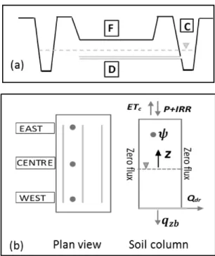
Figure 1a illustrates the cross section of a typical cranberry field while Figure 1b displays the plan view of the field along with the representation of a modelled soil column with boundary conditions. This simplified model concerns specifically the cranberry field which represents the heart of most activities occurring at a production site. During the growing season, the water level in the peripheral channel is kept constant. But even by doing so, the WTD below the cranberry
field is subjected to significant fluctuation owing to losses and hydrological processes; consequently the RMAP is also impacted. However, observations from different points shows that the WTD fluctuates slightly from one point to another and that an average WTD can be used without making significant error.
2.1 Formulation
The cranberry field is modelled as a soil column confined between the soil surface and the depth of the drainage-subirrigation system within which lays a water table (Figure 1). The flow of water in such medium is expressed as a coupled, saturated-unsaturated and vertical-horizontal flow equation (Equation 1). The first term on the right hand side of this equation corresponds to the original 1-D Richards (1931) equation; with 𝜓 [𝑘𝑃𝑎] being the soil matric potential, 𝐾 [𝑐𝑚/𝑑 ] the soil hydraulic conductivity and 𝑧 [𝑐𝑚] taken positive upward from the WTD. The drainage term (𝑄𝑑𝑟) is a sink term.
(1)
∂(𝐹𝑆𝑇𝑂)
∂𝑡 =
∂
[
𝐾(𝜓)(
∂𝜓∂𝑧+ 1)
]
∂𝑧 ‒ 𝑄𝑑𝑟
However, here we do not attempt to either numerically nor analytically solve Equation (1), but rather propose a computational approach to assess the water table depth and the root soil matric potential by representing the soil moisture and hydraulic conductivity profiles using well known functions through the steps that we describe hereinafter. We assume a static distribution of the soil matric potential in the unsaturated soil from which we derive the soil moisture and hydraulic conductivity profiles. The water budget of the soil column is then computed based on the concept of a control volume for which inflows minus outflows are balanced with the variation in storage on a daily time step (Equation 2). The daily time step is chosen because water requirements at a farm site are managed on a daily basis.
(2)
𝑑(𝐹𝑆𝑇𝑂)
Where, 𝑑(𝐹𝑆𝑇𝑂) is the field storage variation during time step , P, IRR, 𝑑𝑡 𝐸𝑇𝑐, 𝑞𝑧𝑏 and 𝑄𝑑𝑟 are respectively precipitation, irrigation, cranberry evapotranspiration, deep percolation and drainage rate; all occurring during a time step. Equation 2 is subjected to the boundary conditions shown in Figure 1b and thoroughly described under section 2.8 hereinafter.
Figure 1. Schematic of a typical cranberry field: (a): Cranberry field cross-section and major components : F=cranberry field, C=channel reservoir, D=drainage pipe; (b) plan view along with monitoring sites (grey spots) and boundary fluxes (arrows) of corresponding soil column. 𝑬𝑻𝒄: cranberry evapotranspiration, P: precipitation, IRR: irrigation, : soil matric potential, 𝝍 𝒒𝒛𝒃: deep percolation, 𝑸𝒅𝒓: drainage rate, : vertical axis taken positive upward from the water table 𝒁 depth (WTD).
2.2 Soil water retention functions (SWRFs)
The soil moisture content can be represented by the corresponding matric potential by means of either the Brooks et al. (1964) (BC) or the van Genuchten (1980) (VG) equations which are two widely-used models. They are presented in Equations (3) and (4), respectively.
𝑆𝑒=
{
𝜃 ‒ 𝜃𝑟 𝜃𝑠‒ 𝜃𝑟=(
ℎ𝑎ℎ)
𝜆𝐵𝐶 ℎ < ℎ𝑎 (3.𝑎) 1 ℎ ≥ ℎ𝑎 (3.𝑏)with 𝑆𝑒 [𝑐𝑚3/𝑐𝑚3] is the effective saturation, 𝜃 [𝑐𝑚3/𝑐𝑚3] the soil moisture, 𝜃𝑟 [𝑐𝑚3/𝑐𝑚3] and are respectively the residual and saturated soil moisture contents; is the
𝜃𝑠 [𝑐𝑚3/𝑐𝑚3] ℎ [𝑐𝑚]
pressure head; ℎ𝑎 [𝑐𝑚] the height of the capillary fringe (or the air entry pressure head in kPa) and 𝜆𝐵𝐶 [ ‒ ] the slope of the water retention curve. The last two parameters are governed by the pore size distribution curve of the studied soil.
𝑆𝑒=
{
𝜃 ‒ 𝜃𝑟 𝜃𝑠‒ 𝜃𝑟= 1[
1 +(
𝛼𝑉𝐺 ℎ)
𝑛𝑉𝐺]
1 ‒ 1 𝑛𝑉𝐺 ℎ < 0 (4.𝑎) 1 ℎ ≥ 0 (4.𝑏)With 𝛼𝑉𝐺 shifting the van Genuchten (VG) soil moisture left or right and 𝑛𝑉𝐺 being the slope of the curve. The soil matric potential [kPa] is one tenth of the total gravitational head.
2.3 Soil hydraulic conductivity and capillary length
The hydraulic conductivity profile of the unsaturated zone can be obtained either by the equation of Mualem (1976) (Equation 5) coupled with the van Genuchten model (VG-M) or by the Brooks and Corey (BC) hydraulic conductivity equation (Equation 6) derived from Burdine (1953) pore size distribution model, or by means of the Gardner exponential hydraulic conductivity function (Equation 7); where 𝐾𝑟 [𝑐𝑚/𝑑] is the relative hydraulic conductivity and 𝛼𝐺 [𝑐𝑚‒ 1] is the Gardner soil parameter which depends on the soil pore size distribution. The Gardner soil parameter represents the rate of reduction in the soil hydraulic conductivity. The finer the soil, the higher is the capillary rise and the smaller the Gardner parameter.
(5) 𝐾
(
𝑆𝑒)
= 𝐾𝑠𝑆𝑒[
1 ‒ (1 ‒ 𝑆𝑒1/𝑚)𝑚]
2 With 𝑚 = 1 ‒ 1/𝑛𝑉𝐺, 𝑛𝑉𝐺> 1 (6) 𝐾(
𝑆𝑒)
= 𝐾𝑠𝑆3 + 2 𝜆𝐵𝐶 𝑒(7) 𝐾𝑟=𝐾(ℎ)𝐾
𝑠 =
{
exp
(
𝛼𝐺ℎ)
ℎ < 0 1 ℎ ≥ 0ElsewhereFor,for the unsaturated soil constricted between the water table depth and the soil
surface, the ‘mean’ height of capillary rise above the water table, 𝐿𝑐𝑎𝑝 [cm] is assessed by means of Equation (8) (White et al. 1987) called the K-weighted mean soil water potential by Raats and Gardner (1971). As for the soil mean hydraulic conductivity, it is computed by Equation (9). the White et al. (1987) capillary length approach is used to assess the macroscopic capillary length, 𝐿𝑐𝑎𝑝 [cm] (Equation 8) as well as the mean unsaturated hydraulic conductivity (Equation 9). (8) 𝐿𝑐𝑎𝑝=
[
𝐾(
𝜓𝑠𝑢𝑝)
‒ 𝐾(
𝜓𝑖𝑛𝑓)
]
‒ 1∫𝜓𝑠𝑢𝑝 𝜓𝑖𝑛𝑓𝐾(𝜓)𝑑𝜓 (9) 𝐾(𝜓) = [𝜓𝑠𝑢𝑝‒ 𝜓𝑖𝑛𝑓 ]‒ 1∫𝜓𝑠𝑢𝑝 𝜓𝑖𝑛𝑓𝐾(𝜓)𝑑𝜓In the above equations, 𝜓𝑠𝑢𝑝 is the near saturation matric potential and 𝜓𝑖𝑛𝑓 [𝑘𝑃𝑎] is a more negative soil matric potential.
2.4 van Genuchten model capillary fringe and height
Using the van Genuchten model and assuming a hydrostatic condition, Shokri et al. (2011) derive for coarse textural soils, in which viscous forces are negligible, expressions to estimate the height of the capillary fringe ℎ𝑎_𝑉𝐺 (Equation 10) and the depth at which the water table cease to be hydraulically connected to the surface 𝐷𝑚𝑎𝑥 ; that is when the latter can no longer contribute efficiently to the soil evaporation (Equation 11). In case the soil hydraulic conductivity is represented by the Gardner expression, the inverse of the macroscopic capillary rise yields the Gardner parameter (Equation 12). 𝛼𝐺
(10.a) ℎ𝑎_𝑉𝐺=𝛼1 𝑉𝐺
[
(
𝑛𝑉𝐺 𝑛𝑉𝐺‒ 1)
2 ‒ 1/𝑛𝑉𝐺 ‒𝑛1 𝑉𝐺(1 + 𝑛𝑉𝐺 𝑛𝑉𝐺‒ 1) 2 ‒ 1/𝑛𝑉𝐺]
𝑛𝑉𝐺≥ 2 (10.b) ℎ𝑎_𝑉𝐺= 0 𝑛𝑉𝐺< 2(11) 𝐷𝑚𝑎𝑥=𝛼1 𝑉𝐺
[
1 ‒ 1 𝑛𝑉𝐺]
(1 ‒ 2𝑛𝑉𝐺) 𝑛𝑉𝐺 (12) 𝛼𝐺=𝐷1 𝑚𝑎𝑥2.5 Soil matric flux and matric potential
The soil matric potential gradient is controlled by the soil matric flux which under the assumption of an exponential hydraulic conductivity of the soil profile is written as follows (Yuan et al. (2005)
(see governing equations set out in the annexappendix).:
(13.a) 𝜓(𝑧) =𝛼1 𝐺𝑙𝑛
(
𝛼𝐺 𝛷(𝑧) 𝐾𝑠)
Where 𝛷(𝑧) =𝐾𝑠exp𝛼(‒ 𝛼𝐺𝑧) 𝐺 + 𝑞𝑧𝑠[exp(‒ 𝛼𝐺𝑧)‒ 1] 𝛼𝐺 + 𝑆0[(𝛼𝐺𝑧𝑠 + 1)exp(‒ 𝛼𝐺𝑧)‒ 𝛼𝐺(𝑧𝑠 ‒ 𝑧) ‒ 1] 𝛼𝐺2 (13.b) With 𝐾𝑠 [𝑐𝑚/𝑑] the saturated hydraulic conductivity, 𝑧𝑠 [𝑐𝑚] the distance to the soil surface from the WTD, 𝑞𝑧𝑠 [𝑐𝑚/𝑑] the infiltration, and 𝑆0 [𝑐𝑚/𝑑] the root uptake (evapotranspiration).For the case of no infiltration and no root uptake, these Yuan equations (Equation 13) yield a static pressure head. During the growing season, WTD is kept within the depth which allows optimal cranberry evapotranspiration. Such a constraint implies a constant flux from the water table to fulfill the plant water requirement. Hence, this steady-state matric flux from the water table becomes a coherent assumption.
2.6 Cranberry evapotranspiration
As shown in the appendix, Dduring the growing season, cranberry evapotranspiration is estimated by applying a cultural coefficient Kc=0.5 to the reference evapotranspiration (Equation
14) computed using the standardized Penman-Monteith model (Jensen and Allen, 2016)
(Equation 16). Allen et al. (1998) formula (Equation 15) or Hargreaves equation can be used to
approximate such reference evapotranspiration. The root uptake from the soil column is assumed to be uniform. In those equations: , daily solar radiation (MJ/m𝑅 2/d); , mean daily air
𝑎 𝑇
temperature (oC); 𝑇 , maximum daily temperature (oC); , minimum daily temperature
𝑚𝑎𝑥 𝑇𝑚𝑖𝑛
(oC); , latent heat of vaporisation (MJ/Kg), 𝐿 = density of water (Mg/m3), net radiation at
𝑒 𝜑𝑤 𝑅𝑛,
the crop surface (MJ/m2/d); sensible heat (MJ/m𝐺, 2/d); , wind speed at 2m height (m/s); , 𝑢
2 𝑒𝑠
saturated vapour pressure (kPa); , actual vapour pressure (kPa); 𝑒𝑎 𝑒𝑠‒ 𝑒𝑎, saturation vapour pressure deficit (kPa); , slope of the vapour pressure (kPa/𝛥 oC); = psychrometric constant 𝛾
(kPa/oC). (14) 𝐸𝑇𝑐= 𝐾𝑐∗ 𝐸𝑇𝑜 (15) 𝐸𝑇𝑜= 0.0023𝜑𝑅𝑎 𝑤𝐿𝑒(𝑇 + 17.8) 𝑇𝑚𝑎𝑥 ‒ 𝑇𝑚𝑖𝑛 (16) 𝐸𝑇𝑜=0.408 ∆ (𝑅𝑛‒ 𝐺)+ 𝛾 900 𝑇 + 273𝑢2(𝑒𝑠‒ 𝑒𝑎) ∆ + 𝛾(1 + 0.34 𝑢2) 2.7 Drainage computation
Cranberry field drainage is required if the WTD is such that the RMAP might be up to or larger than -3 kPa. Drainage can be assessed by means of the Guyon (1972) model (see the appendix for a description of the governing equations).expressed by Equations (17) and (18).
(17) 𝑄𝑑𝑟(𝑡) = 𝑄0𝛾 ∗ 𝐺 2(𝜔,𝛾,𝑡) + 𝐺(𝜔,𝛾,𝑡) 𝛾 + 1 And 𝑦 (0,𝑡) = 𝑦(0,0) (18.a) 𝑒𝜔𝑡+ 𝛾(𝑒𝜔𝑡‒ 1)= 𝑦 (0,0)𝐺(𝜔,𝛾,𝑡) where 𝐺(𝜔,𝛾,𝑡) = 1 (18.b) 𝑒𝜔𝑡+ 𝛾(𝑒𝜔𝑡‒ 1)
(18.c) 𝜔 = 𝑁4 𝑑𝑟 𝐾2 𝜇𝑑𝑟 𝛿 𝐸𝑑𝑟2 (18.d) 𝛾 =12 𝐾𝐾𝑠 𝑧𝑏 𝑦 (0,0) 𝛿 and
= water table height above the drain and at half distance between drains at time t (m) 𝑦(0,𝑡)
= saturated hydraulic conductivity of the soil column (m/s) 𝐾𝑠
= bottom boundary hydraulic conductivity (m/s) 𝐾𝑧𝑏
= - = drainage porosity (cm3/cm3)
𝜇𝑑𝑟 𝜃𝑠 𝜃𝑓𝑐
= distance between drains (m) 𝐸𝑑𝑟
= dimensionless variable 𝜔
δ = equivalent drainage depth (m);
and dimensionless coefficients depending on the shape of the water table;
𝑁𝑑𝑟 𝑃𝑑𝑟
= initial drainage rate (m3/s);
𝑄0
= drainage rate with respect to y(0,t) (m3/ s).
𝑄𝑑𝑟(𝑡)
2.8 Boundary conditions
Alike many hydrological models, the upper boundary is governed by atmospheric conditions which determine the daily surface fluxes (Equation 139). As shown in Figure 1a, the configuration of a cranberry field allows for total infiltration of the water reaching the ground, hence runoff and ponding are assumed negligible. Beside atmospheric conditions, the upper boundary is recurrently subjected to sprinkler irrigation to supplement any water deficiency in the root zone. Elsewhere, an irrigation efficiency coefficient may be useful to account for direct evaporation and any other losses which may occur through the irrigation system and for lack of uniformity of the irrigation (Irmak et al. 2011). This coefficient is useful if one has to derive the volume of water
from the duration of the irrigation. In case the field is equipped with a rain gage, the irrigation efficiency coefficient is simply set to unity. Equation (19) depicts the upper boundary condition:
(139) 𝑞𝑧𝑠= 𝑃 + 𝐼𝑅𝑅 ∗ 𝜂𝑖𝑟𝑟‒ 𝐸𝑇𝑐
As for the deep percolation or vertical/natural drainage, similar to the horizontal subsurface
drainage, it occurs only in the gravitational water and as in many land models (Dickinson et al. 1993, Mitchell et al. 2004, Oleson et al. 2004, Sellers et al. 1996), the flux to the deep ground water (percolation) is controlled by the saturated hydraulic conductivity of the soil lower frontier (Equation 2014). Elsewhere, the soil column lateral frontiers are subjected to zero flux boundary condition.
(2014) 𝑞𝑧𝑏= 𝐾(𝑧𝑏)
2.9 Computational steps
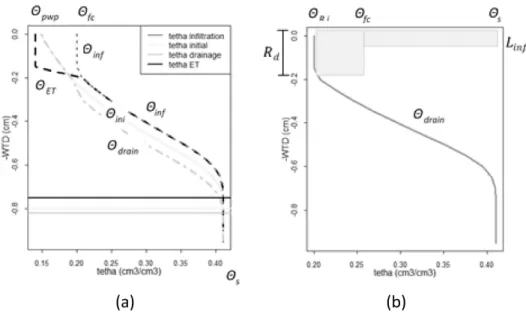
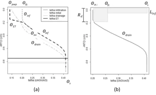
The model is based on the water budget of a uniform soil column discretized into several storage volumes (1, …, i-1, i, i+1,…,N numbered from top to the bottom of the soil column), being the 𝛥𝑧 size of each elementary volume. Regarding the WTD, the problem is solved considering steady state conditions while the RMAP is calculated in a transient state conditions. The steady state condition assumes that for a specific water table depth the soil matric flux reaches an equilibrium state where any further upward flux results in a drop in the water table. In such equilibrium state which assumes no infiltration into and no root uptake from the soil profile, the unsaturated soil moisture distribution is portrayed by the soil characteristic curve obtained from a static pressure head distribution; that is 𝜃𝑖𝑛𝑖 or in Figure 2.a. The transient state conditions take into 𝜃0 consideration the duration of the moisture wave diffusion through the root soil during infiltration to evaluate the daily RMAP. The hydrologic processes impacting the WTD (initially WTD0), the
RMAP and the soil water storage (FSTO, initially FSTO0) are computed in three major
(i) The first step is the computation of the soil drainage, that is, the percolation to the ground water and through the drainage system. The flux escaping the soil lower boundary is evaluated by means of the Darcy-Buckingham equation based on the initial WTD (WTD0) while the
horizontal subsurface drainage is calculated by means of the Guyon model. The total drainage
Wdr is deducted from the available gravitational water while preserving the soil water retention
gradient. The outcomes of this process are the soil moisture content 𝜃𝑑𝑟 and a deeper WTD (WTDdr) (Figure 2.a).
Figure 2. (a)Water table depth (WTD) and (b) root soil matric potential (RMAP) computational steps. 𝜽𝒑𝒘𝒑: soil moisture at wilting point, 𝜽𝒇𝒄: soil moisture at field capacity, 𝜽𝒊𝒏𝒇: soil moisture after infiltration, 𝜽𝑬𝑻: soil moisture after evapotranspiration, 𝜽𝒊𝒏𝒊: initial soil moisture , 𝜽𝒅𝒓𝒂𝒊𝒏: soil moisture content after drainage, 𝜽𝑹𝒊: initial mean root soil moisture, : saturated soil moisture 𝜽𝒔
content, : rooting depth, 𝑹𝒅 𝑳𝒊𝒏𝒇: length of the infiltration wave travelling through the root zone.
The following equations (Equations 21 15 to 2519) are solved to minimize the error ΔW𝑑𝑟 (see Equation 25). k is the number of discretized elementary volume affected by the drawdown; once
k is known WTDdr can be easily extracted. Δz [mm] is the discretization size and 𝜃𝑓𝑐 the soil
moisture at field capacity. The finer the discretization of the soil column, the more accurate is the result.
(215) 𝑊𝑇𝐷𝑑𝑟= 𝑊𝑇𝐷0+ 𝑘Δz
(1622.a) 𝜓𝑖= 𝑚𝑖𝑛
(
0, ‒ 𝑧𝑖)
𝑖 = 1,…, 𝑁Where is the position of th i𝑧 th elementary volume with respect to the WTD (Equation 22.b) 𝑖
(1622.b) 𝑧𝑖=‒ (𝑊𝑇𝐷0‒ (𝑖 ‒ 0.5)Δz)
Each elementary volume soil moisture content can be obtained by the following conditions depending on which SWRF is used:
if BC SWRF is used then each elementary storage moisture content is evaluated using Equation (2317): (1723.a) 𝜃𝑑𝑟(𝑖) =𝜃𝑖= 𝜃0(𝑖) 𝑖𝑓 𝜃0(𝑖) ≤ 𝜃𝑓𝑐 (1723.b)
{
𝜃𝑑𝑟(𝑖) =𝜃𝑖= max(
𝜃𝑓𝑐, 𝜃𝑟+(
𝜃𝑠‒ 𝜃𝑟)
( 𝜓𝑎 𝜓𝑖) 𝜆𝐵𝐶)
, 𝜓𝑖< 0 𝜃𝑑𝑟(𝑖) =𝜃𝑖= 𝜃𝑠, 𝜓𝑖≥ 0 If VG SWRF is used then each elementary storage moisture content is evaluated by means of Equation (23’17’): (1723’.a) 𝜃𝑑𝑟(𝑖) =𝜃𝑖= 𝜃0(𝑖) 𝑖𝑓 𝜃0(𝑖) ≤ 𝜃𝑓𝑐 (1723’.b)
{
𝜃𝑑𝑟(𝑖) =𝜃𝑖= max(
𝜃𝑓𝑐, 𝜃𝑟+ 𝜃𝑠‒ 𝜃𝑟[
1 +(𝛼𝑉𝐺𝜓𝑖)𝑛𝑉𝐺]
1 ‒ 1 𝑛𝑉𝐺)
, 𝜓𝑖< 0 𝜃𝑑𝑟(𝑖) =𝜃𝑖= 𝜃𝑠, 𝜓𝑖≥ 0The volume of water effectively drained from the soil column is evaluated by Equation (2418): (2418) W𝑑𝑟, 𝑒𝑓𝑓= ∑𝑁𝑖 = 1(𝜃0(𝑖) ‒𝜃𝑑𝑟(𝑖))Δz
And the minimized error is given by Equation (2519):
(2519) ΔW𝑑𝑟= W𝑑𝑟‒ W𝑑𝑟,𝑒𝑓𝑓
(ii) The second step requires the computation of the infiltration rate into the soil profile. It is noteworthy the configuration of cranberry fields, protected by embankments, allows total infiltration of the water reaching the ground, that is the cumulated precipitation and irrigation (Equation 19), hence runoff, is negligible. Infiltration impacts significantly the WTD and the RMAP. Infiltration into the soil profile is computed in two stages which are meant to fulfill the field capacity and soil saturation requirements. Up to the field capacity level, water is held in the soil column from top to bottom and beyond the field capacity the excess water diffuses through the soil column down to the water table.
With regard to the WTD, during the first stage, that of field capacity requirement, water is distributed from top to bottom across discretized storage volumes while limiting each storage soil moisture content to the field capacity level as in Equations (206) to (30) and (23) where 𝜃𝑖𝑛𝑓,1
[cm3/cm3] and [cm3/cm3] correspond to the moisture content of ith storage volume after
(𝑖) 𝜃𝑖,1
the drainage and first infiltration stages, respectively, 𝑞 [mm] is the inflow of water in the ith 𝑖 ‒ 1
storage volume or the outflow volume from the i-1th storage volume.
(206) 𝑞0= 𝑞𝑧𝑠
For the ith discretized storage volume, the volume of water needed to fulfill the field capacity
level is assessed by Equation (217):
(217) ∆𝑉𝑓𝑐(𝑖) = max (0, (𝜃𝑓𝑐‒ 𝜃𝑑𝑟(𝑖)))∆𝑧
From top to bottom, the volume of water stored in the ith elementary volume during this first
stage of the infiltration, is evaluated by Equation (228) and the remainder of the infiltration volume of water reaching the i+1th storage is giving by Equation (239). At the end of this first
stage of the infiltration, each discretized soil water content is assesd by Equation (3024) and the total volume of water distributed during this first infiltration stage is calculated using Equation (3125). (228) 𝑊𝑓𝑐(𝑖) = min (𝑞𝑖 ‒ 1, ∆𝑉𝑓𝑐(𝑖)) (239) 𝑞𝑖= max (0, (𝑞𝑖 ‒ 1‒ ∆𝑉𝑓𝑐(𝑖)) (2430) 𝜃𝑖𝑛𝑓,1(𝑖) = min
(
𝜃𝑑𝑟(𝑖) + 𝑊∆𝑧𝑓𝑐(𝑖), 𝜃𝑓𝑐)
(2531) 𝑊𝑖𝑛𝑓1 = ∑𝑁𝑖 = 1(𝜃𝑖𝑛𝑓,1(𝑖) ‒ 𝜃𝑑𝑟(𝑖))The second stage of the infiltration inherits the remainder of the infiltration after completeness of the first infiltration stage, that is . As during the drainage process, the number of discretized 𝑞𝑁
storage volume affected by the rising of the water table, that is k’ (Equation 3226) is searched. At this point the model seeks for a new WTD by preserving the slope of the SWRF, that is, we assume that the soil moisture profile at the end of this process has reached a steady state described by a linear distribution of the soil matric potential (Equation 3327). is distributed 𝑞𝑁 across the SWRF to find the likely WTD (WTDinf) from which the soil moisture profile 𝜃𝑖𝑛𝑓 is
obtained. In doing so, each elementary soil volume moisture content is obtained using either the BC SWRF (Equation 3428) or VG SWRF (Equation 2834’). The effectively distributed volume of water W𝑖𝑛𝑓,𝑒𝑓𝑓 is evaluated by Equation (3529) and the minimized error ΔW𝑖𝑛𝑓 is calculated by Equation (306). The prevailing soil moisture profile at the end of the infiltration is shown in Figure (2.a) from which the root soil mean moisture (RSMO) at the end of the infiltration, that is 𝜃𝑓,𝑊𝑇𝐷 is derived. (326) 𝑊𝑇𝐷𝑖𝑛𝑓= 𝑊𝑇𝐷𝑑𝑟‒ 𝑘'Δz (2733.a) 𝜓𝑖= 𝑚𝑖𝑛
(
0, ‒ 𝑧𝑖)
𝑖 = 1,…, 𝑁 (2733.b) 𝑧𝑖=‒ (𝑊𝑇𝐷𝑑𝑟‒ (𝑖 ‒ 0.5)Δz) if BC SWRF is used then each elementary storage moisture content is evaluated using: (3428)
{
𝜃𝑖𝑛𝑓(𝑖) =𝜃𝑖= max(
𝜃𝑖𝑛𝑓,1, 𝜃𝑟+(
𝜃𝑠‒ 𝜃𝑟)
( 𝜓𝑎 𝜓𝑖) 𝜆𝐵𝐶)
, 𝜓𝑖< 0 𝜃𝑖𝑛𝑓(𝑖) =𝜃𝑖= 𝜃𝑠, 𝜓𝑖≥ 0 If VG SWRF is used then each elementary storage moisture content is evaluated using:
(2834’)
{
𝜃𝑖𝑛𝑓(𝑖) =𝜃𝑖= max(
𝜃𝑖𝑛𝑓,1, 𝜃𝑟+ 𝜃𝑠‒ 𝜃𝑟[
1 +(𝛼𝑉𝐺𝜓𝑖)𝑛𝑉𝐺]
1 ‒ 1 𝑛𝑉𝐺)
, 𝜓𝑖< 0 𝜃𝑖𝑛𝑓(𝑖) =𝜃𝑖= 𝜃𝑠, 𝜓𝑖≥ 0 (3529) W𝑖𝑛𝑓,𝑒𝑓𝑓= ∑𝑁𝑖 = 1(𝜃𝑖𝑛𝑓(𝑖) ‒𝜃𝑑𝑟(𝑖))Δz (306) ΔW𝑖𝑛𝑓= W𝑖𝑛𝑓‒ W𝑖𝑛𝑓,𝑒𝑓𝑓The daily RMAP is the result of a dual effect of the static pressure head due to the presence of the shallow WTD and that of the infiltration. It is computed (Equation 317) using the concept of infiltration wave diffusion time through the soil column (Equation 328). During infiltration, the wetting front propagates through the soil and the mean RMAP may go through three stages: rising, constant, or falling RMAP or root soil moisture (RSMO). The rising stage corresponds to the accumulation of moisture within the root zone until a maximum mean RSMO is reached. Such maximum lasts in the root zone for a period of time and then gives way to a falling RSMO branch which sets up either when the wetting front starts to percolate out of the root zone, if the maximum mean RSMO is less than the saturation moisture content, or at the moment infiltration has ended if the maximum mean RSMO is equivalent to the saturated moisture content.
(317) 𝑅𝑀𝐴𝑃 = (𝜓𝑊𝑇𝐷Δ𝑡𝑊𝑇𝐷+ 𝜓𝑖𝑛𝑓𝛥𝑡𝑖𝑛𝑓)/𝑡𝑑𝑎𝑦
where:
is the mean RMAP due to the presence of the shallow water table (kPa); 𝜓𝑊𝑇𝐷
is the mean RMAP prevailing in the root zone during infiltration (kPa); 𝜓𝑖𝑛𝑓
and are durations of and of , respectively (hr);
Δ𝑡𝑊𝑇𝐷 Δ𝑡𝑖𝑛𝑓 𝜓𝑊𝑇𝐷 𝜓𝑖𝑛𝑓
the time step (day that is 24hr). 𝑡𝑑𝑎𝑦
(328) 𝑅𝑀𝐴𝑃 =[𝜓0Δ𝑡1+ 𝜓𝑓𝑐𝛥𝑡2+ 𝜓𝑡 𝑚𝑎𝑥𝛥𝑡3 + 𝜓𝑓Δ𝑡𝑓]
𝑑𝑎𝑦
Where
is the mean RMAP due to the root soil initial moisture content (kPa); 𝜓0
is the field capacity RMAP (kPa); 𝜓𝑓𝑐
is the root zone maximum mean RMAP equivalent to the maximum RSMO (kPa); 𝜓𝑚𝑎𝑥
is the final mean RMAP with respect to the final root soil moisture (kPa);
𝜓𝑓 𝜃𝑓
duration of the initial RSMO (hr); 𝛥𝑡1= 𝑡(𝜃𝑅𝑖)
duration of RSMO field capacity (hr); 𝛥𝑡2= 𝑡
(
𝜃𝑓𝑐)
duration of during constant RSMO stage (hr); 𝛥𝑡3= 𝑡
(
𝜃𝑅𝑚𝑎𝑥)
𝜓𝑚𝑎𝑥duration of equivalent to the final RSMO over the day (hr); 𝛥𝑡𝑓= 𝑡
(
𝜃𝑓)
𝜓𝑓An optimal discretisation of the daily time is necessary to obtain reliable results. The finer the time discretisation the more accurate the result. While a coarse discritisation may not give sufficient data to obtain a satisfactory result, a cumbersomely finer discritisation may be just useless by not being able to improve significantly the result. We adopt an hourly discretisation of the day time to obtain a satisfactory outcome. The infiltration rate at time t is controlled by the
total volume of precipitation and irrigation (𝑄𝑧𝑠𝑡) and the root zone mean hydraulic conductivity at that time (Equation 339). The subsequent RSMO (𝜃𝑡 + 1𝑅 ) is evaluated from Equation (34)0.
(339) 𝑞𝑅𝑡 = min (𝑞𝑧𝑠𝑡,𝐾(𝜃𝑅𝑡))
(340) 𝜃𝑡 + 1𝑅 = 𝜃𝑅𝑡 + 𝑞𝑅𝑡/𝑅𝑑
The soil moisture wave diffusion through the root zone occurs only if the maximum mean RSMO (𝜃𝑅𝑚𝑎𝑥) caused by the infiltration (Equation 4135) is beyond the field capacity level and merely the surplus moisture to the field capacity level will percolate through the root zone. The depth of the wetting front equivalent to that surplus of water (Equation 42 36 and Figure 2.b) travels across the root zone at the rate of the soil saturated hydraulic conductivity over a distance 𝐷𝑝 (Equation 437) during 𝛥𝑡3 over which the maximum mean RMAP/RSMO will prevail in the root zone. In these equations, 𝜃 initial mean root soil moisture (cm3/cm3); rooting depth (mm);
𝑅,𝑖, 𝑅𝑑,
total infiltration volume (mm); length of the infiltration wave travelling through the root
𝑞𝑧𝑠, 𝐿𝑖𝑛𝑓, zone (mm). (4135) 𝜃𝑅𝑚𝑎𝑥= min (𝜃𝑅,𝑖+𝑞𝑅𝑧𝑠 𝑑,𝜃𝑠) (4236) 𝐿𝑖𝑛𝑓= 𝑅𝑑
[
𝜃𝑅𝑚𝑎𝑥‒ max(
𝜃𝑅,𝑖,𝜃𝑓𝑐)
]
/[𝜃𝑠‒ max(𝜃𝑅,𝑖,𝜃𝑓𝑐)] (4337) 𝐷𝑝= max(
0,𝑅𝑑‒ 𝐿𝑖𝑛𝑓)
When infiltration is completed and the moisture front is percolating out of the root zone, the RMAP starts to degrade until the final root soil moisture (Equation 𝜃𝑓 4438). The destiny of the total volume of water which percolates out of the root zone contributes to the rise of the water table at the end of the day, hence impacting the daily final RMAP/RSMO, that is or 𝜓𝑓 𝜃𝑓,𝑊𝑇𝐷 (see WTD computational steps). If the final RSMO is less than or equal to the field capacity level, its equivalent RMAP will last until the end of the day and the durations 𝛥𝑡2 and 𝛥𝑡𝑓 are simply nil; while in the reverse case where the final RSMO is greater than the field capacity level, the RMAP of that RSMO will last the rest of the day.
(3844.a) 𝜃𝑓= 𝜃𝑅𝑚𝑎𝑥 , 𝜃𝑅𝑚𝑎𝑥≤ 𝜃𝑓𝑐
(3844.b) 𝜃𝑓= max
(
𝜃𝑓,𝑊𝑇𝐷, 𝜃𝑓𝑐)
, 𝜃𝑅𝑚𝑎𝑥> 𝜃𝑓𝑐The third and final step is the computation of the soil evaporation or root water uptake which is deducted from the water table if the latter is within the depth at which the ground water is hydraulically connected to the surface; otherwise a uniform root uptake is deducted within the root zone until the daily evaporation demand is fulfilled. The deduction of evapotranspiration from the water table results in a drop of the WTD and a shift to the left hand side of the SWRF while in the second case scenario the root soil dry out with respect to the plant permanent wilting point. This final process leads to the ultimate WTD which is recorded at the end of the day. The available moisture for evaporation in the ith volume storage is evaluated as in Equation (4539)
and the remainder of the evaporation needs is assessed by Equation (406). This is done for several control volumes if necessary so as to minimize the error (𝐸𝑇𝑟𝑒𝑠) associated to this process. At the end of this process, the soil profile field storage (FSTO) can then be computed using Equation (417) and the daily residue of the water balance using Equation (428). For a simulation over Nd,
number of days, the biais is evaluated as the sum of the daily residues over the period of the simulation (Equation 439). (4539) 𝐸𝑇𝑖, 𝑎𝑣= max
(
0, 𝜃𝑖‒ 𝜃𝑚𝑖𝑛, 𝐸𝑇)
∗ ∆𝑧 (406) 𝐸𝑇𝑟𝑒𝑠= max (0, 𝐸𝑇𝑐‒ 𝐸𝑇𝑖, 𝑎𝑣) (417) 𝐹𝑆𝑇𝑂 = ∑𝑁𝑖 = 1𝜃(𝑖) (428) 𝑊𝐵𝑅 = ∆𝑊𝑑𝑟+ ∆𝑊𝑖𝑛𝑓+ 𝐸𝑇𝑟𝑒𝑠 (439) 𝛥𝛥 = ∑𝑁𝑑 𝑗 = 1𝑊𝐵𝑅(𝑗) Where := the available volume of water for evaporation in the ith control volume (mm);
= cranberry permanent wilting point (mm); 𝜃𝑚𝑖𝑛, 𝐸𝑇
= daily water budget residue (mm) ; 𝑊𝐵𝑅
= biais of a simulation over Nd number of days (mm).
𝛥𝛥
3 SITE INSTRUMENTATION AND FIELD MONITORING
For this study, a cranberry field site was instrumented to validate the model. Field equipment included a weather station to collect the required information for the computation of the standardized Penman-Monteith evapotranspiration and to monitor the soil matric potential and the WTD. The RMAP was monitored at a depth of 20 cm, that is, just below the root zone (see Figure 1b). The grey dark circles on Figure 1b represent the locations of the tensiometers and the grey lines the locations of the drains. The investigation was carried out at a site located (46.30 N, 71.88 W and 111m altitude) in Quebec, Canada. The site under investigation has a surface area of 10.5 hectares. The site soil physical characteristics are summarized in Table 1.
4 RESULTS AND DISCUSSION
4.1 Model parameterization
The van Genuchten parameters of the soil samples were determined by fitting experimental drying and wetting suction head laboratory test results to the model using Hydrus 1D (Simunek et al. 2005). The average of the drying and wetting mean values (𝑁𝑉𝐺 and 𝛼𝑉𝐺) were used to represent the soil VG parameters as no hysteresis was accounted for. The maximum depth at which the water table is no longer hydraulically connected to the soil surface (Dmax), the Gardner
hydraulic conductivity parameter ( ) and the air-entry pressure head (hαG a) were then
approximated from those median VG parameters value by means of analytical expressions introduced by Shokri et al. (2011). The result of such approximation were 13.3 cm, 0.74, and 9.63 cm for Dmax, , and hαG a, respectively; the VG median parameters, representing the diversity
the BC parameters were derived by preserving the soil macroscopic capillary length (Lcap) under
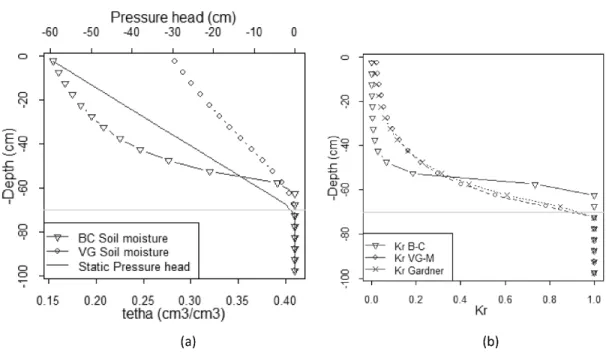
the assumption of a hydrostatic pressure head distribution bounded by a zero matric potential (at the WTD) and a minimum allowable RMAP of -7.5 kPa. Figures 3a and 3b show the soil moisture and hydraulic conductivity patterns for the two models (VG-M and BC).
Table 1. Site soil parameters. 𝑵𝑽𝑮: drying mean value, 𝜶𝑽𝑮: wetting mean value, Dmax : maximum depth at which
the water table is no longer hydraulically connected to the soil surface, Lcap : soil macroscopic
capillary length, 𝑲𝑽𝑮: mean hydraulic conductivity for van Genuchten model, Ksat :saturated
hydraulic conductivity, ha : air-entry pressure head, λBC : slope of the water retention curve,
: mean hydraulic conductivity for Brooks and Corey model, : Gardner hydraulic
𝑲𝑩𝑪 𝛂𝐆
conductivity parameter, 𝑲𝑮: mean hydraulic conductivity for Gardner model.
van Genuchten Brooks and Corey Gardner
NVG [-] αVG [cm] 𝐷𝑚𝑎𝑥 [cm] [cm]Lcap /Ksat 𝐾𝑉𝐺 [-] ha [cm] λ[-]BC [cm]Lcap /Ksat 𝐾𝐵𝐶 [-] 𝛼𝐺 [cm-1] Lcap [cm] /Ksat 𝐾𝐺 [-] 1.832 0.236 80.6 15.4 0.22 10.2 0.7 14.0 0.21 0.075 13.8 0.20
Figure 3. Unsaturated soil moisture and hydraulic conductivity: (a) Soil moisture curves, (b) Relative hydraulic conductivity curves. theta: soil moisture, h: soil pressure head (cm), Kr: relative hydraulic conductivity, VG-M: van Genuchten Mualem model, BC: Brooks and Corey model.
4.2 Model theoretical and experimental validations
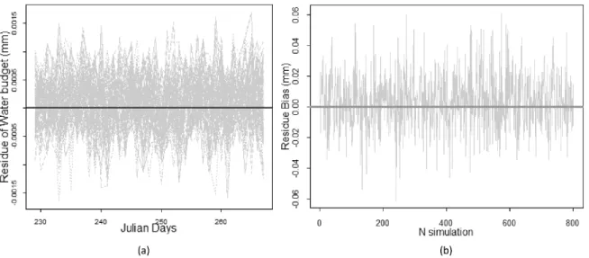
The model was validated theoretically and experimentally. The theoretical validation pertained to the water budget, while the experimental validation was carried out with respect to observed values of WTD and RMAP. Figure 4 introduces the daily residues of the water balance calculated over 800 model simulations. The values fluctuate slightly around zero while the daily bias is always below ± 0.06 mm and deemed negligible.
The experimental validation was carried out with respect to observed values of WTD and RMAP. Recorded site data belonged to the west and center site monitoring points displayed in Figure 1a. Note that the eastern monitoring point apparatus was faulty. To determine the prevailing and likely lower boundary condition, deep percolation fluxes were analysed for days without recorded precipitation or irrigation. The results indicated that the lower boundary flux ranged from -2.0 to 0.5 cm/day and is 90% of the time negative. This means that the soil profile is under drainage conditions as the fluxes represent water exiting the soil column (i.e., deep percolation). The positive fluxes are the resulting effects of the subirrigation which outweighed the deep percolation during very few days only, exhibiting a lack of efficiency of the subirrigation system. This prevailing condition justifies the needs of sprinkler irrigation to satisfy plant daily water requirements.
Figure 4. Theoretical validation of the soil water balance over 800 computational experiments: (a) daily residues and (b) daily bias.
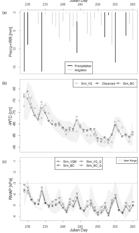
Regarding WTD (Figures 5b), the daily range (minimum and maximum values of continuously recorded data) is displayed with a grey shaded area, the daily mean value of the two monitoring sites (see Figure 1b) is shown by a hollow triangle oriented upward and the results of the simulations are exhibited by dashed lines with hollow circles for the VG SWRF and with hollow triangles oriented downward for the BC SWRF. As for the RMAP, the observed mean values for the two monitoring sites are displayed in grey while the results of the simulations are unveiled in dashed lines and various circles: hollow circles (respectively hollow squares) for the VG-M model (respectively VG_G, VG with Gardner hydraulic conductivity), and hollow triangles oriented downward (respectively the x) for the BC model (respectively BC_G, BC with Gardner hydraulic function). Figure 5a represents daily precipitation and irrigation events over the experimental period. For most of the days, the water table decreases (except for significant rainfall events) confirming the earlier finding that the soil is under drainage conditions mostly. The ideal situation is to have the simulated values of WTD and RMAP between the daily ranges of WTD and the daily median range of RMAP. For both variables, the simulation and the data behave similarly and most of the time the results fit well into the prescribed range. However, the WTD displayed a certain delay in responding to a precipitation event. This is not surprising given the use of a static model. Elsewhere between the observed values (from the first observation position and the second observation position), the range of mean daily WTD variation is very little and, hence, represented in a single line while that of the RMAP displays a wider interval showing variation in the soil capillary ability. The simulations performed with VG coupled with Mualem (VGM) and Gardner hydraulic conductivity (VG_G) models predict similar RMAP values (Figure 5c, circles and crosses) because the parameterized Gardner hydraulic curve matches perfectly the VGM curve within the vadose zone (see Figure 3b). As for the BC hydraulic conductivity model the predicated RMAP (Figure 5c, hollow triangles) are slightly above the rest of the simulated values because of the sharp decrease and falling of the BC hydraulic conductivity which falls below the VGM and VG_G models (Figure 3b) hence causing the infiltration water to remain a longer time within the root soil.
Figure 5. Experimental validation of the model: (a) water inputs from precipitation (Precip) and irrigation (IRR), (b) water table depth (WTD), and (c) root soil matric potential (RMAP). VG: van Genuchten Mualem model, BC: Brooks and Corey, VGM: van Genuchten Mualem model coupled with Gualem hydraulic conductivity model, VG_G: van Genuchten Mualem model coupled with
Gardner hydraulic conductivity model. BC_G: Brooks and Corey coupled with Gardner hydraulic conductivity model.
The performance of the model was also quantitatively assessed using two metrics: a system of score for both WTD and RMAP; that is a score of 1 was attributed to the result if the simulated value was within the range of daily values for that day otherwise a score of zero was given and that performance was calculated as the ratio of the cumulative score over the length of the simulation period. In addition, the WTD performance was assessed using the Kling Gupta Efficiency (KGE) metric which can be decomposed into the Pearson correlation coefficient (r), the bias ratio defined by the ratio between the mean values ( ), and the variability ratio obtained by 𝛽 the ratio of the coefficients of variation (standard deviation over mean value, ) (Gupta et al. 𝛾 2009, Kling et al. 2012). KGE, r, , and are all dimensionless and are optimum at unity. 𝛽 𝛾
(1544.a) 𝐾𝐺𝐸 = 1 ‒ (𝑟 ‒ 1)2+ (𝛽 ‒ 1)2+ (𝛾 ‒ 1)2 (1544.b) 𝛽 =𝜇𝜇𝑠𝑖𝑚 𝑜𝑏𝑠 (1544.c) 𝛾 =𝐶𝑉𝐶𝑉𝑠𝑖𝑚 𝑜𝑏𝑠= 𝜎𝑠𝑖𝑚 𝜇𝑠𝑖𝑚 𝜎𝑜𝑏𝑠 𝜇𝑜𝑏𝑠
The results of the model performance with respect to each variable is presented in Table 2; the values in brackets represent the KGE components respectively r, , and . The median field 𝛽 𝛾 storage (FSTO) for the 800 experiments from Sobol method is evaluated at 338.07 mm for the BC model and 374.43mm for the VG model, which is logical as the VG soil water retention function (SWRF) curve is wetter than that of BC.
Table 2. Model performance for water table depth (WTD) and root soil matric potential (RMAP). The values in brackets represent the KGE components respectively r, , and . SWRF: soil water retention 𝜷 𝜸
function, KGE: Kling Gupta Efficiency metric, VGM: van Genuchten model, BC: Brooks and Corey model.
Performance RMAP (Score) [%] Performance WTD [%] Hydraulic conductivity models
van Genuchten SWRF 78.13 88.59 (0.89;1.00;0.99) 71.87 - 75.00 Brooks and Corey SWRF 78.13 86.93 (0.88;1.00;0.95) - 65.63 71.88
4.3 Sensitivity and uncertainty analysis
The sensitivity analysis of the model was conducted using the Morris (1991) global sensitivity screening method to sort out the most influential parameters on model output. Indeed, the Morris method generates less input data than other stochastic methods such as Monte Carlo and Sobol method, hence, is very efficient in term of computation time required to perform the global sensitivity analysis. The experiment starts by generating a set of new random values for each parameter within the range of possible values introduced in Table 3. Then, in a subsequent experiment, only a single parameter value is randomly generated while preserving the rest of the parameter values in the preceding experiment until all parameter values are changed. The experiment is repeated ten (10) times for eight parameters starting each time with a new set of parameter values (8 + 1) leading to ninety (90) experimentations.
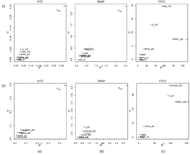
The intervals of Gardner parameter values were chosen from estimates given by Khaleel et al. (2001) for coarse texture soils, while the van Genuchten soil parameters were chosen from estimates by means of the Rosetta computer program (Schaap et al. 2001). For the rest of the parameters, the minimum and maximum values were taken from the Rawls et al. (1982) estimates for the Brooks and Corey water retention function for sandy soils. The results of the Morris experiment are shown in Figure 6, where μ* represents the sole influence of a parameter on the model output and σ characterises the interaction of a parameter with other parameters on the model output. The results indicate that WTD and RMAP are heavily impacted by the lower boundary condition 𝐾𝑧𝑏 for both SWRFs. The lower boundary condition interacts in order of importance with the slope of the water retention curve, the height of the capillary fringe, the soil saturated hydraulic conductivity, the saturation moisture content and, to a least extent, the field capacity and the residual moisture content; that is 𝑛𝑉𝐺, 𝛼𝑉𝐺, , 𝜃𝑠 𝜃𝑓𝑐, for the VGM model and 𝜃𝑟
, , , , for the BC model with regard to the WTD and , , , , , for the
ℎ𝑎 𝜆 𝜃𝑠 𝜃𝑓𝑐 𝜃𝑟 𝑛𝑉𝐺 𝛼𝑉𝐺 𝐾𝑠 𝜃𝑠 𝜃𝑓𝑐 𝜃𝑟
except parameters with less influential effects the rest has a non-linear effect with or without interaction with others. Elsewhere, the field storage (FSTO), the auxiliary variable of the model, is mostly and non-linearly affected by the slope of the water retention curve, the air-entry pressure head or the capillary length, the saturated and residual soil moisture, respectively. In using the model due attention should be given to parameters in the same order of importance as displayed by the sensitivity analysis result.
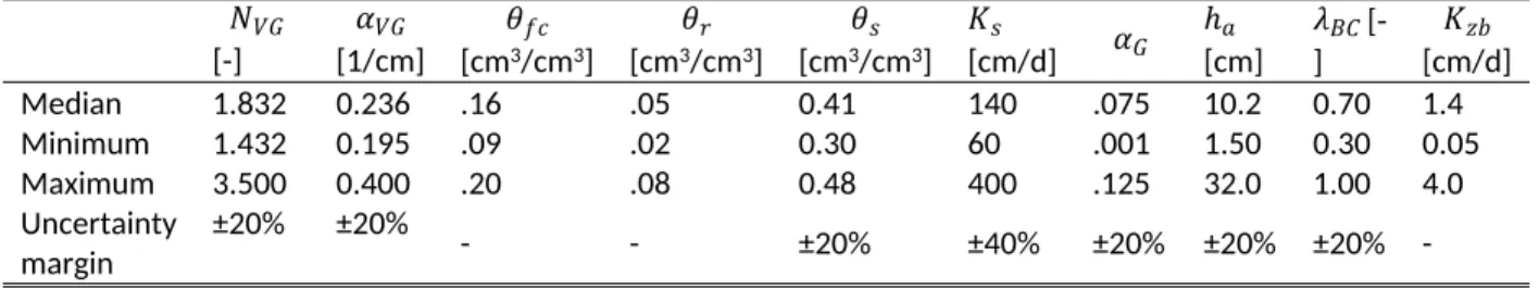
Table 3. Soil physical characteristics (median values, sensitivity range and uncertainty analysis margin). 𝑵𝑽𝑮: drying mean value, 𝜶𝑽𝑮: wetting mean value, 𝜽𝒇𝒄: soil moisture at field capacity, 𝜽𝒓: residual soil moisture content, : saturated soil moisture content, : saturated hydraulic conductivity, : 𝜽𝒔 𝑲𝒔 𝜶𝑮
Gardner hydraulic conductivity parameter, : air-entry pressure head,𝒉𝒂 𝝀𝑩𝑪: slope of the water retention curve, 𝑲𝒛𝒃: bottom boundary hydraulic conductivity.
𝑁𝑉𝐺 [-] 𝛼𝑉𝐺 [1/cm] 𝜃𝑓𝑐 [cm3/cm3] 𝜃𝑟 [cm3/cm3] 𝜃𝑠 [cm3/cm3] 𝐾𝑠 [cm/d] 𝛼𝐺 ℎ[cm]𝑎 𝜆]𝐵𝐶 [- [cm/d]𝐾𝑧𝑏 Median 1.832 0.236 .16 .05 0.41 140 .075 10.2 0.70 1.4 Minimum 1.432 0.195 .09 .02 0.30 60 .001 1.50 0.30 0.05 Maximum 3.500 0.400 .20 .08 0.48 400 .125 32.0 1.00 4.0 Uncertainty margin ±20% ±20% - - ±20% ±40% ±20% ±20% ±20%
-Figure 6. Sensitivity plots of the Morris method: (i) van Genuchten (VG) model, (ii) Brooks and Corey (BC) model; (a) water table depth (WTD), (b) root soil matric potential (RMAP) and (c) field storage (FSTO). N_VG: drying mean value, alfa_VG: wetting mean value, theta_cc : soil moisture at field capacity, theta_res: residual soil moisture content, theta_sat : saturated soil moisture content, Ksat: saturated hydraulic conductivity, alfa_G : Gardner hydraulic conductivity parameter, h_air: air-entry pressure head, lambda_BC: slope of the water retention curve, 𝑲𝒛𝒃: bottom boundary hydraulic conductivity.
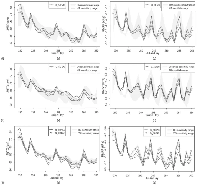
An uncertainty analysis was conducted to assess the influence of variations in the soil parameters on the model outputs. The use of Sobol (1993) method led to 800 experiments randomly selected from uniformly distributed input variables within the uncertainty margins introduced in Table 3. Those margins were apportioned based on deviations obtained from laboratory tests conducted on 20 soil samples taken from the site under investigation. The intervals are small due to fact that cranberry farm unlike other types of farms have man-made fields, constructed with mostly homogenous sandy soils. The WTD and RMAP uncertainty ranges are computed for ninety
percent confidence interval in continuous black lines and the median values are represented in discontinuous black lines and points (hollowed square points for the VG model, Figures 7.i and 7.iii and hollowed triangle points for the BC model, Figure 7.ii and 7.iii for the BC model). The grey shaded areas for the WTD (Figure 7.i.a and 7.ii.a) and the RMAP (Figures 7.i.b and 7.ii.b) representing respectively the daily minimum and maximum range of recorded site data compare them to the sensitivity variation range and mean value of the model output. The results show that both variables are similarly sensitive to parameter values (Figures 7.iii.a and 7.iii.b) but with variable magnitude (Figures 6.i.a vs Figure 6.ii.a and Figure 6.i.b vs Figure 6.ii.b).
Figure 7. Uncertainty analysis for: (i) van-Genuchten (VG) Model, (ii) Brooks and Corey (BC) Model, and (iii) comparison between VG and BC models, with respect to: (a) water table depth (WTD) and (b) root soil matric potential (RMAP).
As depicted in Figure 7, the median WTD and RMAP responses for both the van Genuchten and Brooks and Corey models are normally distributed as their respective median lays midway between their respective tenth and ninetienth percentile. The range of variation for both variables and for both models is less than the daily variation range of the observed data for the site, which highlights the robustness of the models. In addition, the sensitivity range variations of both models are similar.
5 CONCLUSION
The aim of this study was to develop a simplified water management mathematical tool capable of predicting the water table depth and the root soil matric potential of a cranberry field under a dual subirrigation-drainage system. The model was developed using the most widely used analytical soil water retention functions (SWRF), those of van Genuchten and Brooks and Corey coupled respectively with the Mualem and Brooks and Corey hydraulic conductivity functions while both SWRF can be used as well with the Gardner hydraulic conductivity function. Those functions were applied under a steady state framework to a uniform soil column which was discretized into finite soil storage volumes.. Both SWRFs reproduce the same mean WTD with about 75% success and were normally distributed when subjected to uncertainty analysis. As for the RMAP, better predictions are obtained with the Gardner hydraulic conductivity function and that of VG-M with the BC hydraulic conductivity giving the lowest success. The RMAP output is also normally distributed for the VG and BC models. The lower boundary condition of the model influences significantly the model outputs and due attention should be given to it. To ascertain the consistency and the reliability of the model, additional in-situ surveys will be carried out for other growing seasons for the site under investigation as well as for other sites. This model will pave the way to several other studies, for example studying: (i) the effect of the soil type on the cranberry plant annual water demand, (ii) the impact of small changes in the lower boundary condition on water demand, (iii) the impact of climate variability and climate change on the plant water demand.