En vue de l'obtention du
DE
DE T
Délivré par l'Université Toulouse III - Paul Sabatier Discipline ou spécialité : Océanographie Spatiale
Présentée et soutenue par Hindumathi Kulaiappan Palanisamy
Le 06 janvier 2016
Titre: Le niveau de la mer actuel: variations globale et régionales
Title: Present day sea level: global and regional variations
JURY
Nicholas Hall (Président du Jury) Jérôme Vialard (Rapporteur) Johnny A. Johannessen (Rapporteur)
Joshua Willis (Examinateur) Anny Cazenave (Directrice de Thèse) Thierry Delcroix (Directeur de Thèse)
Ecole doctorale: SDUEE
Unité de recherche: LEGOS UMR 5566
Directeurs de Thèse: Anny Cazenave et Thierry Delcroix Rapporteurs: voir le Jury
iii
Acknowledgements
I would first like to thank Anny for her marvelous support all through the duration of this thesis. Her vast knowledge is highly impressive and her curiosity to learn new things has always been a motivating factor to me. Through her, I learnt that neither age nor intellectual status is a barrier when it comes to constant quest for knowledge. I am also impressed with the importance she has given and still continues to give her students irrespective of her schedule. I am deeply honored to be one of her students.
I would also like to thank Thierry for his patience, pedagogic skills and his vast knowledge in the field of oceanography. His astonishing ability to explain concepts in a very simple manner has been of great help for someone like me having no prior education in the domain of oceanography. Our Thursday discussions have also helped me uncover his humorous and easy-going attitude!
I would also to acknowledge the financial support from CNES and CLS and thank Michaël, Gilles for their support in obtaining the financement.
My sincere thanks to Philippe; without his help I would not have been able to start my career in this field of research. I would also like to thank Benoit and Mélanie who have both been my first mentors. It’s still a great pleasure to discuss and learn a lot from you both.
My special thanks to Martine, Nadine, Catherine and Agathe for their help with the paper works irrespective of their workloads. I still remember the days when I hardly spoke French and would go to them for help. If not for them, I would have had a tough time getting adapted at LEGOS.
Thanks to Olivier with whom I shared my office for more than two years. It was fun working with him, discuss science and have various other non-scientific debates. I would also like to thank Brigitte for the coffee break sessions. It has always been a pleasure and a great relief to take a break and just walk into her office to discuss everything but science. My special thanks also go to Wojtek, Vanessa, Ivonne, Sylvain, Laurence, Angélique, Elodie, Téodolina, William, Akhil, Alejandro, Caroline and every other colleague who has made this journey pleasurable.
I would also like to take this opportunity to thanks my friends Thomas, Olivier, Pascal, Eric, Sangeeth and Florian for their moral support and my family members Brigitte, François, Charlotte, Alix, Hubert and Brinda for having stood by me through rough times.
I am deeply grateful to my parents for who I am today… I dedicate this thesis to Thibaud…
v
Auteur: Hindumathi K. Palanisamy
Directrice/Directeur de thèse: Anny Cazenave & Thierry Delcroix Discipline: Océanographie Spatiale
Lieu et date de soutenance: Observatoire Midi-Pyrénées, 6 Janvier, 2016 Laboratoire: LEGOS, UMR5566 CNRS/CNES/IRD/UPS, Toulouse, France.
Résumé: Le niveau de la mer est une des variables climatiques essentielles dont la variabilité résulte de nombreuses interactions complexes entre toutes les composantes du système climatique sur une large gamme d'échelles spatiales et temporelles. Au cours du XXème siècle, les mesures marégraphiques ont permis d’estimer la hausse du niveau de la mer global entre 1,6 mm/an et 1,8 mm/an. Depuis 1993, les observations faites par les satellites altimétriques indiquent une hausse du niveau de la mer plus rapide de 3,3 mm/an. Grâce à leur couverture quasi-globale, elles révèlent aussi une forte variabilité du niveau de la mer à l’échelle régionale, parfois plusieurs fois supérieure à la moyenne globale du niveau de la mer. Compte tenu de l'impact très négatif de l’augmentation du niveau de la mer pour la société, sa surveillance, la compréhension de ses causes ainsi que sa prévision sont désormais considérées comme des priorités scientifiques et sociétales majeures.
Dans cette thèse, nous validons d’abord les variations du niveau de la mer mesurées par la nouvelle mission d'altimétrie satellitaire, SARAL-AltiKa, en comparant les mesures avec celles de Jason-2 et des marégraphes. Un autre volet de cette première partie de thèse a consisté à estimer les parts respectives des facteurs responsables des variations du niveau de la mer depuis 2003 en utilisant des observations issues de l'altimétrie satellitaire (missions altimétrique Jason-1, Jason-2 et Envisat), de la mission GRACE, et des profils de température et salinité de l’océan par les flotteurs Argo. Une attention particulière est portée à la contribution de l’océan profond non ‘vue’ par Argo. Nous montrons que les incertitudes dues aux approches du traitement des données et aux erreurs systématiques des différents systèmes d'observation nous empêchent encore d'obtenir des résultats précis sur cette contribution.
Dans la deuxième partie de la thèse, en utilisant les données de reconstruction du niveau de la mer dans le passé, nous étudions la variabilité régionale du niveau de la mer et estimons sa hausse totale (composante régionale plus moyenne globale) de 1950 à 2009 dans trois régions vulnérables: l’océan Indien, la mer de Chine méridionale et la mer des Caraïbes. Pour les sites où l’on dispose de mesures du mouvement de la croûte terrestre par GPS, nous évaluons la hausse locale du niveau de la mer relatif (hausse du niveau de la mer totale plus mouvement de la croûte locale) depuis 1950. En comparant les résultats de ces trois régions avec une étude précédente sur le Pacifique tropical, nous constatons que le Pacifique tropical présente la plus forte amplitude des variations du niveau de la mer sur la période d’étude.
Dans la dernière partie de la thèse, nous nous concentrons par conséquent sur le Pacifique tropical. Nous analysons les rôles respectifs de la dynamique océanique, des modes de variabilité interne du climat et du forçage anthropique sur les structures de la variabilité régionale du niveau de la mer du Pacifique tropical depuis 1993. Nous montrons qu’une partie importante de la variabilité régionale du niveau de la mer du Pacifique tropical peut être expliquée par le mouvement vertical de la thermocline en réponse à l’action du vent. En tentant de séparer le signal correspondant au mode de variabilité interne du climat de celui de la hausse régionale du niveau de la mer dans le Pacifique tropical, nous montrons également que le signal résiduel restant (c’est-à-dire le signal total moins le signal de variabilité interne) ne correspond probablement pas à l’empreinte externe du forçage anthropique.
Mots-clés: Hausse du niveau de la mer, SARAL-AltiKa, bilan du niveau de la mer, contribution l'océan profond, Pacifique tropical, thermocline, mode de la variabilité interne, impacts anthropiques.
vii Author: Hindumathi K. Palanisamy
Ph.D. directors: Anny Cazenave & Thierry Delcroix Discipline: Space Oceanography
Place and Date of defense: Observatoire Midi-Pyrénees, 6th January, 2016
Laboratory: LEGOS, UMR5566 CNRS/CNES/IRD/UPS, OMP, 14 Avenue Edouard Belin, 31400, Toulouse, France.
Summary: Sea level is an integrated climate parameter that involves interactions of all components of the climate system (oceans, ice sheets, glaciers, atmosphere, and land water reservoirs) on a wide
range of spatial and temporal scales. Over the 20th century, tide gauge records indicate a rise in global
sea level between 1.6mm/yr and 1.8 mm/yr. Since 1993, sea level variations have been measured precisely by satellite altimetry. They indicate a faster sea level rise of 3.3 mm/yr over 1993-2015. Owing to their global coverage, they also reveal a strong regional sea level variability that sometimes is several times greater than the global mean sea level rise. Considering the highly negative impact of sea level rise for society, monitoring sea level change and understanding its causes are henceforth high priorities.
In this thesis, we first validate the sea level variations measured by the new satellite altimetry mission, SARAL-AltiKa by comparing the measurements with Jason-2 and tide gauge records. We then attempt to close the global mean sea level budget since 2003 and estimate the deep ocean contribution by making use of observational data from satellite altimetry, Argo profiles and GRACE mission. We show that uncertainties due to data processing approaches and systematic errors of different observing systems still prevent us from obtaining accurate results.
In the second part of the thesis, by making use of past sea level reconstruction, we study the patterns of the regional sea level variability and estimate climate related (global mean plus regional component) sea level change over 1950-2009 at three vulnerable regions: Indian Ocean, South China and Caribbean Sea. For the sites where vertical crustal motion monitoring is available, we compute the total relative sea level (i.e. total sea level rise plus the local vertical crustal motion) since 1950. On comparing the results from these three regions with already existing results in tropical Pacific, we find that tropical Pacific displays the highest magnitude of sea level variations.
In the last part of the thesis, we therefore focus on the tropical Pacific and analyze the respective roles of ocean dynamic processes, internal climate modes and external anthropogenic forcing on tropical Pacific sea level spatial trend patterns since 1993. Building up on the relationship between thermocline and sea level in the tropical region, we show that most of the observed sea level spatial trend pattern in the tropical Pacific can be explained by the wind driven vertical thermocline movement. By performing detection and attribution study on sea level spatial trend patterns in the tropical Pacific and attempting to eliminate signal corresponding to the main internal climate mode, we further show that the remaining residual sea level trend pattern does not correspond to externally forced anthropogenic sea level signal. In addition, we also suggest that satellite altimetry measurement may not still be accurate enough to detect the anthropogenic signal in the 20 year tropical Pacific sea level trends.
Keywords: Sea level rise, SARAL-AltiKa, Global mean sea level budget, deep ocean contribution, regional sea level variability, total relative sea level change, tropical Pacific, thermocline, internal climate mode, anthropogenic sea level fingerprint.
General introduction in French ... 1
Chapter 1 Introduction... 5
1.1 Paleo sea level ... 6
1.2 Instrumental era sea level ... 8
1.2.1 Tide gauge records ... 8
1.2.2 Satellite altimetry ... 10
1.3 Contributors to global mean sea level rise during the instrumental era ... 11
1.3.1 Ocean temperature and salinity changes ... 11
1.3.2 Glaciers melting ... 12
1.3.3 Ice sheets ... 13
1.3.4 Land waters ... 13
1.4 Thesis objectives ... 15
Chapter 2 Multi satellite altimetry record and global mean sea level budget .... 19
2.1 Evolution of altimetry satellites ... 19
2.1.1 Principle of satellite altimetry ... 21
2.1.2 Corrections involved in Sea Surface Height measurement ... 21
1) Orbital correction ... 23
2) Propagation corrections ... 23
a) Ionosphere correction ... 23
b) Wet troposphere correction ... 24
c) Dry troposphere correction ... 24
b) Polar tidal correction ... 25
4) Surface corrections... 25
a) Inverse barometric (IB) correction ... 25
b) Sea State Bias (SSB) correction ... 26
5) Other potential errors ... 26
2.1.3 Multi-mission SSH altimetry data ... 27
2.1.4 SARAL-AltiKa, the new altimetry mission ... 28
2.2 Global mean sea level (GMSL) budget since altimetry era ... 47
2.2.1 Future needs ... 74
Chapter 3 Regional sea level variability and total relative sea level change ... 77
3.1 Regional sea level trend variability: Causes ... 78
3.1.1 Climate related regional sea level variability ... 79
1) Thermal expansion and salinity changes ... 79
2) Ocean mass changes ... 82
3.1.2 Non climatic causes for regional sea level variability ... 82
3.1.3 Vertical Land Motions ... 85
3.2 Long term regional sea level variability, total relative sea level change and coastal impacts ... 85
3.2.1 Indian Ocean ... 89
3.2.2 Caribbean Sea ... 107
3.2.3 South China Sea ... 118
3.2.4 The vulnerable zones: a synthesis ... 140
Chapter 4 The role of internal climate variability and external forcing on regional sea level variations ... 143
4.1.1 El Niño-Southern Oscillation (ENSO)... 144
4.1.2 Pacific Decadal Oscillation (PDO)/ Interdecadal Pacific Oscillation (IPO) 146 4.1.3 Indian Ocean Dipole (IOD) ... 148
4.1.4 North Atlantic Oscillation (NAO) ... 149
4.1.5 Other modes of internal climate variability ... 151
4.2 Externally-forced climate variability ... 151
4.2.1 Natural external forcing ... 152
4.2.2 Anthropogenic external forcing ... 153
4.3 Detection and attribution of climate change ... 156
4.3.1 Detection and attribution on global mean sea level variations ... 157
4.3.2 Detection and attribution on regional sea level variability ... 159
4.4 The case of the Pacific Ocean ... 161
4.5 Role of external anthropogenic forcing on internal climate modes – A synthesis .. ... 200
4.6 Internal climate variability uncertainty in CMIP5 models ... 201
Conclusion and perspectives ... 203
General conclusion in French ... 209
Bibliography ... 213
Appendix A: List of publications ... 241
Appendix B: List of publications not included in the context of the manuscript .... ... 243
1
Introduction générale (en français)
L'élévation du niveau de la mer est considérée comme une menace majeure pour les zones côtières de basse altitude de la planète en raison du réchauffement climatique actuel d'origine humaine (Nicholls et al., 2008). Terres riches fertiles, transports maritimes, accès aux ressources halieutiques ont toujours attiré les populations humaines le long de la frange côtière des terres émergées. Au cours des dernières décennies, de nombreuses mégalopoles du monde peuplées de plusieurs dizaines de millions d’habitants se sont développées le long des côtes. On estime qu'au moins 650 millions de personnes vivent à moins de 10m du niveau actuel de la mer (McGranahan et al., 2007), et ce nombre est en croissance constante. Il devrait atteindre 800 millions d'ici 2080 (Nicholls et al. , 2010).
L'élévation du niveau de la mer et ses impacts côtiers sont l'une des principales conséquences du changement climatique. Elle affecte non seulement les côtes continentales mais
aussi de nombreuses îles basses des océans tropicaux (Mimura et al., 2007, Nicholls et al., 2011).
L’élévation du niveau de la mer en réponse aux concentrations croissantes de gaz à effet de serre est un défi majeur auquel l'humanité doit faire face au 21e siècle. Des enregistrements marégraphiques indiquent que le niveau moyen de la mer s’est élevé d’environ 20 cm au cours du 20ème siècle. Les modèles de climat montrent aussi que cette hausse va se poursuivre au 21ème siècle et même au-delà. Bien que les estimations de l'élévation future du niveau de la mer soient encore incertaines en raison des incertitudes des émissions futures de gaz à effet de serre et de la réponse associée du système climatique, on estime que le niveau de la mer va continuer à monter de plusieurs dizaines de cm, voire plus d’1 m dans les prochaines décennies (IPCC, 2013). En effet, même si les émissions de gaz à effet de serre se stabilisaient rapidement, la durée de vie du dioxyde de carbone dans l’atmosphère, l'inertie thermique de l’océan et le lent temps de réponse de certaines composantes du système climatique, la hausse du niveau de la mer se poursuivra pendant plusieurs siècles (Dutton et al., 2015, GIEC, 2013, Levermann et al ., 2013, Meehl et al.,
2
2012, Meehl et al., 2005, Wigley, 2005). Par conséquent, il est impératif d'identifier et de quantifier les causes qui contribuent aux variations actuelles du niveau de la mer, non seulement pour la compréhension des phénomènes en jeu, mais aussi afin que d’améliorer les performances des modèles climatiques développés pour simuler les évolutions futures.
Ma thèse contribue à une meilleure estimation et à la compréhension des variations du niveau de la mer au cours des dernières décennies, non seulement à l'échelle mondiale mais aussi régionale. En effet, nous savons aujourd’hui que régionalement, la hausse du niveau de la mer peut très sensiblement dévier de la moyenne mondiale sur une large gamme d'échelles spatiales et temporelles. Les principaux objectifs et l'organisation de la thèse sont décrits ci-dessous.
• Le premier chapitre est une introduction dans laquelle nous résumons l’état des connaissances sur les variations actuelles et passées du niveau de la mer, depuis le dernière maximum glaciaire il y a 20000 ans jusqu’à l'ère instrumentale. Nous décrivons aussi les principales contributions à la variation moyenne globale du niveau de la mer du 20ème siècle. Ce chapitre fournit ainsi le cadre général dans lequel s’inscrivent les sujets abordés au cours de ce travail de thèse.
• Dans le deuxième chapitre, nous fournissons une description détaillée des différentes missions altimétriques utilisées pour mesurer de façon précise et globale le niveau de la mer depuis le début des années 1990s. Nous décrivons aussi le principe de mesure de la hauteur de la surface de la mer par altimétrie satellitaire et les différentes corrections géophysiques et instrumentales appliquées à la mesure de la hauteur de la surface de la mer. Dans ce chapitre, nous présentons un premier travail dédié à la validation des mesures du niveau de la mer réalisées par la nouvelle mission d'altimétrie spatiale, SARAL-AltiKa, lancée en février 2013. Cette validation est basée sur la comparaison avec les mesures du satellite Jason-2 et des données marégraphiques. Un autre volet de cette première partie de thèse a consisté à estimer les parts respectives des facteurs responsables des variations du niveau de la mer depuis 2003 en utilisant des observations issues de l'altimétrie satellitaire (missions altimétriques Jason-1, Jason-2 et Envisat), de la mission de gravimétrie spatiale GRACE, et des profils de température et salinité de l’océan par les flotteurs Argo. Une attention particulière est portée à la contribution de l’océan profond non ‘vue’ par Argo.
3
• Le chapitre 3 porte sur la variabilité régionale du niveau de la mer et ses causes. Il décrit les études que nous avons réalisées sur l’estimation de la variation totale du niveau relatif de la mer depuis 1950 dans diverses régions vulnérables du monde: en utilisant les données de reconstruction du niveau de la mer dans le passé, nous étudions la variabilité régionale du niveau de la mer et estimons sa hausse totale (composante régionale plus moyenne globale) de 1950 à 2009 dans trois régions, l’océan Indien, la mer de Chine méridionale et la mer des Caraïbes. Pour les sites où l’on dispose de mesures du mouvement de la croûte terrestre par GPS, nous évaluons la hausse locale du niveau de la mer relatif (hausse du niveau de la mer totale plus mouvement de la croûte locale) depuis 1950.
• Dans le chapitre 4 nous analysons les rôles respectifs de la dynamique océanique, des modes de variabilité interne du climat et du forçage anthropique sur les structures de la variabilité régionale du niveau de la mer du Pacifique tropical au cours des 20 dernières années. On observe en effet sur cette période que la hausse de la mer dans cette région a été 3 à 4 fois plus importante qu’en moyenne globale. Au cours de cette thèse, nous expliquons les mécanismes physiques causant cette hausse plus rapide. Enfin dans une dernière partie, nous cherchons à déterminer les parts respectives du forçage anthropique et de la variabilité naturelle interne du climat, pour expliquer l’origine de cette importante variabilité régionale observée dans la hausse de la mer.
5
Chapter 1
Introduction
Sea level rise has been seen as a major threat to low-lying coastal areas around the globe since the issue of human-induced global warming emerged in the 1980s (Nicholls et al., 2008). Rich fertile land, transport connections, port access, coastal and deep sea fishing have attracted millions of people along the coastal fringes of continents. Many of the world’s megacities with population of many millions have been developed along the coasts with little consideration of sea level rise and its impacts. While in global terms relatively small in number, the very existence of small-island nation states makes them more vulnerable to rises in sea level (Mimura et al., 2007,
Nicholls et al., 2011). It is estimated that at least 600 million people live within 10m of sea level
currently (McGranahan et al., 2007), and these populations are growing more rapidly than global trends and is expected to reach 800 million by the 2080s (Nicholls et al., 2010).
Sea level rise and its resultant coastal impact are one of the main consequences of present day anthropogenic global climate change. Sea level rise from ocean warming and land ice melt is a central part of the Earth’s response to increasing greenhouse gas (GHG) concentrations and is therefore identified as the major challenge facing humankind in the 21st century. Though estimates of timescales, magnitudes and rates of future sea level rise vary considerably, partly as a consequence of uncertainties in future emissions and associated climate response, it is expected that the sea level will continue to rise in the near future. This is because, even if the GHG emissions are stabilized, the oceanic thermal inertia and the slow response time of different climate components would still aid in the continuation of sea level rise (Dutton et al., 2015,
IPCC, 2013, Levermann et al., 2013, Meehl et al., 2012, Meehl et al., 2005, Wigley, 2005).
6
sea level change not only for basic understanding and scientific challenges but also in order that better models can be developed and more reliable predictions can be provided. Furthermore, the study of past sea level changes by making use of historical records and their proxies will also offer means for understanding and quantifying uncertainties, as well as determining how well sea level rise can be monitored in the future. In addition, the Earth has a memory of past events, and the pattern of relative sea-level change, today and in the future, will continue to respond to past events (Lambeck et al., 2010).
In this introductory chapter, we provide a brief synthesis of what is known about sea level variations between the paleo and the instrumental era. In addition to this, we also address the main contributors to global mean sea level change since the instrumental era. This chapter does not present the results of the Ph.D. work but rather creates a base for the subjects addressed in the work and explains the framework of my Ph.D. thesis.
1.1 Paleo sea level
Sea level changes have occurred throughout Earth history with magnitudes and timing of the changes being extremely variable. On geological time scales, hundreds of millions of years ago, sea level variations were mainly controlled by changes in the shape and volume of the oceanic basins due to tectonic activities such as formation of oceanic plates at mid-ocean ridges, collision with continents etc. Over the Quaternary period, the oscillations between glacial and inter-glacial climate conditions during the past three millions of years have caused large-scale global mean sea level fluctuations in order > ± 100 m as a result of immense amount of water transferred between oceans and ice sheets (Lambeck et al., 2002). So far there have been 17 such glacial and inter-glacial cycles associated with successive cold (northern hemisphere covered by ice sheets) and warm (equivalent to present conditions) periods. During the last interglacial period around 125,000 years ago, studies have shown that the global mean sea level was at least 5m higher than at present (Dutton and Lambeck, 2012, Kopp et al., 2013, Church et al., 2013,
Dutton et al., 2015). At the last glacial maximum that took place about ~21,000 years ago
following the last interglacial period, the global mean sea level was ~130 m below the current sea level. Since then, subsequent melting of the northern hemisphere ice caps have been causing a sustained sea level rise (Rohling et al., 2009, Lambeck et al., 2002, Lambeck et al., 2010
7
Fig.1.1). However, several paleo sea level indicators such as microfossils, coral data, beach rocks etc. have shown that the rate of sea level rise was not constant. Episodes of rapid rise of approximately 40 mm/yr have been reported about 14,000 years ago (Deschamps et al., 2012) followed by significant decrease recorded at the beginning of Holocene 11,000 years ago and stabilization between 6,000 and 2,000 years ago (Bard et al., 2010, Lambeck et al., 2010). Over the past 2,000 years, based on salt-marsh microfossil analyses, studies (Kemp et al., 2011,
Lambeck et al., 2004, Lambeck et al., 2010) have shown that the sea level rise did not exceed
0.05-0.07 m per century with a large upward sea level trend becoming well apparent since the beginning of industrial era (late 18th to early 19th century, Lambeck et al., 2004, Kemp et al., 2011, Woodworth et al., 2011, Gehrels and Woodworth, 2013). This period also corresponds to the beginning of instrumental era that has been allowing direct sea level measurements.
Figure 1.1: Changes in global ice volume in sea level equivalent from the last glacial maximum to present from Lambeck et al., 2002 and Haneburth et al., 2009. The ice-volume equivalent sea level is based on isostatically adjusted sea-level data from different locations. Courtesy: E.Bard
8
1.2 Instrumental era sea level
The instrumental record of sea level change is comprised of tide gauge measurements and satellite-based radar altimeters since the early 1990s.
1.2.1 Tide gauge records
The first systematic measurements of sea level from direct observations date back to the late 17thcentury mainly to provide information on ocean tides for commercial and military purposes , but it was not until the mid-19th century that the first ‘automatic’ tide gauges were developed. However, there were only a handful of such tide gauge records spanning the 19th-21st centuries, and most of these long time series come from tide gauges in the northern hemisphere, in specific, northern Europe (Mitchum et al., 2010, Gehrels and Woodworth, 2013). In the southern hemisphere, tide gauge records in Australia are among the longest (starting in the late 19th century). Since the 20th century, the tide gauge network extended progressively covering the southern hemisphere. However for long term sea level studies, the number of long term records still remains small and geographically inhomogeneous with a strong density coverage in the northern hemisphere(Fig.1.2).
Figure 1.2: number of the tide gauge measurements available since 1807. Brown colour corresponds to the mean sea level data available from Northern Hemisphere and blue colour corresponds to the limited number of mean sea level data available from Southern Hemisphere. Source: PSMSL- http://www.psmsl.org/products/data_coverage/
9
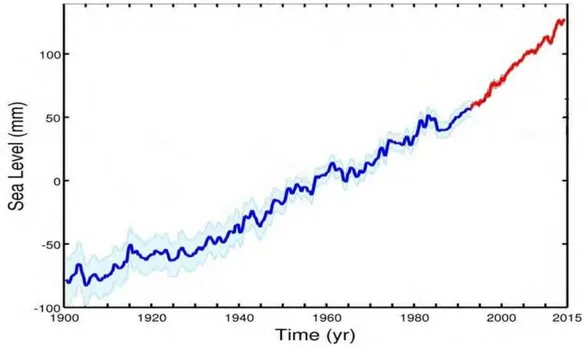
Besides, tide gauge records often have multi-year or multi-decade long gaps. The sparse and heterogeneous coverage of tide gauge records, both temporally and geographically poses a problem for estimating reliable historical mean sea level variations (Meyssignac and Cazenave, 2012). Tide gauges measure sea level relative to the ground, hence monitor ground motions in areas subjected to strong natural (Glacial Isostatic Adjustment (GIA), tectonic/volcanic) or anthropogenic (ground water pumping, oil/gas extraction, sediment loading) ground subsidence. Therefore in order to study the absolute sea level change, the ground motion needs to be removed. Note however that for studying local impacts, the total relative sea level change (climatic sea level change plus vertical land motion) needs to be known (See Section 3.2 of Chapter 3). By developing various strategies, several studies (Douglas, 2001, Church and White, 2006, Jevrejeva et al., 2006 Jevrejeva et al., 2008, Church and White, 2011, Wöppelmann et al., 2007, Wöppelmann et al., 2009) have provided tide gauge based reliable historical sea level time series. In spite of the various approaches used, the results based from these studies are homogeneous and give a mean 20th century sea level rate in the range of 1.6-1.8 mm/yr. Fig.1.3 displays the 20th century global mean sea level curve of Church and White 2011 from tide gauge based past sea level reconstruction (in blue) with the satellite altimetry based sea level curve superimposed in red.
Figure 1.3: 20th century sea level curve (in blue) from tide gauge based past sea level reconstruction of Church and White, 2011and altimetry-based sea level curve (in red) between 1993 and 2015 from AVISO.
10
1.2.2 Satellite altimetry
Since the early 1990s, high precision satellite altimetry record provides nearly global sea level measurements at regular time intervals (Fu and Cazenave, 2001, Church et al., 2013). Chapter 2 of this manuscript discusses the evolution of satellite altimetry, principle of sea surface height (SSH) measurement and the various geophysical and instrumental corrections involved in the precise SSH measurement in detail. The precision of individual SSH measurements based on the various satellite missions has now reached 1-2 cm. Although there are slight differences at interannual time scales in the altimetry-based global mean sea level time series produced by different groups (Masters et al., 2012, Henry, 2014, Dieng et al., 2015), there is very good agreement on the 22 year long global mean sea level trend. Over 1993-2015, the multi-satellite altimetry based global mean sea level rate amounts to 3.3 mm/yr. Precision on the global mean sea level rate is in the order of 0.4-0.5 mm/yr which is derived from assessments of all sources of errors affecting the altimetry measurements (Ablain et al., 2009, Ablain et al., 2015) and from tide gauge comparisons (Beckley et al., 2010, Nerem et al., 2010). Fig.1.4 displays the satellite-altimetry based global mean sea level curve obtained from Archiving Validation and Interpretation Satellite Oceanographic (AVISO) center (same as the red curve in Fig.1.3 but enlarged). The altimetry based sea level curve displays a quasi-linear increase over 1993-2015 with temporary interannual anomalies associated with El Niño (1997/1998) and La Niña (2007/2008, 2010/2011) events (e.g. Nerem et al., 2010). The altimetry-based global mean sea level rate of 3.3 mm/yr over 1993-2015 is significantly higher than the mean rate recorded by tide gauges over the 20th century, suggesting sea level rise acceleration since the two recent decades (Church et al., 2013, Merrifield et al., 2009).
11
Figure 1.4: Altimetry-based global mean sea level temporal curve since 1993. The post glacial rebound correction of -0.3mm/yr has been applied and the annual, semi-annual signals have been removed. A 6 month filter has been applied on the red curve.
1.3 Contributors to global mean sea level rise during the
instrumental era
The two main causes of global mean sea level change are the thermal expansion /contraction of the sea waters in response to ocean warming and the addition of freshwater to ocean basins as a result of land ice loss and water exchange with terrestrial reservoirs (soil and underground reservoirs, lakes, snowpack, etc.).
1.3.1 Ocean temperature and salinity changes
Anomalies in temperature and salinity in the ocean water column change density, which further gives rise to sea level variations (classically called steric variations, or thermosteric or halosteric if associated with only temperature or salinity variations respectively, Cazenave and
12
Llovel, (2010)). Analyses of in situ hydrographic measurements collected by ships over the past
50 years and recently by Argo profiling floats indicate that in terms of global mean, the oceans have warmed significantly since 1950. Over the 1971-2010 period, the 5th Assessment Report of the Intergovernmental Panel on Climate Change (IPCC AR5) shows that the global mean thermosteric sea level (including estimates of deep ocean contribution) trend amounts to 0.8±0.3 mm/yr accounting for about 40% of the observed sea level rise. Over the altimetry period of 1993-2010, the thermosteric sea level trend amounts to 1.1±0.3 mm/yr accounting for about 35% of the total observed sea level rise (Church et al., 2013). Assuming constant total salt content, density changes arising from redistribution of salinity by ocean circulation (halosteric effect) has almost no effect on global mean sea level, although it plays a role at regional scales (Antonov et
al., 2002, Wunsch et al., 2007, von Schuckmann et al., 2009, Cazenave and Llovel, 2010, Stammer et al., 2013, Church et al., 2013, Durack et al., 2014). For example, for the period
1955-2003, Ishii et al., (2006) estimated a halosteric sea level rate of 0.04±0.02 mm/yr. While it is of interest to quantify this effect, only about 1% of the halosteric expansion contributes to the global sea level rise budget. This is because the halosteric expansion is nearly compensated by a decrease in volume of the added freshwater when its salinity is raised (by mixing) to the mean ocean value; the compensation would be exact for a linear state equation (Gille, 2004, Lowe and
Gregory, 2006). Hence, for global sums of sea level change, halosteric expansion cannot be
counted separately from the volume of added land freshwater (Solomon et al., 2007, Church et
al., 2013).
1.3.2 Glaciers melting
Being very sensitive to global warming, observations have indicated that since 1970s, mountain glaciers and ice caps are retreating and thinning with noticeable acceleration since the early 1990s. They represent another significant source of freshwater mass to be added to world’s oceans thereby raising sea level (Church et al., 2013, Gardner et al., 2013, Vaughan et al., 2013). Contribution of glacier ice melt to sea level has been estimated through mass balance studies of a large number of glaciers (Marzeion et al., 2014, Gregory et al., 2013, Church et al., 2013, Leclercq et al., 2011, Church et al., 2011, Cogley, 2009, Meier et al., 2007, Kaser et al., 2006). The mass balance estimates are either based on in situ measurements (monitoring of the annual mean snow accumulation and ice loss from melt) or geodetic techniques (measurements
13
of surface elevation and area change from airborne altimetry or digital elevation models,
Vaughan et al., 2013). The sea level contribution of all glaciers excluding those surrounding the
periphery of Greenland and Antarctica ice sheets has been estimated as 0.62±0.37 mm/yr sea level equivalent (SLE) for 1971-2009 in IPCC AR5. For 1993-2009, its contribution amounts to 0.76±0.37 mm/yr, around 25% of the total observed sea level rise (Church et al., 2013, Church et
al., 2011).
1.3.3 Ice sheets
The mass balance of ice sheets is a topic of considerable interest in the context of global warming and sea level rise since it is expected that if totally melted, Greenland and West Antarctica would raise sea level by several meters. While little was known on the mass balance of ice sheets before the 1990s mainly because of inadequate observations, since then, different remote sensing techniques (e.g. airborne and satellite radar and laser altimetry, Synthetic Aperture Radar Interferometry-InSAR) and space gravimetry since 2002 (Gravity Recovery and Climate Experiment-GRACE) have enabled the monitoring of ice sheet mass balance. Mass balance estimates from data obtained through the various techniques unambiguously show an accelerated ice mass loss from both the ice sheets in the recent years (Hanna et al., 2013,
Gregory et al., 2013, Fettweis et al., 2013, Church et al., 2011, Chen et al., 2009, Velicogna,
2009, Rignot et al., 2008, Hanna et al., 2008 and Vaughan et al., 2013 for a review). During 1993-2003, the IPCC AR5 synthesis has shown that only around 13.5% of the total observed sea level rise was explained by the ice sheet mass loss. However, since then this contribution has augmented resulting in approximately 40% during 2003-2004 showing that this is not constant through time. Over the entire 1993-2009 time period, the ice sheet mass loss contribution to sea level was estimated to be 0.7±0.4 mm/yr SLE, that is, ~ 25% of the total observed sea level rise. Of the total ice mass loss contribution, 0.4±0.2 mm/yr SLE and 0.3±0.2 mm/yr SLE were contributed by Greenland and Antarctica respectively (Church et al., 2013).
1.3.4 Land waters
Changes in water storage on land in response to climate change and variability (i.e., water stored in rivers, lakes, wetlands, aquifers and snow pack at high latitudes and altitudes) and from direct human-induced effects (i.e., storage of water in man-made reservoirs along rivers and
14
ground water pumping) have the potential to contribute to sea level change (Milly et al., 2010). Estimates of climate-related changes in land water storage over the past few decades rely on global hydrological models due to inadequate observational data. Based on hydrological modelling, Milly et al., (2003)and Ngo-Duc et al., (2005) found no long term sea level trend associated with natural land water storage change but interannual to decadal fluctuations, equivalent to several millimeters of sea level. Furthermore, recent studies (Cazenave et al., 2014,
Fasullo et al., 2013, Boening et al., 2012, Cazenave et al., 2012, Llovel et al., 2011, Nerem et al.,
2010) have shown that interannual variability in observed global mean sea level correlates with El Niño Southern Oscillation (ENSO) indices and is inversely related to ENSO-driven changes of terrestrial water storage. While climate-related changes in land water storage do not show significant long-term sea level trends for the recent decades, direct human (anthropogenic) interventions in land water storage (reservoir impoundment and groundwater depletion) have each contributed at least several tenths of mm of sea level change (Church et al., 2013, Konikow, 2013, Pokhrel et al., 2012, Wada et al., 2012, Konikow, 2011, Milly et al., 2010, Chao et al., 2008). Reservoir impoundment causes a sea level decrease whereas ground water depletion increases the sea level since most of the water extracted from the ground ends up in one form or another into the oceans. Reservoir impoundment exceeded groundwater depletion for the majority of the 20th century but groundwater depletion has increased and now exceeds current rates of impoundment, contributing to an increased rate of global mean sea level rise. IPCC AR5 estimated the net anthropogenic contribution of land waters to sea level to be 0.12±0.1 mm/yr for 1970-2010. Over 1993-2010, its contribution amounts to 0.38± 0.12 mm/yr, around 12% of the total rate of observed sea level rise (Church et al., 2013).
Fig.1.5 (adapted from Meyssignac and Cazenave, 2012) compares the observed global mean sea level rise to different components and their sum over the altimetry era.
15
Figure 1.5: Observed sea level from satellite altimetry over 1993–2010 (blue solid curve; thermal expansion (red curve; mean value based on temperature data from Levitus et al., 2009; Ishii and Kimoto, 2009); contribution from Greenland and Antarctica (cyan curves) and glaciers (green curve). The black curve represents the total land ice contribution while the blue dotted curve represents the total climatic contribution (sum of thermal expansion and land ice) (from Meyssignac and Cazenave, 2012).
1.4 Thesis objectives
Sea level is an integrated climate parameter that involves interactions of all components of the climate system (oceans, ice sheets, glaciers, atmosphere, and land water reservoirs) on a wide range of spatial and temporal scales. In the previous sections, we discussed the evolution of global mean sea level over various time scales, factors contributing to global mean sea level changes. Considering the highly negative impact of sea level rise for society, the multidisciplinary aspects of sea level rise remain a major focus of climate research. Monitoring sea level change and understanding its causes has considerably improved in recent years owing to the advent of precise in-situ and remote sensing observations. My thesis contributes to a better estimation and understanding of sea level changes not only at a global scale for the recent decade but also most importantly focusses on regional sea level variability as regional sea level can
16
substantially deviate from the global mean and can vary on a broad range of spatial and temporal scales. The main objectives and the organization of the thesis are outlined below.
Chapter 2 of this thesis presents two main works that involve the validation of sea level variations measured by the most recent satellite altimetry mission and the global mean sea level closure budget for the recent decade using various observational data.
In the first part of this chapter, we provide a detailed description on the evolution of different altimetry satellites since the beginning of the altimetry era, principle of SSH measurement and the various geophysical and instrumental corrections involved in the precise SSH measurement. This is then followed by the validation of sea level variations measured by SARAL-AltiKa by comparing them with SSH measurements from JASON-2 and various available tide gauge records. The second part of the chapter attempts to answer the following questions: Can the global mean sea level budget be closed using available observational datasets of sea level and its contributing components over 2003-2012? If not, can the significant residual signal be possibly related to deep ocean contribution and/or signal that corresponds to regions that are not monitored by observing systems or uncertainties in data processing?
Chapter 3 deals with regional sea level variability, its causes and estimates of total relative sea level change at various vulnerable regions of the world.
In the first part of the chapter, climate-related and non-climatic causes of regional sea level variability over the altimetry era (1993-2013) are discussed in detail. In the second part of the chapter, we then focus our interest on long-term (i.e. at least 60 years) regional sea level variability. By making use of a two dimensional past sea level reconstruction and long term in-situ steric sea level data, the causes of regional sea level variability over 1950-2009 in the Indian Ocean, South China Sea and Caribbean Sea are first discussed. Furthermore, estimates of total relative sea level change (sea level change as felt by the population) since 1950 at several tide gauge locations at the vulnerable coasts and islands of the above mentioned regions obtained using a multidisciplinary approach as in Becker et al., (2012) are then discussed and compared. In the final chapter (Chapter 4) we discuss the role of ocean dynamics, internal climate variability and external forcing on regional sea level variability with a special focus on the Pacific Ocean (especially the western tropical Pacific) where the regional sea level trends since the two recent decades are estimated to be three times the global mean sea level rate. This chapter has various sections. The first two sections are dedicated to various well known internal
17
unforced climate modes and two main sources of externally forced climate variability. This is then followed by a section that focusses on detection and attribution of climate change on global and regional sea level variability where a review of various studies on this subject is performed. The next section focusses on the Pacific Ocean sea level spatial trend patterns over the altimetry era. The contribution of internal climate modes and ocean dynamic processes to the Pacific Ocean sea level trend pattern estimated using observation in-situ data is first discussed. The presence of anthropogenic sea level fingerprint in the Pacific Ocean sea level since 1993 is also studied using observational altimetry and phase 5 of Coupled Model Inter-comparison Project (CMIP5) climate model-based sea level data.
19
Chapter 2
Multi satellite altimetry record and global
mean sea level budget
Satellite altimetry missions have transformed the way we view Earth and its ocean and has been the main tool for continuously and precisely monitoring the sea surface height (SSH) with quasi-global coverage and short revisit time. In Chapter 1, we have seen the evolution of global mean sea level (GMSL) as measured by satellite altimeters since 1993. In this chapter, we first discuss the evolution of various altimetry satellites used for ocean observation, principle behind the altimetry-based SSH measurement and different error corrections involved in precise SSH measurements. We then move on to the estimation of global mean sea level budget since a decade using various observational and in-situ data.
2.1 Evolution of altimetry satellites
Satellite altimetry was developed in the 1960s soon after the flight of artificial satellites became a reality (Fu and Cazenave, 2001). The first altimetry satellite, GEOS 3 (Geodynamics Experimental Ocean Satellite) was launched in 1975 and carried instruments to yield useful measurements of sea level and its variability. However, its performance was not good enough to extract useful scientific information from its measurements. This was then followed by Seasat (SEA faring SATellite) and Geosat (GEOdetic SATellite) missions in 1978 and 1985 respectively. While Seasat gave us the first global view of ocean circulation, waves and winds, Geosat was the first mission to provide long-term (over 3 years) of high quality altimetry data. However, until the early 1990s, satellite altimetry has been more useful to marine geophysics rather than oceanography. This is mainly because the orbital error (see section 2.1.2 for details)
20
for these missions was so large (from several decimeters to ~1m) that the altimetry range uncertainty prevented detection and precise measurements of phenomena associated with ocean dynamics such as dynamic topography, tides, sea level etc. (Fu and Cazenave, 2001, Palanisamy
et al., 2015a).
The era of precise satellite altimetry dedicated to space oceanography began in the early 1990s with the launch of ERS-1, a European Space Agency (ESA) mission in 1991 and the National Aeronautics and Space Agency (NASA)/ Centre National d’Etudes Spatiales (CNES) joint venture TOPEX/Poseidon in 1992. In fact, TOPEX/Poseidon revolutionized the study of Earth’s oceans by providing the first continuous, global coverage of ocean surface topography. Its data made a huge difference in our understanding of the oceans and their effect on global climatic conditions. Its repeat cycle (i.e. the time taken for the satellite to pass vertically over the same location) of ~10 days provided more information than in-situ measurements over hundred years. The mission far exceeded the expectations in terms of both mission duration (initial design life was 5 years but stayed in operation for 13 years) and measurement system performance (Buis
et al., 2006).
During the period of TOPEX/Poseidon (1992-2006), several other new altimetry missions were launched: ERS-2 (ESA, 1995-2011), Jason-1 (NASA/CNES, 2001-2012), ENVISAT (ENVIronmental SATellite, ESA, 2002-2012) and Jason-2 (NASA/CNES, 2008- ). The combination of several satellites available at the same time enabled a good compromise between the spatial and temporal resolutions for ocean monitoring. For example, while the repeat cycle of TOPEX/Poseidon was ~10 days (good temporal resolution), its inter-track spacing at the Equator was in the order of 315 km; whereas in the case of ENVISAT, its repeat cycle was 30 days with inter-track spacing in the order of 80 km at the Equator (good spatial resolution). Moreover, while TOPEX/Poseidon, Jason-1 and Jason-2 flew at the non- sun synchronous orbit (up to 66°N/S), ENVISAT’s polar sun synchronous orbit further enabled high latitude ocean coverage (up to 81.5° N/S) thereby complementing to the other existing missions.
Cryosat-2 and HY-2A are two other satellite altimetry missions launched by ESA and China in 2010 and 2011 respectively. The Cryosat-2 orbit at an inclination of about 92 degree and an altitude of 717 km covers almost all the polar region and henceforth is dedicated to polar observation while HY-2A at sun synchronous and geodetic orbit helps in monitoring the
21
dynamics of the ocean. Since the beginning of 2013, a new altimetry mission, SARAL-AltiKa, a joint venture between CNES and Indian Space Research Organization (ISRO), now ensures the continuity of high precision sea level data along with the existing Jason-2 measures (Verron et
al., 2015). It is the first oceanographic mission using a high frequency Ka band altimeter for
improved spatial and temporal resolution and flies in the same orbit as that of ENVISAT (a detailed explanation on SARAL-AltiKa is presented in Section 2.1.4). Another mission, Jason-3 in the framework of a co-operation between CNES, NASA, Eumetsat (EUropean METeorology SATellite) and NOAA (National Oceanic and Atmospheric Administration) is proposed to be launched soon. This mission is similar to those of TOPEX/Poseidon, Jason-1 and Jason-2 with the same kind of payload and orbital parameters.
Since satellite altimetry has proven to be a valuable source of data for ocean monitoring and understanding, several future missions are foreseen such as Sentinel-3 Jason-CS, SWOT (Surface Water Ocean Topography). Continuous monitoring with the help of such satellite altimeters will further enhance our understanding of oceans and their mechanisms.
2.1.1 Principle of satellite altimetry
The radar altimeters on board the satellite transmit signals at high frequency (over 1700 pulses per second) towards the sea surface which is partly reflected back to the satellite. Measurement of the round-trip travel time is then converted to obtain the distance of the satellite above the instantaneous sea surface, called as ‘range’. SSH measurement is deduced from the difference between the satellite distance to the Earth’s centre of mass (deduced from precise orbitography and called ‘satellite/orbit altitude’) and the satellite distance (range) above the sea surface (Fig.2.1) Besides sea surface height, wave height and wind speed over the oceans can also be measured from the amplitude and waveform of the return signal.
2.1.2 Corrections involved in Sea Surface Height measurement
The determination of precise SSH measurements from satellite altimetry is influenced by many factors. Amongst the most important are sensor characteristics, long-term stability of the altimeter, and the methods used in altimeter data processing (Fernandes et al., 2006). While the sensor characteristics of the altimeter are pre-determined depending on the altimetry missions,
22
instrumental and orbital errors, differences in the methodology for processing altimetry data and the corrections involved are crucial for sea level monitoring. High precision SSH measurements require (1) precise orbit determination of the satellite and (2) application of accurate geophysical, corrections to the raw altimetry signal. The latter accounts for the interactions of altimeter signal with the atmosphere and sea surface. Slight differences in the models used or processing approaches for the above mentioned corrections can seriously impact the SSH estimates and corresponding uncertainties. Therefore, from Section 2.1.1, the precise SSH measurement from satellite altimetry can now be expressed as
SSH = S – R – Corrections + ε (2.1)
where,
S = Orbit altitude
R = Range
Corrections = (orbital + propagation + geophysical + surface) corrections
ε = remaining random and systematic errors
23
In this section, we discuss several of these corrections involved for precise SSH estimation.
1) Orbital correction
The quality of the altimetry data depends on the ability to precisely determine a satellite’s position on orbit. Orbital error is caused by imperfect knowledge of the spacecraft position in the radial orbit direction and is the largest error source on altimetry measurements for SSH monitoring. Therefore, a very precise knowledge of the satellite orbit with respect to Earth’s reference ellipsoid is essential. The satellite’s orbit can be also perturbed by gravitational forces related to the non-uniform distribution of Earth’s gravity field, and those caused by the sun, moon and other planets. Forces on the satellite’s surface such as atmospheric drag (e.g. low orbit satellites experience more atmospheric drag) and radiative pressure (e.g. solar radiation, Earth’s IR radiation etc.) also play a role in the perturbation of the satellite’s orbit. This indicates that a detailed knowledge of the satellite and its variations due to maneuvers, fuel consumption, solar panel orientation etc. are also necessary in order to precisely model the above mentioned forces acting on it. Precise orbit determination is done through a combination of satellite tracking and dynamic modelling. Satellite tracking in general involves the use of Satellite Laser Ranging (SLR), Global Positioning System (GPS) and Doppler Orbitography and Radio positioning System (DORIS). A dynamical model taking into account the forces acting on the satellite is then fitted through the tracking data to obtain the precise orbit of the satellite.
2) Propagation corrections
As the radar altimetry signal travels through the atmosphere to the sea surface, it is slowed down due to the presence of various elements in its path. The delay in the propagation of the radar signal thus needs to be corrected in order to estimate the precise range, i.e. the distance between the satellite and sea surface. There are three types of propagation delays that need to be accounted for: (1) ionospheric, (2) wet and (3) dry tropospheric corrections.
a) Ionosphere correction
This correction takes into account the path delay in the radar signal due to the presence of electrons in the ionosphere. The ionosphere is the uppermost layer of the atmosphere (ranging between 60 and 800 km) and the electrons are produced as a result of ionization attributed to solar radiation. As a result, it causes the altimeter to slightly over estimate the range by 1 to 20
24
cm. This amount can vary with respect to the seasons, solar cycle and occurrences of geomagnetic storms with the maximum influence occurring at the tropical band. Since the range delay due to the presence of electrons is related to electromagnetic radiation frequency, the correction can be estimated using two different radar frequencies (for example, C-band and Ku -band for TOPEX and Jason-1). This correction can also be taken into account from models of the vertically integrated electron density (Fu and Cazenave, 2001, Callahan, 1984, Imel, 1995).
b) Wet troposphere correction
The wet tropospheric correction is the correction for the delay of the radar signal due to the presence of water vapor content in the atmosphere. This is a difficult correction to be accounted for as the wet atmospheric effect highly varies both spatially and temporally with maximum occurring in the tropical convergence zones and magnitudes ranging from 5cm to 30 cm. Over the oceans, the wet tropospheric correction is in general computed using on-board microwave radiometer measurements. But, such radiometric measurements generally fail near the coasts where the signal coming from the surrounding land surface contaminates the radiometer measurements (Desportes et al., 2007). In such cases, the correction is computed from meteorological model outputs such as ECMWF (European Center for Medium Range Weather Forecast) or NCEP (National Centers for Environmental Prediction) models (Legeais et
al., 2014).
c) Dry troposphere correction
The mass of dry air molecules in the atmosphere causes a range delay known as the dry tropospheric effect. It is directly proportional to sea level pressure and is the largest adjustment that has to be applied to altimetry measurement as its order of magnitude is about 2.3m. However, its temporal variations are low and range a few centimeters only. The dry tropospheric correction is computed using atmospheric model pressure forecasts such as ECMWF.
3) Geophysical corrections
The gravity forces generated by the Sun and Moon on the Earth can create perturbations on the earth’s interior and also sea surface elevations of few meters. These geophysical effects are called as tidal effects and can be classified into four types: (1) ocean, (2) solid Earth, (3) polar tidal and (4) loading effects.
25
a) Ocean, solid Earth tidal and loading corrections
Ocean tides and their variations are the result of the combined attraction of Sun and Moon and represent more than 80% of the surface variability in open ocean. The tidal periods (half a day or one day) are shorter than the repeat periods of an altimetry satellite. Tidal correction is therefore essential since they contaminate the low frequency altimetry signals. Furthermore, for the estimation of dynamic sea surface height, the magnitude of ocean tides are very large and must therefore be removed as they are considered as noise. Ocean tidal corrections are performed using assimilated hydrodynamic and statistical models that estimate tides globally with high spatial resolution (Fu and Cazenave, 2001, Ray, 1999).
The gravitational attraction of the Sun and Moon also impacts Earth’s interior causing the surface of the Earth beneath the ocean to be slightly deformed. This is called as the solid Earth tidal effect. This effect is nearly in phase with the ocean tide and is corrected using models.
Furthermore, the change in the weight of the water column due to variations in tides causes an elastic loading effect on the sea floor that is also corrected using models.
b) Polar tidal correction
The axis of rotation of the Earth deviates slightly from the Earth’s ellipsoidal axis over a period of several moths annually. This as a result causes variations to both solid Earth and oceans and is called as polar tidal effect (Desai, 2002, Wahr, 1985). The polar tide correction is implemented through modelling that requires precise knowledge on the Earth’s axis of rotation. 4) Surface corrections
Apart from propagation and geophysical corrections applied to altimetry signal, there are two types of surface corrections that need to be accounted for: (1) inverse barometric and (2) sea state bias corrections.
a) Inverse barometric (IB) correction
The response of the sea surface to changes in atmospheric pressure has a large effect on measured sea surface height as the ocean responds directly to atmospheric pressure changes. Sea level falls (rises) as the atmospheric pressure loading increases (decreases). For example, an increase in the atmospheric pressure by 1mbar pushes the sea level down by 1 cm. This is called as the isostatic inverse barometric effect (Wunsch and Stammer, 1997, Ponte and Gaspar, 1999,
26
Carrère and Lyard, 2003). The magnitude of the IB effect can reach up to ± 15 cm and is
corrected using meteorological models such as ECMWF.
b) Sea State Bias (SSB) correction
This correction includes the electromagnetic bias (EM bias) and skewness bias. The EM bias is the correction for bias in measurements due to varying reflectivity of the wave troughs and crests (Chelton, 1994). The concave form of wave troughs tends to concentrate and reflect the altimetry signal better than the wave crests that disperse the signal. Therefore the altimetry signal return from the troughs is stronger than from the crests. Furthermore, in the case of wind waves, the wave troughs have a larger surface area than the pointy crests and this is called as skewness bias. Both the EM and skewness bias causes the mean reflecting surface to be shifted towards the troughs. They vary with increasing wind speed and wave height. SSB is estimated using empirical formulas derived from altimeter data analysis and models (Tran et al., 2006). The range correction varies from a few to 30 cm.
5) Other potential errors
Other sources of potential errors in SSH measurements include altimeter instrumental ageing errors. Altimeter parameters are precisely monitored over all the mission life-time to detect instrumental anomalies (Ablain et al., 2009). Based on the instrumental anomalies observed in the satellites, corrections such as for centre of gravity, waveforms etc. are applied.
Over the years, technological developments have considerably decreased the instrumental error down to 1.7 cm for TOPEX/Poseidon and even lesser for Jason-1/2 and other recent missions. Similarly improved satellite orbit determination has reduced the root-mean-squared (rms) orbit error down to the range of 1-2 cm for Jason-1/2. Fig.2.2 displays the evolution of altimetry instrumental and orbital errors. Owing to internationally concerted effort in improved estimates of the geophysical and environmental corrections, the rms error of the various corrections has now been reduced down to ~2.7 cm for a single SSH measurement.
27
Figure 2.2: Evolution of orbital and instrumental errors in satellite altimetry (Source: AVISO-CNES)
2.1.3 Multi-mission SSH altimetry data
We carried out global and regional sea level studies by making use of multi-mission merged SSH altimetry data. The purpose of using multi-mission altimetry data is to obtain the most stringent accuracy requirements that are needed for climate research. Moreover, as mentioned in Section 2.1, the combination of several satellites enables a better compromise on spatial and temporal resolution. Merging multiple altimeter data sets is not easy. It requires homogenous, inter-calibrated data sets; correcting of orbit error for the less precise altimeter missions; extracting the sea level anomaly using a common reference surface; and combining the data through a mapping (or assimilation) method (Le Traon et al., 1998). After calculating the along track sea level measures for each of the satellite missions, the main steps consists of: combining all missions together, reducing the orbit and the long wavelength errors, computing the gridded sea level anomalies using an objective analysis approach (Ducet et al., 2000, Le
Traon et al., 2003), and generating mean sea level products (e.g. GMSL time series, gridded sea
level time series) dedicated for climate studies (Ablain et al., 2015). Owing to the homogenization of the altimetry corrections between all the missions, the uncertainty in multi-mission GMSL trend over 1993-2010 is now reduced to 0.5 mm/yr. The main source of this error
28
remains to be the wet tropospheric correction with a drift uncertainty in the range of 0.2-0.3 mm/yr (Legeais et al., 2014). Orbit error and altimeter parameters error also add an uncertainty in the order of 0.1 mm/yr. Furthermore, imperfect links between various altimetry missions cause a GMSL trend error of about 0.15 mm/yr (Ablain et al., 2015).
2.1.4 SARAL-AltiKa, the new altimetry mission
SARAL-AltiKa mission, launched in February 2013, is an answer to the needs of the oceanographic community, continuity of high accuracy, high resolution, near-real time observations of the ocean surface topography as at least 2 simultaneous altimetry missions are required to fulfill this need. As a consequence, along with the existing Jason-2, SARAL-AltiKa mission is considered as ‘gap filler’ between ENVISAT (lost in April 2012) and Jason-3/Sentinel-3 (expected in 2015; Verron et al., 2015). This is the first oceanographic mission that uses a high frequency Ka band altimeter (frequency and bandwidth of 35.75 GHz and 500 MHz). The main objective of this mission is to help the oceanographic community to improve knowledge on the ocean meso-scale variability, a class of high energy processes with wavelengths in the range of 50 km to 500 km (Verron et al., 2015). The Ka band frequency of SARAL-AltiKa improves spatial and temporal resolution and thus enables a better observation of the ocean at meso-scale. It is also well suitable for studying mean sea level variations, sea and land ice, wave heights and coastal dynamic processes (as SARAL-AltiKa can reach as close as 8km to the coasts while Jason-2 has managed only up to 15 km), as well as continental water bodies like rivers, lakes, wet lands, etc. (Palanisamy et al., 2015a). Furthermore, SARAL-AltiKa flies at an almost polar (final inclination at 98.55°) sun-synchronous orbit as that of ENVISAT. This enables better observation of polar ice and oceans. With a repeat cycle of 35 days (similar to ENVISAT), SARAL-AltiKa provides a high resolution coverage of the oceanic domain with an inter-track spacing at the equator of 75 km.
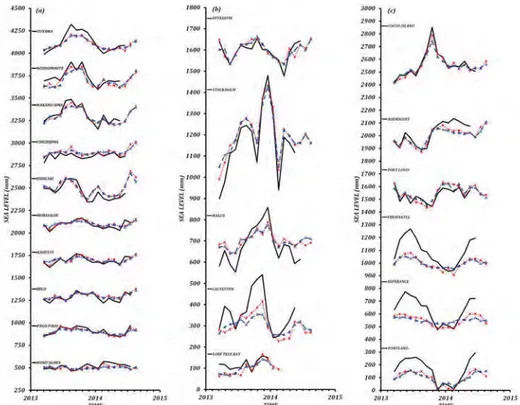
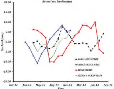
In our study, we performed a global and regional validation of the sea level variations measured by SARAL-AltiKa by comparing it with Jason-2 and tide gauge records. This has been published as an article titled ‘Sea level variations measured by the new altimetry mission SARAL-AltiKa and its validation based on spatial and temporal curves using Jason-2,tide gauge data and an over view of the annual sea level budget’.