Université de Montréal
A Sensitivity Analysis of Cross-Country Growth Regressions:
Is 1990-2010 Different?
par
Rami KIWAN
Département de sciences économiques
Faculté des arts et des sciences
Mémoire présenté à la Faculté des arts et des sciences
en vue de l’obtention du grade de maîtrise
en sciences économiques
décembre, 2012
Université de Montréal Faculté des arts et des sciences
Ce mémoire intitulé :
A Sensitivity Analysis of Cross-Country Growth Regressions: Is 1990-2010 Different?
présenté par :
Rami KIWAN
a été évalué par un jury composé des personnes suivantes :
Benoît Perron Président-rapporteur Emanuela Cardia directrice de recherche François Vaillancourt membre du jury
Abstract
This paper examines the robustness of explanatory variables in cross-country growth regressions. It employs a variant of Leamer’s (1983, 1985) extreme-bounds analysis. My results confirm Levine and Renelt’s (1992) conclusion, but identify more variables to be robustly correlated with economic growth. Of 25 explanatory variables tested, I find 8 to be significantly and robustly correlated with long-term growth over the 1990-2010 period. The strongest evidence is for the investment ratio, government consumption share in GDP, the rule of law, and the Sub-Saharan dummy. I also find strong empirical evidence for conditional convergence, which is consistent with the neoclassical growth model.
Keywords: conditional convergence; cross-country regressions; economic growth; extreme-bounds analysis.
Résumé
Cet article étudie la sensibilité des estimations de certaines variables explicatives de la croissance économique dans des régressions en coupe transversale sur un ensemble de pays. Il applique un modèle modifié de l’analyse de sensibilité de Leamer (1983, 1985). Mes résultats confirment la conclusion de Levine and Renelt (1992), toutefois, je montre que plus de variables sont solidement corrélées à la croissance économique. Entre 1990-2010, je trouve que huit sur vingt cinq variables ont des coefficients significatifs et sont solidement corrélées à la croissance de long terme, notamment, les parts de l’investissement et des dépenses étatiques dans le PIB, la primauté du droit et une variable dichotomique pour les pays subsahariens. Je trouve aussi une preuve empirique solide de l'hypothèse de la convergence conditionnelle, ce qui est cohérent avec le modèle de croissance néoclassique.
Mots-clés : analyse de sensibilité ; convergence conditionnelle ; croissance économique ; régressions en coupe transversale sur un ensemble de pays.
Acknowledgements
I would like to acknowledge and extend my heartfelt gratitude to my advisor, Dr. Emanuela Cardia, who offered her continuous advice and vital encouragement throughout the course of this thesis. In combination with the mentorship of my advisor, I was lucky to work with dynamic and intelligent committee members, Dr. Benoît Perron and Dr. François Vaillancourt, to whom I would like to express my deepest appreciation for their constructive comments and suggestions.
I am grateful to the administrative body in the department of Economics, most especially, to Johanne Ménard-Simard for administrative assistance. I would also like to thank my colleagues in the department for helpful technical tips and lunch discussions. The library staff at the Université de Montréal was of a great help for me, too.
I am indebted to my friends, especially Carrie Mandak for helping with editing. I finally take this opportunity to thank my beloved parents and my family for their regular encouragement and moral support all through the Master’s program.
Table of Content
INTRODUCTION 1
CHAPTER 1 - LITERATURE REVIEW 3
SECTION 1.1 - HISTORICAL OVERVIEW OF MODERN GROWTH THEORY 3
SECTION 1.2 - EMPIRICS OF ECONOMIC GROWTH 8
SECTION 1.3 - A DISCUSSION OF CROSS-COUNTRY GROWTH REGRESSIONS 11
SECTION 1.4 - SENSITIVITY AND ROBUSTNESS 16
CHAPTER 2 - MODEL AND RESULTS 25
SECTION 2.1 - METHODOLOGY AND MODEL 25
SECTION 2.2 - BASELINE REGRESSION AND SOME FIRST RESULTS 30
SECTION 2.3 - FISCAL-POLICY INDICATORS 36
SECTION 2.4 - INTERNATIONAL-TRADE INDICATORS 38
SECTION 2.5 - MONETARY-POLICY INDICATORS 40
SECTION 2.6 - REGIONAL AND GEOGRAPHICAL DUMMIES 42
CONCLUSION 45
DATA APPENDIX 46
List of Tables
Table 1: Breusch-Pagan / Cook-Weisberg test for heteroscedasticity for the baseline regression ... 31
Table 2: The variance inflation factor analysis ... 31
Table 3: Sensitivity results for basic variables ... 34
Table 4: Cross–country averages, 1990–2010a ... 35
Table 5: Cross–country correlations ... 36
Table 6: Sensitivity results for fiscal variables ... 38
Table 7: Sensitivity results for trade variables ... 40
Table 8: Sensitivity results for monetary variables ... 42
Introduction
Economists have long been seeking to comprehend the factors contributing to the enormous gap between rich and poor countries. A better understanding of the relationships between national policies and long-run growth would both contribute to our ability to explain differences between per capita incomes across countries and provide a basis for making policy recommendations that could lead to improvements in economic welfare, especially in poor countries.
Following the seminal work of Kormendi and Meguire (1985), Grier and Tullock (1989), and Barro (1991a), economists have used cross-country regressions to search for empirical linkages between growth rates and policy indicators. The large empirical growth literature has identified over 100 fiscal, monetary, trade, exchange-rate, financial, and geographical explanatory variables to be significantly correlated with long-term growth. Yet, empirical evidence shows that many of these findings are fragile to small alterations in the list of right-hand-side variables.
There is no single consensus of a theoretical framework to guide empirical work on growth. A review of available evidence suggests that the current state of understanding about the sources of growth is relatively poor. Using various econometric techniques to examine empirical linkages between growth and possible explanatory variables, in an attempt to figure out the determinants of growth, has produced results in some studies that are frequently in contradiction with results reported in others. A central question for empirical economic growth in particular is which explanatory variables to include and which to exclude. Which variables are the “real” causes of growth? In which variable should one have more confidence?
Some answers have already been provided. Literature on the sensitivity of estimates in cross-country growth regressions has emerged starting in the 1990s. The objective of this paper is to examine core variables used by other studies in the literature and perform an extensive sensitivity analysis by using a modified version of Leamer’s (1983, 1985) extreme-bounds analysis (EBA). I borrow the context of the empirical model from Levine and Renelt
(1992). I replicate a modified version of the model with recent data over the 1990-2010 period to examine whether using different (mainly due to starting date) periods would necessarily imply different results. I study a large number of variables that have been the focus of attention in a broad array of cross-country growth studies. I, however, should point out that I was limited by the available data, which did downsize the matrix of variables used. Data series for some countries were not complete over the study period, several variables were not available or some databases were not accessible to me.
My findings identify a few more variables to be robustly correlated with growth, as compared to Levine and Renelt (1992). In particular, the average growth rate of real GDP per capita depends negatively on the share of government consumption in GDP and on the ratio of government consumption minus defense spending, and positively on the current account balance share of GDP. In accord with Sala-i-Martin (1997a, b), dummies for Sub-Saharan countries and former French colonies are negatively associated with long-run growth. While several policy-variables tested are not robustly correlated with growth, the growth rate of real GDP per capital depends positively on the investment-to-GDP ratio and on an indicator for the rule of law. I also find strong empirical evidence for conditional convergence, which is consistent with the neoclassical growth model. Perhaps the real surprise is the nonrobust partial correlation between primary-school enrollment rate and growth which is different from previous results in the literature.
Before going further, I should emphasize this paper’s limitations. I do not identify growth determinants, establish causal links, present policy recommendations, or run the full sensitivity analysis test discussed by Leamer. I simply test the robustness of some empirical linkages between policy-variables and growth to small alterations in the conditioning information set.
The rest of the paper is organized as follows. Chapter 1 presents an overview of the economic growth theory and empirics; and discusses the cross-country method along with the two main sensitivity testing approaches used by economists. Chapter 2 describes the model, the methodology, the data set used, in addition to the main empirical results of the paper, and the last chapter concludes.
Chapter 1 - Literature Review
Growth is one of the most important issues economists have tried to study and model in order to understand why one economy grows more than another.1 I will make a brief review of the large body of literature in existence, although the objective of this paper is to examine the sensitivity of estimates in cross-country growth regressions over the period 1990-2010.
The economic growth literature has first emerged with the neoclassical growth model of Solow-Swan in the 1950s and Cass-Koopmans in the 1960s.Yet, the study of economic growth had languished for two decades starting in late 1960s before becoming vigorous again starting in late 1980s with a new research strand, called endogenous growth theory.
Following the introduction of cross-country regressions into growth analysis by the seminal work of Kormendi and Meguire (1985), Grier and Tullock (1989), and Barro (1991a), the empirical literature on the determinants of economic growth has become very large and suggested numerous additional explanatory variables (when added one at a time).
Section 1.1 -
Historical Overview of Modern Growth Theory
Classical economists provided many of the basic ingredients that appear in modern theories of economic growth. These contributions to the neoclassical tradition since the late 1950s include the basic approaches of competitive behavior in equilibrium dynamics, the role diminishing returns and its linkage with the accumulation of physical and human capital, the relation between per capita income and the rate of population growth, the effects of technological shocks, and the role of monopoly power as an incentive for technological advance.
The starting point of modern growth theory is the classic article of Ramsey (1928) A
Mathematical Theory of Saving, as argued by Barro and Sala-i-Martin (2004). Early growth
1
See Barro, Robert J. and Xavier Sala-i-Martin. 2004. Economic Growth. Cambridge, Mass.: MIT Press.page 1,for an illustration of the importance of economic growth by assessing the long-term performance of the U.S. economy.
theories featured a central role for capital accumulation. In the aftermath of the Great Depression, Harrod (1939) and Domar (1946) attempted to integrate Keynesian analysis with elements of economic growth. The Harrod-Domar model posited a linear relationship between investment and growth rates worldwide. It used production functions with little substitutability between the inputs and argued that the capitalist system is intrinsically unstable.2
The more important contributions during this era were those of Solow (1956) and Swan (1956). The Solow-Swan model suggested that growth rates were dependent, not on investment, but on the rate of technological change. The model adopted the neoclassical form of the production function with constant returns to scale, diminishing returns to each input, and positive elasticity of substitution between the inputs. Despite its simplicity, the Solow-Swan model has many predictions. A basic property of the Solow-Solow-Swan model is the concept of conditional convergence: the lower the starting level of real per capita gross domestic product (GDP), relative to the steady-state position, the higher (or the faster) the predicted growth. The convergence is conditional because the steady-state levels of capital and output per worker depend (positively) on the saving rate, (negatively) on the growth rate of population, and on the position of the production function—all might vary across economies because of the absence of substantial labor mobility. Barro (1991a, p. 407) argues that “The main element behind the convergence result in neoclassical growth models is diminishing returns to reproducible capital.” Poor countries tend to grow at high rates because they have low ratios of capital to labor and, thus, high marginal products. Nonetheless, this property has not been exploited as an empirical hypothesis for economic growth across countries until the late 1980s and has had high empirical explanatory power ever since. Empirical studies suggest additional sources of cross-country variation; e.g. differences in government policies and in initial stocks of human capital (Barro (1991a)).
Another prediction of the Solow-Swan model is that the per capita growth rate of the steady-state income depends only on the rate of technological progress—it must eventually cease, in the absence of continuing improvements in technology. Yet, it gives us little notion
2 Years later, Domar himself will argue that his model was not appropriate for determining long-term growth
of what might determine technological progress, especially when technology must be conceived to include all aspects of social organization that might relate to the effectiveness of production (Hoover and Perez (2004)).
According to the Solow-Swan model, the steady-state capital-to-income ratio is constant, since both variables grow at the same rate. In addition, the marginal product of capital is constant, while the marginal product of labor grows at the rate of technological progress. Mankiw et al. (1995) suggest that these predictions are “broadly consistent with experience”. They argue that the U.S. capital-to-income ratio exhibits little trend and the real wage grows at the same rate as income per person, while in cross-country data, income per capital is positively correlated with saving rates and negatively correlated with population growth rates, and these correlations are “quite strong”.
In an attempt to reconcile the theory with a positive, possibly constant, per capita growth rate in the long run while retaining the prediction of conditional convergence, the models of the 1950s and 1960s assumed that technological progress is exogenous. The long-run per capita growth rate in these models is determined entirely by the rate of technological progress, which is outside the model, in addition to the exogenous growth rate of population; “Thus we end up with a model of growth that explains everything but long-term growth, an obviously unsatisfactory situation”, as argued by Barro and Sala-i-Martin (2004, p. 18). Koopmans (1963) and Cass (1965) brought Ramsey’s treatment of household optimization back into the neoclassical growth model and thereby provided for an endogenous determination of the saving rate. These models as well tend to preserve the hypothesis of conditional convergence, but this endogeneity of saving “does not eliminate the dependence of the long-run per capita growth rate on exogenous technological progress”, as argued by Barro and Sala-i-Martin (2004, p. 18).
After the work of Koopmans (1963) and Cass (1965) completed the basic neoclassical growth model, growth theory became excessively technical and thereby steadily lost contact with empirical applications. In contrast, development economists tended to use technically unsophisticated but empirically useful models—unsurprisingly, since their profession consists
of giving advice to countries.3 As Barro and Sala-i-Martin (2004) point out, the fields of economic development and economic growth drifted apart, and the two areas became almost completely separated.
Because of this lack of empirical evidence, research on growth theory shrunk considerably on the eve of the rational-expectations revolution, incorporated by Lucas (1972, 1976) into macroeconomics, and the oil shocks in 1973-1975. For the next 15 years or so, macroeconomic research focused on short-term fluctuations. Major contributions included the incorporation of rational expectations into business-cycle models, and improved approaches to policy evaluation, like the application of general-equilibrium methods to real business-cycle theory (RBC).
The next half of 1980s witnessed a reorientation of macroeconomic research programs away from the study of short-run cycles back to economic growth. The neoclassical model was largely abandoned in favor of what became known as endogenous growth theory, in which the rate of technological change varied across countries depending on other factors than those addressed by the neoclassical model. The field experienced a boom, beginning with the work of Romer (1986, 1987), Lucas (1988), Barro (1991a, b), and Rebelo (1992). Despite the variety of topics these models tackled, this shift happened for two widely shared reasons:
a) A recognition of the significance of long-run growth; and
b) A reject of the restriction brought by neoclassical growth model in which the long-term per capita growth rate was pegged by the rate of exogenous technological progress. These recent contributions determine the long-run growth rate within the model—hence, the designation endogenous growth models—and growth may go on indefinitely. These models, as argued by Hoover and Perez (2004), “give little guidance as to which of the many possible factors really influence growth.” Substantial room remains for theory to be informed by empirical investigations.
3
The World Bank’s RMSM, developed in 1972, was based on Harrod-Domar. For more details see Kenny, Charles and David Williams. 2001. "What Do We Know About Economic Growth? Or, Why Don't We Know Very Much?" World Development, 29(1), 1-22.
Recent work on endogenous growth theory has sought to supply the missing explanation of long-run growth by using an approach that provides a theory of technical progress, one of the central missing elements of the neoclassical model. Barro (1998) argues that the inclusion of a theory of technological change in the neoclassical framework is difficult, because, in most models, the standard perfect competition assumptions cannot be maintained. Romer (1991) argues that technology as an input is neither a conventional good nor a public good, but rather a “nonrival, partially excludable good.” Romer (1993) suggests that output is related to physical capital, labor, and knowledge, where the quantity of knowledge is connected with investment rates.
The incorporation of R&D theories and imperfect competition into the growth framework began with Romer (1987) and included significant contributions by other economists. In these settings, technological advance results from R&D and this activity is rewarded by some form of ex post monopoly power. Growth rates generated from this mechanism can remain positive in the long run. In these models, government can influence the long-run rate of growth via taxation, the maintenance of the rule of law, provision of infrastructures, and protection of intellectual property rights. Furthermore, the long-term growth rate depends on regulations of international trade, financial markets, and other aspects of the economy.
Early versions of endogenous growth theories no longer predicted conditional convergence (Barro (1998)). Since data are consistent across countries and regions, it was important to extend a new framework that combines the long-run growth analysis of the endogenous growth theories with the convergence behavior of the neoclassical model. One such extension to the new research includes the diffusion of technology; i.e. the manner in which follower economies share by imitating the technological advances achieved by leading-edge economies.
Arrow (1962) and Sheshinski (1967) constructed models in which ideas were unintended by-products of production or investment. Knowledge is nonrival in these models and, hence, each person’s discoveries immediately spill over to the entire economy. Romer (1986) shows that the competitive framework can be retained in this case, although the resulting growth rate
of technological advance typically would not be efficient. A more realistic setting was presented later, a decentralized theory of technological progress that requires basic changes in the framework to incorporate elements of imperfect competition (Romer (1987)).
Another key exogenous parameter in the neoclassical growth model is the growth rate of population. A higher rate of population growth lowers the steady-state level of capital and output per worker and tends thereby to reduce the per capita growth rate for a given initial level of per capita output. The new research programs do not consider the impact of per capita income and wage rates on population growth.
Despite the different conclusions they provide, endogenous growth models and neoclassical model can also be seen as complements. Mankiw et al. (1995) argue that “Endogenous growth models provide a plausible description of worldwide advances in knowledge. The neoclassical growth model takes worldwide technological advances as given and provides a plausible description of international differences”. There is a large consensus among economists that the recent research of the 1990s in the area of the growth theory pays close attention to empirical and to the relation between theory and data—unlike the growth theory of the 1960s. Although endogenous growth theories suggest that the discovery of new ideas and methods of production are important for providing possible explanations for long-term growth, the recent cross-country empirical work on growth, however, involve applications of empirical hypotheses from the older, neoclassical model, notably prediction of conditional convergence. Theories of basic technological change seem most important for understanding why the world as a whole can continue to grow indefinitely in per capita terms. But, as Barro (1998) argues, these theories do little in explaining the determination of relative rates of growth across countries, the key element studied in cross-country empirical analyses.
Section 1.2 -
Empirics of Economic Growth
In contrast with the work of the 1950s and 1960s, recent work on economic growth placed great emphasis on the empirics of the issue. Numerous empirical studies have examined the
relationships between policies and growth predicted by “new” growth models as well as by extended “old” growth models.
The variables change from study to study, but the basic setup is similar. These studies show strong associations with various characteristics and growth in the long run, although most of these relationships change due to small alterations in the conditioning information set, as argued by Levine and Renelt (1992). Cross-sectional regressions or panel-data techniques have been used to identify which of a large number of factors are statistically and economically significant determinants of growth rates.
Over 100 variables economic, policy, structural, sociological, geographical, and historical factors have been identified to influence economic growth directly or indirectly. The literature has become huge; major contributions are due to Kormendi and Meguire (1985), Grier and Tullock (1989), Barro (1991a), Barro and Lee (1994), and Sachs (1997a, b), among others. Kenny and Williams (2001) point out that a literature review of the econometric study of growth leaves us with “different formulations, different proxies and different combinations of a wide range of factors that have been subjected to millions of tests in many thousands of papers produced using cross-country growth regressions.”
Theory suggested a number of empirical regularities that were seen as characteristics of the modern economic growth process. The most prominent are Kaldor’s (1963) six stylized facts of economic development:
1- Per capita output grows over time, and its growth rate does not tend to diminish. 2- Physical capital per worker grows over time.
3- The rate of return to capital is nearly constant.
4- The ratio of physical capital to output is nearly constant.
5- The shares of labor and physical capital in national income are nearly constant. 6- The growth rate of output per worker differs substantially across countries.
Clearly, one can observe the last fact in international comparison data on growth. Moreover, Barro and Sala-i-Martin (2004, pp. 12-13) indicate that facts 1, 2, 4, and 5 seem to fit reasonably well with the long-term data for developed countries; fact 3, however, is unlikely to be always true and appears to be “heavily influenced by the experience of The United Kingdom; in this case, the real interest rate seems to have no long-run trend (…). For the United States, however, the long-term data suggest a moderate decline of real interest rates.”
Several papers present largely informative reviews of the most important findings of the empirical growth literature (e.g. Levine and Renelt (1992), Barro (1998), and Kenny and Williams (2001)). It is impossible to summarize all of these findings, but the main ones are:
• The empirical findings on conditional convergence are consistent with the neoclassical growth model, with imbalances among physical and human capital, mobility of capital and labor across economies, and technological diffusion. Barro and Sala-i-Martin (1992) find evidence of conditional convergence across countries and evidence of convergence for the U.S. States without holding constant any other variables other than initial per capita income or product.
• The ratio of lagged investment ratio to GDP is largely positively associated with growth of income per capita (e.g. Barro and Lee (1994), Mankiw et al. (1995)).
• Various measures of human capital, such as enrollment rates or attainment in primary and secondary schools, are positively associated with long-run growth.
• Population growth is negatively associated with growth rate (e.g. Barro and Lee (1994)).
• Countries with more distorted markets, as measured, for instance, by the black market premium on foreign exchange, tend to have lower growth rates.
• Various measures of the level of financial development, such as liquid assets share in output, are positively correlated with growth rates.
• Indicators for political instability (e.g. number of coups, revolutions, or wars) are negatively associated with growth (e.g. Barro (1991a)).
• Growth depends positively on the rule of law and international openness and negatively on the ratio of government consumption to GDP and the rate of inflation (e.g. Barro (1991a, b).
• A number of structural variables such as religious beliefs, or geographic location, or the quality of land, play an important role in the long-term growth process (e.g. Sachs (1997a, b), Sala-i-Martin (1997a, b)).
Section 1.3 -
A Discussion of Cross-Country Growth Regressions
Starting in late 1980s, economists have used cross-country regressions to search for linkages between long-run growth and indicators of national policies (e.g. Kormendi and Meguire (1985) and Barro (1991a)). The cross-country regressions—extended the neoclassical model to include government policies, human capital, and the diffusion of technology—surely became a fixture of research in the 1990s. This approach was well established in the development literature and considered as an alternative to case studies in order to examine the entire range of cross-sectional variation of performance and policies for evidence on what distinguishes successes from failures, as argued by Easterly (1995). But to what extent have cross-country regressions proven to be reliable?
In fact, although cross-country growth regressions have been widely used by economists and uncovered some interesting and interpretable regularities, their results are still viewed with skepticism. Analysts who use cross-country growth regressions are likely to face statistical deficiencies related to measurement difficulties and issues of data consistency across countries and time. These cross-sectional regressions, however, pose further statistical, methodological, and conceptual difficulties. Many critics of cross-country empirical work focus on these obstacles that plague our ability to interpret cross-country growth regressions confidently.
1.3.1 Statistical basis and inference
The first and most important obstacle to consider is the international data set used to draw inferences from cross-country analysis. Regression analysis presuppose that observations are drawn from a distinct population, but it turns out that we tend to include vastly different countries which may have little in common to be put in the same regression. Thus, the statistical basis upon which we draw inferences from cross-country analyses may be in doubt (Levine and Zervos (1993b)). Kenny and Williams (2001, p. 11) argue that running large-scale cross-country regressions assumes “a global common system of causal relationships between variables and output that might not exist at any level that can be caught using a cross-country regression”.
First, in order to solve this problem, one can think of splitting global samples by region. As a matter of fact, the spatial association of countries’ economic success with their larger regional vicinity would imply that more attention should be paid to economic geography, as argued by Krugman (1992) and Easterly (1995).4 Second, in the long run, structural changes occur in the economy and, hence, countries’ policies or economic characteristics that look positively significant in the growth process in one study frequently look irrelevant or negative in another. This might suggest that global samples could, perhaps, be split in time frame or even sectors. However, if the only way to get a “robust” result in cross-country regressions is to split the sample by region, period, and sector, this suggest that the economy of an industrial country in 1960 can tell us little about the economy of an agricultural country in 1960—and even less about this economy today. Kenny and Williams (2001, p. 11) argue that “Not only does the evidence suggest little support for an assumption of homogeneity, then, but to the contrary, strong evidence in favor of heterogeneous processes at work.”
Kenny and Williams (2001) question the validity of cross-country regressions which treat each country—the unit of observation—as if it were an independent observation. As argued by Mankiw et al. (1995), it is plausible that country residuals are in fact correlated, and then the
4
“What may be unusual about the Four’s success is that they were all in one region”, see Easterly, William. 1995. "Explaining Miracles: Growth Regressions Meet the Gang of Four," Growth Theories in Light of the East
data most likely contain less information than the reported standard errors indicate, which means that statistical significance is overstated.
Additional data set-related problems could undermine drawing inferences from national and international data. The first problem is the simultaneity problem or the fact that the right-hand-side variables are not exogenous. A possible econometric solution to simultaneity is to use exogenous instrumental variables. The problem is, however, that there are few such variables in cross-country data sets. Mankiw et al. (1995) suggest that this conclusion leaves us with a bunch of correlations among important endogenous variables and cross-country data can never establish the direction of causality between the independent and the dependent variables.
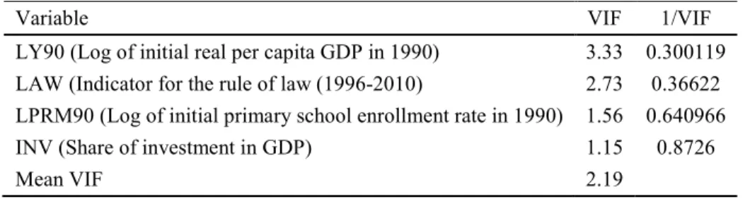
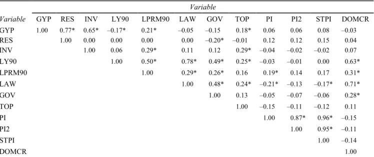
The second one is the multicollinearity problem or the strong correlation among all the right-hand-side variables. For example, investment, education, and a number of indicators used to measure the quality of government institutions in a country are all positively correlated with income per capita. It might be that one variable has a causal relationship with the other or that both variables, while not directly related, are caused by another variable. Multicollinearity reduces the precision with which coefficients are estimated: if two correlated variables are entered into a growth regression at the same time, the apparent strength of their individual relationship with growth might appear much weaker than if one or other is entered alone. However, multicollinearity does not bias the coefficients or the standard errors, which might explain why its effects seem less obvious for researchers.
Although they are important, international data are not only what growth discipline is about. Mankiw et al. (1995) provide a plausible explanation in this regard: “It is not that we have to stop asking so many questions about economic growth. We just have to stop expecting the international data to give us all the answers.”
1.3.2 Interpretation of coefficients
It is conceptually difficult to interpret the coefficients on regressions that involve data for over 100 countries averaged over 30 years during which time business cycles, policy changes,
and political instability have influenced economic activity. Therefore, the interpretation of these coefficients should be treated skeptically as many papers point to them as elasticities suggesting that if a policy indicator changes by one percent, growth will change by a percent corresponding to the coefficient on the policy indicator. However, partial correlation certainly does not imply causality. That is why cross-country regressions should be viewed as evaluating the strength of partial correlations and not as behavioral relationships that suggest how much growth will change following a change in policies (Levine and Renelt (1992); Levine and Zervos (1993a)).
1.3.3 National policies and growth
One goal of empirical work on economic growth is to establish the conditions that are associated with rapid growth. However, using cross-country analysis in order to examine national policies make things even more complicated as there is no clear proxies that measure policy actions. Cross-country regressions use policy indicators (e.g. the average ratio of exports to GDP or the average ratio of broad money to GDP over a time period) and do not typically link executable policies to growth. Several papers acknowledge the difficulty to find a measure or a proxy for variables that are fairly linked to the growth process (e.g. Levine and Zervos (1993a) and Kenny and Williams (2001)). Levine and Zervos (1993b) argue that it is “extremely difficult to identify believable links between a wide assortment of indicators of individual policies and long-run growth, although there is some evidence that general indicators of international distortions are negatively associated with growth.”5
One of the major difficulties is the multiplicity of possible regressors encountered by researchers trying to find empirical evidence on economic growth. There are logically unlimited possibilities of keys to growth, while the number of observations is clearly limited. Given that there is no easy solution to this degrees-of-freedom deficit, Kenny and Williams (2001) argue that this might reflect the fault of the econometric techniques used. One approach
5 In theoretical models of policy and growth, economists typically represent policy distortions with the Greek
is to move from cross-sectional to panel data as suggested by Barro and Sala-i-Martin (2004). Yet, there is no consensus on what the “right techniques” are.
1.3.4 Universalism:
Kenny and Williams (2001) specify two kinds of “universalism” that are inherent in cross-country growth regressions:
a) “Epistemological universalism”: the idea that all economic processes everywhere are, in principle, knowable—there is one basic production function driving all economies at all times and in every time-frame.
b) “Ontological universalism”: the view that economies share the same components and these components interact with one another in the same fashion.
Models of economic growth developed over the past 50 years are often in contradiction with one another. Thus, supporting that the process of economic growth works uniformly across countries through the statistical testing of variables in large cross-country regressions is likely to be inadequate, as argued by Kenny and Williams (2001). If multiple cross-country regressions over different samples, different time periods, and different econometric techniques suggest that a variable considered a determinant of growth is consistently and significantly related to growth rate, this provides support for the universality of the model. Kenny and Williams (2001) argue, however, that growth is a more complex process that can be captured by universal models and that economic growth thinking has often failed “to grasp the complex nature of the social world.”
All of these inherent obstacles to interpreting cross-country studies limit what economists can learn about policy-growth relationships. Kenny and Williams (2001) point out that “the evidence shows (…) that markedly different policies, and markedly different policy mixes, may be appropriate for different countries at difference times.”Levine and Zervos (1993a) argue that even if cross-country regressions yield very “strong” results, these results should be
viewed as “suggestive empirical regularities, neither as stylized facts nor as behavioral linkages relationships.” Mankiw et al. (1995) draw a more extremist conclusion: “Using these regressions to decide how to foster growth is (…) a hopeless task, (…) policymakers who want to promote growth would not go far wrong ignoring most of the vast literature reporting growth regressions.”
However, and despite these obstacles, cross-country regressions are very useful analytical tools for growth research as many economists believe that “its informational benefits override these objections,” as argued by Barro (1998). The main strength of the cross-country approach is that, as Barro (1998) argues, it shows the extent of experience needed for economists and policymakers to assess government policies and other determinants of economic growth in the long run. In fact, demonstrating that certain policy-growth linkages hold well across countries will influence beliefs about policy and economic performance.6 Equally, beliefs about policy and growth that are not supported by any cross-country evidence are likely to be viewed skeptically by policy advisers. In this context, Easterly (1995) suggests that “Policymakers should be convinced by looking at cross-country evidence that it is a lot better to make miracles feasible through good policy than to make them impossible by bad policy.” Finally, and in spite of the critics, the cross-country regressions technique have dominated the empirical literature of economic growth as many economists use it at a large scale.
Section 1.4 -
Sensitivity and Robustness
Kormendi and Meguire (1985) entered the explanatory variables independently and linearly, which will become a common feature of most cross-country growth regressions. Indeed, all potential variables cannot be included in one regression; simply, because the number of potential variables is larger than the number of countries in the world, rendering the all-inclusive regression computationally impossible (See the degrees-of-freedom problem discussed above). Instead, a typical empirical growth analysis considers only a small number
6
More attention has been paidin recent empirical literature to financial sector development indicators, which are obviously linked to changes in financial sector policies. Unfortunately, I do not test these variables because of lack of data.
of explanatory variables in attempt to establish a statistically significant relationship between growth and a particular variable of interest, to which the investigator point as an important determinant of growth. The analysis then proceeds to show that the variable of interest remains statistically significant when changes occur in the right-hand-side variables.
Economists typically prefer theoretically informed empirical investigations. Yet, it is hard to establish a consensus on the extent of trust one should put in the empirical findings as conditioning variables can have a significant impact on the apparent relationship between various factors in growth regressions. Economists have developed new methods in order to evaluate the robustness of these findings: Which variables are “truly” correlated with growth?
In attempt to provide an initial answer to this question and to put some order into the literature, Levine and Renelt (1992) assembled a cross-sectional data set with a large number of potential regressors and subjected it to a variant of Leamer’s (1983, 1985) extreme-bounds
analysis. Subsequently, Sala-i-Martin (1997a, b) points to Levine and Renelt’s (1992) method
as too strong and suggested his own, less restrictive variant on extreme-bounds analysis. I will discuss these two variants in details later on, but, first, I will summarize a few insightful ideas on the causes of the sensitivity of estimates in cross-country growth regressions.
If multiple cross-country regressions over different time periods, using different country sample and regression techniques show that a variable, considered significant in a growth model, is consistently and strongly related to growth, this may suggest the universal applicability of this model. Growth is, however, a more complex process than can be captured by universal models. As Kenny and Williams (2001) argue, the universal failure to produce robust causally secure relations predicted by models might suggest a broader problem than statistical methodological weaknesses. They specify two problems related to the theorizing about economic growth upon which econometric studies have been used:
a) Ahistoricism: There are probably virtuous and vicious cycles at work in development. The presence of these circles raises questions of long-term path dependency and so “historically-situated interpretations of the growth experience”. In some way, a small
difference in the initial conditioning sets of a country could send it off on very different growth trajectories.
b) Account of causality: Myrdal (1957) argues that not just economic growth may have a great number of causes, but also that these do not work in any linear manner. Economic growth should be examined using the concept of “circular causation”, where a change in one factor would affect other factors and these changes would in turn feedback on the first factor. However, different models generate different results. Levine and Zervos (1993a), for instance, argue that inflation has important negative effects on growth but only for very high levels of inflation. On the other hand, Barro and Sala-i-Martin (2004) find no evidence for such a suggestion.
In the 1990s, two main research methods were advanced by researchers to assess the sensitivity of estimates in cross-country growth regressions: i) The so-called Levine and Renelt’s (1992) modified version of Leamer’s extreme-bounds analysis (EBA) and ii) the Bayesian averaging method adopted by Sala-i-Martin (1997a, b).
1.4.1 Extreme-Bounds Analysis:
The central idea of Leamer’s analysis is that a coefficient of interest is robust only to the degree that it displays a small variation to the presence or absence of other regressors. A variable is said to be robust if its extreme bounds lie strictly to one side or the other of zero. And the narrower the extreme bounds, the more confidence one is supposed to have in the coefficient estimate.
In their paper A Sensitivity Analysis of Cross-Country Growth Regressions, Levine and Renelt (1992) conducted one of the very first comprehensive reviews of the empirical growth literature—at the time—according to which over 50 variables were found to be significantly correlated with long-term growth in at least one regression. They extended the types of exploratory cross-country empirical investigations of growth developed by Kormendi and Meguire (1985) and advanced by Barro (1991a, b) Although these two studies presents “appealing results each”, Levine and Renelt (1992) show that a union of the two sets of
explanatory variables leaves none of the economic policy indicators significantly correlated with growth.
Levine and Renelt (1992) examine the relationship between economic growth and a wide assortment of fiscal expenditure, fiscal revenue, monetary, trade, and political indicators for a broad cross-section of countries over the 1960-89 and 1974-89 periods.7 They apply a modified version of Leamer (1983, 1985) extreme-bounds analysis (EBA) to identify the robustness of empirical relations for economic growth. A variable is pointed to as “robust” if its estimate keeps the same theoretical sign and significant correlation with the dependent variable in all regressions with different conditioning sets.8 Otherwise, the test would label it as “fragile”. A practical problem in implementing extreme-bounds analysis is the large number of potential regressors. Levine and Renelt (1992) simplify the problem by adopting Leamer’s notion that some variables should be included in every single regression (on the assumption that they are known to be robust a priori9). Finally, they consider regressions with no fewer than five and no more than eight independent variables.
The main result in the Levine and Renelt (1992) analysis is that cross-country regressions’ findings are fragile to small alterations in the conditioning information set. In fact, they find none of the wide assortment of fiscal-expenditure variables, international trade and distortion measures, monetary-policy indicators, and political-stability indices considered by the profession to robustly correlate with growth, except for the index of coups and revolutions.10
Levine and Zervos (1993a) slightly modify the approach taken in Levine and Renelt (1992). They test indicators of the level of domestic financial sector development, an
7
Their original data set contains 40 variables for 119 countries. Reporting is not complete so that the 199 x 40 matrix of variables has many missing values.
8
Z-variables average rate of government consumption expenditure to GDP, the ratio of exports to GDP, the average inflation rate, the average growth rate of domestic credit, the standard deviation of domestic credit growth, and an index for the number of revolutions and coups.
9
They chose the variables that are always included in the regression based on past empirical studies and economic theory. These variables are the following: the investment share of GDP, the initial level of real GDP per capita in 1960 from the Summers-Heston data set(SH), the initial secondary-school enrollment rate, and the average annual rate of population growth.(Levine, Ross and David Renelt. 1992. "A Sensitivity Analysis of Cross-Country Growth Regressions." The American Economic Review, 82(4), 942-63.)
10 Robust partial correlations were found between growth and the following I-variables: the ratio of investment,
improved measure of the black market exchange rate premium, a measure of the total public sector surplus, and use a reduced set of permanent variables or what is frequently called “Barro regressors”: the log of the initial secondary school enrollment rate, the log of the initial real GDP per capita, and an index for the number of revolutions and coups.
Levine and Zervos (1993a) find various indicators of financial sector development robustly associated with long-term growth. This result may suggest that the relationship between financial sector policies and long-run growth deserves more empirical investigation. Moreover, they identify the black market premium to be negatively related to growth in the Barro-style regression framework. Finally, as in Levine and Renelt (1992), a host of monetary, fiscal and trade indicators are not robustly related to growth. Levine and Renelt (1992) and Levine and Zervos (1993a, b) argue that it is extremely difficult to identify reliable statistical relationship between a broad assortment of indicators of individual policies and long-run growth.11
Mankiw et al. (1995) argue that the sensitivity of estimates to specification of the right-hand-side variables included in the regression is a result of the multicollinearity problem. Levine and Renelt (1992) themselves argue that one possible objection to this EBA is that it introduces multicollinearity, inflates the coefficient standard errors, and exaggerates the range on the coefficient of interest. However, as Leamer (1983) points out that “The collinearity in naturally selected treatment variables may mean that the data evidence is weak, but it does not invalidate in any way the usual least squares estimates.”
Several papers reproach the EBA search process for being pessimistic. Indeed, in order to be labeled as robust, a variable must enter significantly and with the sign suggested by theory in all regressions. This led Barro and Sala-i-Martin (2004) to criticize the test for allowing every single regression to hold a “veto power” to render a variable non-robust. Hoover and Perez (2004) criticize this method for being misleading about the determinants of growth as it
11
The pool of Z-variables includes the average inflation rate, the standard deviation of inflation, the government fiscal surplus ratio to GDP, imports plus exports as a share of GDP, the black market premium, and liquid liabilities as a ratio of GDP, for a total of seven possible Z variables.
rejects too many potential sources of growth for not being robust. However, Levine and Renelt (1992) point out clearly that their aim is not to identify causes of growth.
Another consideration is the exogeneity of right-hand-side variables. Sala-i-Martin (1997a, b) and Hoover and Perez (2004) observe that Levine and Renelt’s (1992) data set includes variables that are endogenous as potential regressors.
On the other hand, Kenny and Williams (2001) reproach the EBA test for being “excessively restrictive” as it excludes some factors that indirectly do have an impact on growth by excluding variables that are only correlated with growth because they are caused by another factor that itself has a causal relationship with growth.12 In the same context, Hoover and Perez (2004) suggest that robustness in Leamer’s fashion is an inadequate guide to model specification (whatever other uses it might have). They argue that there is no reason to suppose that omitting variables from search universe makes EBA any more informative than when they are included. They also consider that extreme-bounds approaches in the form advocated by Levine and Renelt (1992) “are too stringent and reject truth too frequently”.
Finally, Kenny and Williams (2001) criticize the EBA analysis because it measures the robustness of correlation, but says little about causation between variables. They argue that conditioning variables can have a significant impact on the apparent relationship between factors in growth regressions. I should point out that correlation, however, does not prove causation and even finding a robust partial correlation does not imply that this variable of interest causes growth. Moreover, Levine and Renelt (1992) indicate that their results do not depend importantly on choosing these variables.
Nevertheless, Levine and Zervos (1993a) suggest that the main contribution of Levine and Renelt’s (1992) work is showing that past findings typically rely on searching beyond standard regression specifications to find the “right” set of right-hand-side variables that produce “good” results. In addition, the methodological utility of extreme-bounds analysis is quite valuable as a means of communicating model uncertainty.
12
They argue that, in other ways, this test is not restrictive enough as it is only performed on a one-period global sample.(Kenny, Charles and David Williams. 2001. "What Do We Know About Economic Growth? Or, Why Don't We Know Very Much?" World Development, 29(1), 1-22.)
Sala-i-Martin (1997a, b) argues that this test was “too strong for any variable to pass it”. He moves away from extreme tests and assign some level of confidence to each of the variables.
1.4.2 Bayesian Averaging of Estimates:
Sala-i-Martin’s (1997a, b) averaging of estimates across models approach modifies the EBA procedure in two ways. First, at the equation level, he considers only regressions of exactly seven regressors, including (exactly) three variables from the pool of policy indicators. He tries every single linear combination of these three variables in the search universe. Second, he adopted a new criterion for robustness. The estimate of a coefficient on a focus variable is robust if 95% or more of the estimates (±2 SEs) lie to one or other side of zero.
In order to assign a level of confidence to each variable, Sala-i-Martin (1997a, b) constructs weighted averages of all estimates on the variables of interest and their corresponding standard deviation using “weights proportional to the likelihoods of each of the models.” In this context, Barro and Sala-i-Martin (2004) argue that a natural way to think about model uncertainty is to admit that we ignore which model is “true” and, instead, attach probabilities to different possible models. Furthermore, to account for Levine and Renelt (1992) endogeneity problem in a new data set, to a greater degree, Sala-i-Martin (1997a, b) collected variables that were likely to be predetermined, so that a causal reading of their relationship to the rate of growth per capita GDP is more plausible.
Sala-i-Martin (1997a, b) suggest that if most of the correlations are of the same sign even allowing for different conditioning sets, then the variable has a strong relationship with growth and should be regarded as robust.13 He obviously finds more variables to have robust relationships with growth, as compared to Levine and Renelt (1992). In his four-million regression test paper, 21 variables survive the process. However, I should point out that fully half of these variables can be considered “structural” and only two can be viewed as policy variables (degree of capitalism and number of years an open economy).
13 One finding is that all variables are insignificant for a subset of the models. Hence, the Levine and Renelt
Fernandez et al. (2004) criticize this method for not being Bayesian. Sala-i-Martin et al. (2004) propose an enhanced method, Bayesian Averaging of Classical Estimates (BACE), which combines the averaging of estimates across models with classical ordinary least squares (OLS) estimation. They apply BACE to a set of 67 variables selected according to two criteria. First, they use variables that are available as closely as possible to the beginning of the sample, 1960. Second, they use variables that allow for a balanced data set; that is, an equal number of observations for all regressions.
This test allocates the variables into three categories: variables strongly related to growth, marginally related to growth, and not robustly related to growth.14 Among the 18 variables that are strongly related to growth rate, the top variable is the dummy for East Asian countries, which is positively related with economic growth. The finding, of course, reflects the exceptional economic performance of these countries between 1960 and the mid-1990s. Measures of human capital are found (positively) strongly related to growth (e.g. Primary schooling in 1960 comes second and Malaria prevalence in 1960s seventh). There is statistical evidence for conditional convergence (Log of GDP in 1960 is ranked fourth). Some other geographical, historic, and cultural variables appear in this category as well.15
On the shortcomings of this approach, one can argue that there is missing information. Some interesting variables in the literature are excluded from the analysis as well as countries. Moreover, Barro and Sala-i-Martin (2004) observe that the statistical properties of weighted averages are not derived from a statistical theory and this is the reason why they are unlikely to be well understood. Kenny and Williams (2001) point out that the variables used are only shown to be weakly robust in a one period regression using a largely constant set of countries.
14
To establish these ranks, they report the posterior inclusion probability of a variable in the growth regression. Thus variables with high inclusion probabilities are the ones that have high marginal contribution to the goodness of the regression model. Then, they test whether the data increase or decrease the inclusion probability relative to the prior probability. Variables strongly related to growth are those with increasing posterior inclusion probability to the prior probability after having estimated all the regressions. See Sala-i-Martin, Xavier; Gernot Doppelhofer and Ronald I. Miller. 2004. "Determinants of Long-Term Growth: A Bayesian Averaging of Classical Estimates (Bace) Approach." The American Economic Review, 94(4), 813-35.
15Interestingly, some macroeconomic variables, such as the inflation rate, do not appear to be strongly related
Hoover and Perez (2004) criticize the approach advocated by Sala-i-Martin (1997a, b) for being “not discriminating and accept the false too frequently along with the true.” They argue that differences in growth rates across countries are more adequately characterized by a much smaller number of variables and suggest a “general-to-specific” method which they believe correspond reasonably well to a priori growth theory and to a reasonable understanding of political and cultural factors. Their search process, however, fails to select real per capita GDP in 1960 or any human-capital-related variables (e.g. primary school enrollment or life expectancy).
Having discussed the most important contributions to the literature on economic growth, I know move to present the model and the results of this paper.
Chapter 2 - Model and Results
“There does not exist a consensus theoretical framework to guide empirical work growth, and existing models do not completely specify the variables that should be held constant while conducting statistical inference on the relationship between growth and the variables of primary interest.”16 Economists can use Leamer’s work on extreme-bounds analysis (EBA) to evaluate the “believability” of cross-country regressions. Indeed, EBA represent one, very limited, measure of this believability.
Section 2.1 -
Methodology and Model
I briefly explain the EBA of Leamer. Assume a pool of Ω variables that previously have been identified to be related to growth and one is interested in knowing whether a variable M is robust—i.e., the corresponding coefficient remains significant and of the same sign at the extreme bounds following various alterations in the conditioning information set. One would estimate regression that employs the linear ordinary least squares (OLS) regression framework:
(1) Y = βij I + βmj M + βzj Z + µj
where I is a vector of variables that always appear in the regressions, M is the variable of interest, and Z is a vector of variables, taken from the pool of the Ω variables available, that one believes it represents an appropriate conditioning information. For each model j, one finds an estimate, βmj, and the corresponding standard deviation, σmj, computes the extreme upper
and lower bounds on the coefficient βmj. The extreme upper bound is equal to the highest
calculated value of βm + 2 σm, while the extreme lower bound is defined to be lowest value of
βm – 2 σm. These extreme bounds can help clarify the degree of confidence we can place in the
partial correlation between growth and the variable of interest.
16
Levine, Ross and David Renelt. 1992. "A Sensitivity Analysis of Cross-Country Growth Regressions." The
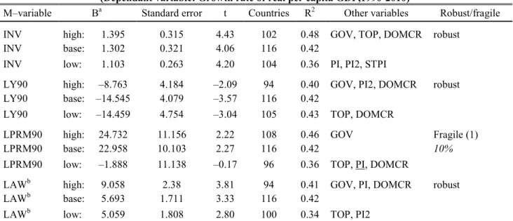
As regards this paper, the dependent variable Y is the average annual growth rate of real GDP per capita over the 1990-2010 period. First, for each variable of interest, M, I run a baseline regression with only the basic set of variables. This base regression determines whether the variable of interest is significantly correlated with long-term growth after controlling for a base set of variables. The baseline estimation results with a prior expected model size of 5 variables—that is, I-variables along with the variable of interest.
Second, I restrict the number of subsets of Z-variables by considering only subsets with three or fewer variables. I run separate regressions including each variable—one at a time— from the pool of potential Z variables; then regressions including every combination of two Z-variables; finally, regressions including every combination of three Z-variables. Consequently, the largest regression has 8 explanatory variables: that is, four I-variables, 1, 2 or 3 Z-variables, and the variable of interest (M). Although the model size is in some sense arbitrary, I believe it is reasonable and motivated by the fact that most empirical growth studies include a moderate number of explanatory variables, as argued by Barro and Sala-i-Martin (2004, p. 552).
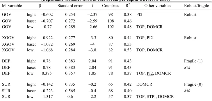
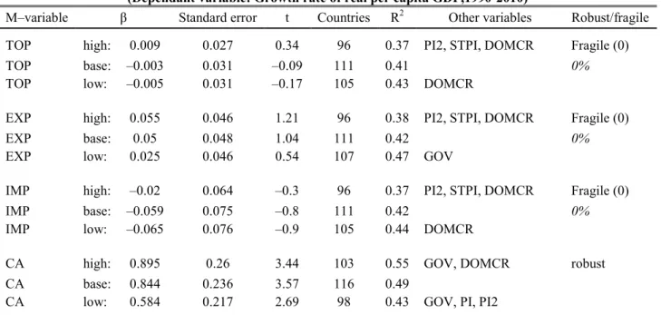
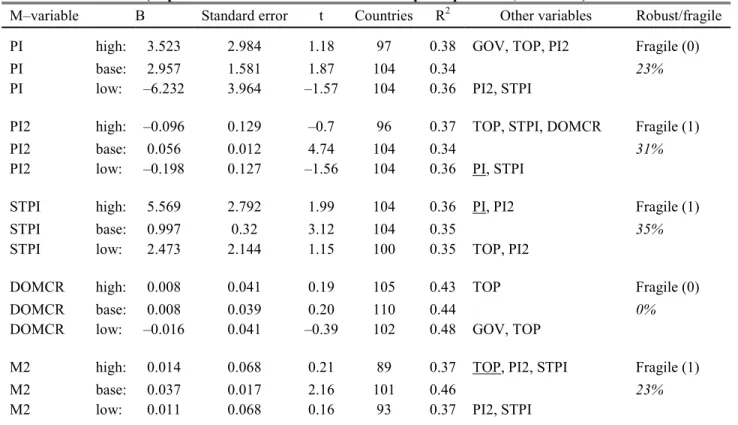
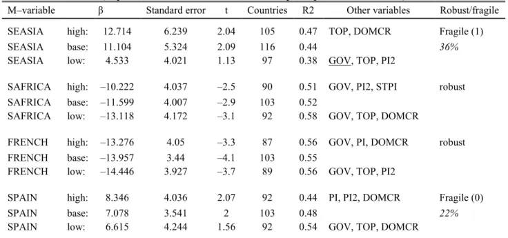
Like in a standard EBA test, if the coefficient on the variable of interest remains significant and of the same theoretical sign at the extreme bounds, I will report it as robust, if not as fragile. A coefficient is significant if it cannot be rejected at the standard level of significance P = 0.05. If a result is fragile, the results tables will also indicate the number of variables needed to be added before the variable of interest is insignificant or of the wrong sign, in addition to the percentage of time the M-variable’s extreme bounds are of the same sign. Of course, finding a robust partial correlation does not necessarily imply that the variable of interest causes growth.
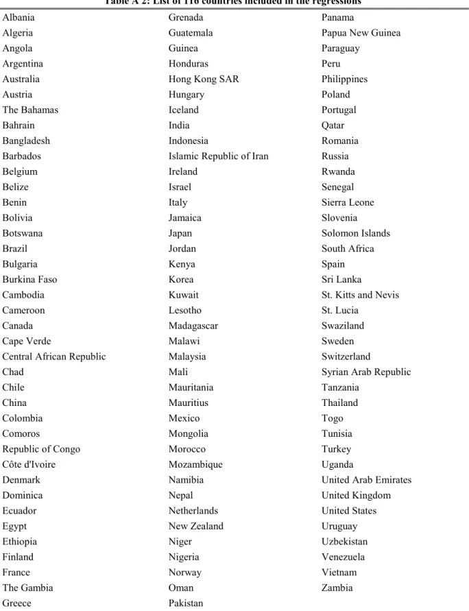
I replicate the test of Levine and Renelt (1992). I use different sets of variables for a broad cross-section of 116 countries (see the country list).17 I use more recent data related to the 1990-2010 period. The choice of the sample period was motivated by several reasons. First, I
17I should point out that neither former Soviet Republics nor socialist East European countries are included in
want to test whether looking at different period would necessarily imply different sensitivity results. Second, the starting year (1990) is a turning point for the global economic system following the German reunification. Third, I did not extend other historical data sets, e.g. Levine and Renelt (1992), Barro and Lee (1993, 2010) or Sala-i-Martin (1997b), that cover data before 1990 for consistency purposes and because of the lack of information on some variables.18 Finally, as I discussed earlier, it is conceptually difficult to interpret the results for a large sample of country over a very long period of time. Similarly to the work of Levine and Renelt (1992), I obtained most data from the World Bank and the International Monetary Fund’s databanks, the initial income figures from Heston et al. (2012), hereafter SH, and the geographical dummy variables from Sala-i-Martin (1997a, b).
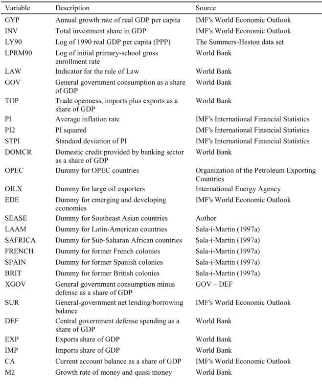
All variables are averaged over the 1990-2010 period19.Compiling a complete data matrix with no missing values is difficult. At the variable level, I omit countries for which data are missing for 3 years or more during the study period. However, I believe that any error left due to this omission is relatively small in the aggregate. I used and compiled over 20 variables (an exhaustive list of variables used appears in annex). At the aggregate level, and in accord with Levine and Renelt (1992) and Sala-i-Martin (1997a, b), I deal with the missing data problem through the so-called casewise (or listwise) deletion. Hoover and Perez (2004) describe this method as follows: “for any regression, if a country does not report the values for each of the variables required for that regression, that country is omitted from the regression.”20 Furthermore, I use variables measured as closely as possible to the beginning of the sample period (i.e. 1990). This is partly done to deal with the endogeneity problem, as argued by Sala-i-Martin, et al. (2004). Variable units are either percentage change or ratios for comparability purposes. With these restrictions, the total size of the data set becomes 26 variables (including the dependant variable, the annual growth rate of GDP per capita between 1990 and 2010) for
18
According to the IMF’s WEO database it is difficult to verify the accuracy of historical data before 1980.
19
Except for the rule of law indicator (LAW), that is averaged over the 1996-2010 period.
20They opt for the multiple imputation method instead. They argue that the casewise deletion presents two
particular problems. First, it wastes enormous amounts of relevant information. They questioned the legitimacy of comparing coefficient estimates across millions of EBZ regressions conduced on different country samples (Hoover, Kevin D. and Stephen J. Perez. 2004. "Truth and Robustness in Cross-Country Growth Regressions*."