An iterative two-step heuristic for the parallel drone scheduling traveling salesman problem

HAL Id: hal-01952007

https://hal.archives-ouvertes.fr/hal-01952007

HAL is a multi-disciplinary open access

archive for the deposit and dissemination of sci-entific research documents, whether they are pub-lished or not. The documents may come from teaching and research institutions in France or abroad, or from public or private research centers.

L’archive ouverte pluridisciplinaire HAL, est destinée au dépôt et à la diffusion de documents scientifiques de niveau recherche, publiés ou non, émanant des établissements d’enseignement et de recherche français ou étrangers, des laboratoires publics ou privés.

scheduling traveling salesman problem

Raïssa Mbiadou Saleu, Laurent Deroussi, Nathalie Grangeon, Alain Quilliot,

Dominique Feillet

To cite this version:

Raïssa Mbiadou Saleu, Laurent Deroussi, Nathalie Grangeon, Alain Quilliot, Dominique Feillet. An iterative two-step heuristic for the parallel drone scheduling traveling salesman problem. Networks, Wiley, 2018, 72 (4), pp.459-474. �10.1002/net.21846�. �hal-01952007�

An iterative two-step heuristic for the

Parallel Drone Scheduling Traveling

Salesman Problem

Raïssa G. Mbiadou

Saleu

Université Clermont Auvergne LIMOS UMR CNRS 6158, 63178

Aubière Cedex, France raissa.saleu@isima.fr

Laurent Deroussi

Aubière Cedex, France laurent.deroussi@uca.fr

Dominique Feillet

feillet@emse.fr

Nathalie Grangeon

Université Clermont Auvergne LIMOS UMR CNRS 6158, 63178

Aubière Cedex, France nathalie.grangeon@uca.fr

Alain Quilliot

Aubière Cedex, France alain.quilliot@isima.fr

ABSTRACT

Delivery of goods into urban areas constitutes an important issue for logistics service providers. One recent evolution in urban logistics involves the usage of drones in the delivery process. Delivery by drones offers new possibilities, but also induces new challenging routing problems. In this paper, we address a heuristic solution of the so-called Parallel Drone Scheduling Traveling Salesman Problem, recently introduced by Murray and Chu [19]. In this problem, deliveries are split between a vehicle and one or several drones. The vehicle performs a classical delivery tour from the depot, while the drones are constrained to perform back and forth trips. The objective is to minimize the completion time. We propose to solve the problem with an original iterative two-step heuristic, composed of: a coding step that transforms a solution into a customer sequence, and a decoding step that decomposes the customer sequence into a tour for the vehicle and series of trips for the drone(s). Decoding is expressed as a bicriteria shortest path problem and is carried out by dynamic programming. Experiments conducted on benchmark instances from the literature confirm the efficiency of the approach and give some insights on this drone delivery system.

KEYWORDS

1

INTRODUCTION

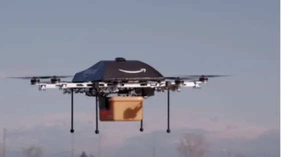
Last mile logistics has become a popular area of interest for retailers. Companies are always searching for fast and cost-efficient ways to deliver goods to their customers. It is from this perspective that in 2013, the chief executive officer of the largest online retailer Amazon revealed a revolutionary project of the company called Prime Air [1], a drone designed to deliver packages in just 30 minutes (Fig. 1). In August 2014, Google followed by revealing its drone delivery project called wing, with experiments run in Australia. In September 2014, DHL Express launched its parcelcopter, a helicopter-style drone which could deliver medications and urgently needed goods to the remote North Sea island of Juist [2]. In 2015, the online retailer Alibaba tested the usage of drones to deliver online orders of tea to customers in China [16]. In April 2016, Autralia post started testing the usage of remotely piloted drones internally for parcel delivery, with the support of the Civil Aviation Safety Authority [3]. In July 2016, convenience store chain 7-eleven made their first commercial delivery with drone, partnered with the drone start-up Flirtey[17]. United Parcel Service (UPS) company is testing drones to deliver medicine to an island near Boston [20]. Still in july 2016, the first humanitarian drone called Zipline arrived in Rwanda. Zipline is a drone of about 10 kilos that is capable of carrying 1.3 kilos of medicines or blood [4]. In August 2016, Domino’s Pizza announced their intention to extend to France their experiments on pizza delivery by drone, as initiated in New Zealand [5]. Many other companies not mentioned above have launched similar projects.

Previously exclusively used in military applications, drones are becoming a part of the last mile delivery concept which can significantly accelerate delivery times and reduce human intervention. Indeed, drones are lightweight, they consume less energy than standard vehicles and they are not subject to congestion problems since they do not follow the road network. On the other hand, drones are limited in terms of endurance, capacity and payload. Despite several regulatory and safety standards barriers, the idea of using Unmanned Aerial Vehicle (UAV) for parcel delivery is gaining ground. Companies that want to use drones in their delivery process are confronted by air control administrations like the FAA1_{in the United States or the DGAC}2_{in France. The scientific community is} getting more and more interested in investigating the design of drone delivery systems.

In this paper, we are interested in the development of efficient solution methods for a specific drone delivery system. The remainder of the paper is organized as follows. In Section 2, we present the related literature. In Section 3, we formally describe the problem addressed in this paper and provide an integer linear programming formulation. We propose a heuristic to solve the problem in Section 4. In Section 5, we discuss the results obtained from our computational experiments. Finally, we conclude with some directions for future researches in Section 6.

Figure 1 Amazon Prime Air (source: amazon.com)

1_{Federal Aviation Administration} 2_{Direction Générale de l’Aviation Civile}

2

RELATED WORK

The problem of parcel delivery with drone has received increasing attention these last years. Murray and Chu [19] introduced the Flying Sidekick Traveling Salesman Problem (FSTSP) and the Parallel Drone Scheduling Traveling Salesman Problem (PDSTSP). In both problems, the optimization criterion is the minimization of the completion time, i.e., the time elapsed between the beginning and the end of the delivery process.

In the FSTSP, deliveries are performed by a single vehicle and a single drone working in tandem. The vehicle carries the drone and when the vehicle is at a customer location, it can decide to launch the drone to visit another customer location. After this drone delivery, the vehicle will then have to retrieve the drone at another customer location. Formally, a drone trip is represented as a triplet < i, j,k > where i is the launching point, j is the service point and k is the rendez-vous point (i , j, j , k and i , k). Figure 2 shows an illustration of the synchronization mechanism in the FSTSP. The authors proposed a Mixed-Integer Linear Programming (MILP) formulation and a heuristic that first constructs a TSP tour visiting all the customer locations and next, repeatedly run a relocation procedure to assign some customer requests to the drone.

Figure 2 FSTSP: Illustration of the synchronization mechanism (source [19])

The second problem introduced by Murray and Chu [19], the PDSTSP, simplifies the FSTSP setting by relaxing the synchronization issue between the vehicle and the drone. Conversely, it considers a fleet of drones instead of a single drone. The vehicle visits a subset of customers with a TSP tour and the drones serve the remaining customers directly from the depot with back and forth trips. Again, the authors proposed a MILP formulation and a heuristic. The principle of the heuristic is to partition the set of customers into two subsets (a vehicle set and a drone set). Then, a TSP tour is computed for the customers assigned to the vehicle and a Parallel Machine Scheduling (PMS) problem is solved to assign customer requests (jobs) to drones (machines). At the end, an improvement step is performed to reassign customers either to the drone set or to the vehicle set in order to better balance vehicle and drones activities.

In his Master Thesis, Ponza [21] addresses the FSTSP and proposes a simulated annealing heuristic.

Wang et al. [23] studied an extension of the FSTSP called the Vehicle Routing Problem with Drones (VRPD) in which they considered a homogeneous fleet of trucks, each one of them carrying several identical drones. A drone launched from a truck must be picked up by the same truck at the same or at a different location. The objective is still to minimize the completion time. The authors proposed worst-case analyses and obtained theoretical bounds on the benefits achieved using drones.

In [6], Agatz et al. introduced another variant of the FSTSP that they called the Traveling Salesman Problem with Drone (TSP-D). Contrary to the FSTSP, the launching point of a drone and the rendezvous point with the vehicle are not necessarily different. Furthermore, the objective is to find the shortest tour to serve all customer locations either by the vehicle or the drone. The authors proposed an Integer Programming (IP) formulation and a route first -cluster secondheuristic.

Ha et al. [12] adopted the name TSP-D for the FSTSP. They proposed a cluster first - route second and a route first - cluster secondheuristic. In [13], the same authors investigated a different objective function: the minimization of the total transportation cost for both the vehicle and the drone. They coined this problem as min-cost TSP-D. They proposed a MILP model and two heuristics: one based on a Greedy Randomized Adaptive Search Procedure (GRASP) and another one called TSP-LS adapted from the work of Murray and Chu [19].

Dorling et al. [8] introduced a very different problem that they called Drone Delivery Problem (DDP). They considered two variants of the DDP: the Minimum Cost Drone Delivery Problem (MC-DDP) that aims at minimizing the total delivery cost and the Minimum Time Drone Delivery Problem (MT-DDP) that aims at minimizing the total delivery time. In these problems, deliveries are only performed by drones, and the energy consumption is explicitly considered for the drones, taking into account their payload. The authors established the relationship with the Multi-Trip Vehicle Routing Problem (MTVRP). They proposed a MILP formulation and a Simulated Annealing (SA) heuristic.

Ulmer and Thomas [22] studied a dynamic variant of the PDSTSP. They called their problem Same-Day Delivery Routing Problem with Heterogeneous Fleets (SDDPHF). The SDDPHF considers two fleets of vehicles and drones that deliver goods from the depot to customers who dynamically request services. When a new customer request arrives, a dispatcher has to decide whether or not to accept the customer for the same-day delivery and determine the according assignment and routing decisions. The SDDPHF takes into account a time window for each request, the loading time for both vehicles and drones, the time to drop off a package from a vehicle or a drone as well as the recharging or battery swap time for drones. The objective is to maximize the expected number of customers served the same day. To solve the problem, the authors proposed an adaptive dynamic programming approach called parametric policy function approximation (PFA).

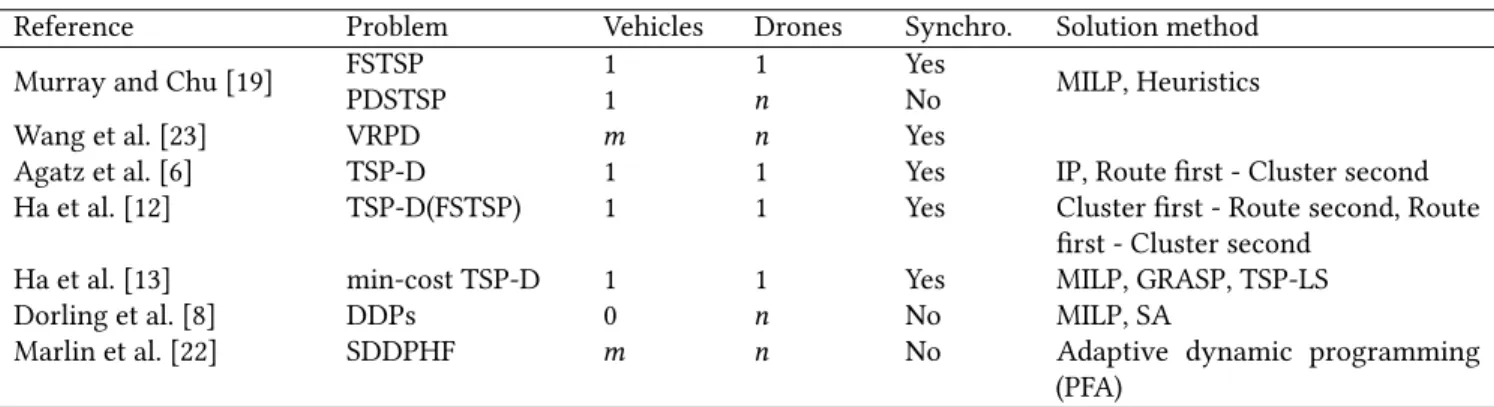
Table 1 gives a summary of the main papers on drone delivery problems found in the literature.

In connection with the literature on drone delivery, we can also mention the Carrier-Vehicle TSP, addressed by Garonne et al. [10] or Gambella et al. [9]. In this problem, two vehicles with different capabilities cooperate. The carrier is slow but has a virtually infinite operating range. Its role is to deploy and recover a second vehicle, typically an aircraft, which is faster but has a reduced operating range.

3

THE PARALLEL DRONE SCHEDULING TRAVELING SALESMAN

PROBLEM

In this paper, we focus on the PDSTSP, presented in [19], that we found more relevant on a short term in view of actual delivery practices and that has yet drawn less attention in the literature. The PDSTSP is formally defined below.

Reference Problem Vehicles Drones Synchro. Solution method Murray and Chu [19] FSTSP_PDSTSP 1_{1 n}1 Yes_No MILP, Heuristics Wang et al. [23] VRPD m n Yes

Agatz et al. [6] TSP-D 1 1 Yes IP, Route first - Cluster second Ha et al. [12] TSP-D(FSTSP) 1 1 Yes Cluster first - Route second, Route

first - Cluster second Ha et al. [13] min-cost TSP-D 1 1 Yes MILP, GRASP, TSP-LS Dorling et al. [8] DDPs 0 n No MILP, SA

Marlin et al. [22] SDDPHF m n No Adaptive dynamic programming (PFA)

Table 1 Optimization of drone delivery systems

3.1

Problem definition and notation

We consider a complete directed graph G = (N ∪ {0}, A) where N = {1, . . . ,n} is a customer set and 0 is the depot. A vehicle and a fleet of M drones are available to deliver parcels to customers. The vehicle delivers customers with a single tour starting from the depot, visiting a subset of customers and returning back to the depot. Drones operate back and forth trips between the depot and the customers, delivering a single customer in each trip. Not all customers are eligible for drone delivery, because of practical constraints such as the limited payload or the flying range of drones. The subset of customers that can be served by a drone is denoted Nd. These customers are consistently called drone-eligible in the rest of the paper. Figure 3 depicts a solution of the PDSTSP on an instance with 10 customers, among which 5 are drone-eligible.

depot 1 2 3 4 5 6 7 8 9 10 vehicle drone 1 drone 2 Not drone-eligible Drone-eligible Legend:

Figure 3 A set of 10 customers served by 1 vehicle and 2 drones.

A travel time dijis incurred when the vehicle goes through an arc (i, j) ∈ A. A travel time bdi is incurred when a drone serves a customer i ∈ Nd. Assuming that both the vehicle and the drones can start from the depot at time 0,

the objective of the PDSTSP is to minimize the delivery completion time, i.e., the time at which the vehicle and all drones are back to the depot, with the service of all customers carried out.

3.2

MILP formulation

In this section, we express the PDSTSP with a MILP formulation. We introduce the following binary decision variables :

• zi = 1 if customer i is visited by the vehicle, 0 if it is visited by the drone (i ∈ N ); • x_ij = 1 if arc (i, j) belongs to the vehicle tour, 0 otherwise ((i, j) ∈ A);

• yim= 1 if customer i is assigned to drone m, 0 otherwise (i ∈ Nd, 1 ≤ m ≤ M). In addition, we introduce a nonnegative variable T that represents the completion time.

The model is:

minimize T (1) subject to T ≥ Õ (i, j)∈A dijxij (2) T ≥ Õ i ∈Nd b diyim (1 ≤ m ≤ M) (3) zi = 1 (i ∈ N \ Nd) (4) Õ (i, j)∈A xij = zi (i ∈ N ) (5) Õ 1≤m ≤M yim = 1 − zi (i ∈ Nd) (6) Õ (0, j)∈A x_0j ≤ 1 (7) Õ (i, j)∈A xij = Õ (k,i)∈A xki (i ∈ N ) (8) Õ i ∈S Õ j<S xij ≥Õ i ∈S zi+ 1 − |S| (S ⊆ N , S , ∅) (9) zi ∈ {0, 1} (i ∈ N ) (10) xij ∈ {0, 1} ((i, j) ∈ A) (11) yim ∈ {0, 1} (i ∈ Nd, 1 ≤ m ≤ M) (12) T ≥ 0 (13)

The objective (1) is to minimize the completion time T . Constraints (2) and (3) give lower bounds on T expressed using vehicle assignment and drone assignment variables. Constraints (4) ensure that all the customers that are not drone-eligible are served by the vehicle. Constraints (5) and (6) guarantee that every customer is served either by the vehicle or a drone, exactly once. Constraint (7) stipulates that the vehicle leaves the depot at most once. Constraints (8) ensure flow conservation for the vehicle tour. Subtour elimination constraints are provided by (9). These constraints ensure that given a non empty subset of customers S ⊆ N , if all the customers in S are visited by the vehicle, there is at least one outgoing arc from S. Finally, constraints (10) to (13) define the decision variables.

4

ITERATIVE TWO-STEP HEURISTIC

The PDSTSP can be considered as a bilevel problem in which:

• at the first level, customers are partitioned between the vehicle and the fleet of drones;

• the second level manages the routing optimization, which consists in solving two NP-Hard problems, namely: a TSP for the vehicle and a Parallel Machine Scheduling (PMS) problem for drones.

Our iterative two-step heuristic alternates between these two levels. Given a solution of the PDSTSP, a coding step transforms this solution into a customer sequence. Then, a decoding step decomposes this sequence into a tour for the vehicle and series of trips for the drones. These tours / trips are optimized and the process is repeated. The general solution framework does not depend on the number of drones, but the decoding procedure does. When M = 1, i.e., a single drone is available, the decoding scheme is exact. When M > 1, it is heuristically extended.

In Section 4.1, we describe the general scheme of the heuristic. The decoding procedure is detailed in Section 4.2 when M = 1. We explain how it is adapted to M > 1 in Section 4.3. In these sections, we adopt the following notation. A solution S is represented as a vector of M + 1 customer sequences (τvehicle, τ1, . . . , τM), where τvehicle indicates the visit order of the customers for the vehicle and τ1to τM this order for the M drones. We denote c1(S) the completion time for the vehicle in solution S and c2_{(S) the completion time for the fleet of drones. Finally,} c(S) = max(c1_{(S), c}2_{(S)) is the solution cost.}

4.1

General scheme of the iterative two-step heuristic

The general scheme of our heuristic is summarized in Algorithm 1 and is explained hereafter. Algorithm 1General scheme of the iterative two-step heuristic

1: τ ← solveTSP() 2: bestSol ← (τ , ∅, . . . , ∅)

3: whilebestSol is improved do

4: (τvehicle, τdrones) ←split(τ )

5: τ_vehicleopt ←reoptimizeTSP(τ_vehicle)

6: (τ₁opt, . . . , τ_Mopt) ←optimizePMS(τ_drones)

7: ifsolution (τ_vehicleopt , τ₁opt, . . . , τ_Mopt)is better than bestSol then

8: bestSol ← (τ_vehicleopt , τ₁opt, . . . , τ_Mopt)

9: τ ← bestInsertion(τ_vehicleopt , τ₁opt, . . . , τ_Mopt)

10: end if

11: end while

In lines 1 and 2, we build a giant TSP tour τ visiting the depot and all the customers. For that matter, we apply a nearest-neighbor construction procedure. The TSP tour provides a starting solution (τ, ∅, . . . , ∅) for our algorithm, where all the customers are visited by the vehicle in the order of sequence τ and no customer is assigned to the drones.

The main part of the algorithm is given by lines 4 to 9 that are repeated as long as they enable finding better solutions. A solution S is considered to be better than another solution S′_{if one of the two following conditions} hold:

• c(S) < c(S′)

Decoding procedure split on Line 4 decomposes τ in two complementary subsequences: one assigned to the vehicle (τvehicle) and one assigned to the fleet of drones (τdrones). This procedure, which is central in the algorithm, is detailed

below. Vehicle route τvehicle is then reoptimized, with Helsgaun’s implementation of Lin-Kernighan heuristic [14]

(Line 5) and a PMS solution is obtained from τdrones (see Section 4.3). The new solution (τ_vehicleopt , τ₁opt, . . . , τ_Mopt)is

compared with bestSol and the latter is updated if needed. Finally, in this case, all the customers from τ₁opt, . . . , τ_Mopt are reinserted in τ_vehicleopt , in this order and with a best insertion policy (Line 9). Otherwise the algorithm stops.

Note that when M = 1, the PMS problem is trivial, hence one can replace Line 6 with τ₁opt ←τ_drones.

4.2

Decoding procedure when

M = 1

We first consider the case M = 1. Procedure split(τ ) computes the best partition of the customer set between the vehicle and the unique drone with the constraint that the customers in the vehicle tour follows the same order as in sequence τ . This problem is modeled as a bicriteria shortest path problem [7] in an acyclic directed graph and is solved by dynamic programming.

Definition of the acyclic graph.We introduceGτ = (Vτ, Aτ)an acyclic graph defined as follows.Vτ = {0, 1, 2, . . . ,n,n+ 1} represents the set of customers completed by two copies of the depot: the original depot 0 and its copy n + 1. In the bicreteria shortest path problem, 0 will be the origin and n + 1 the destination. Given i and j in Vτ_{, with i , j,} arc (i, j) exists in Aτ _{if and only if the two following conditions are both satisfied:}

• i = 0, or j = n + 1, or i is before j in τ (in the three cases we note i <τ j) • all the customers between i and j in τ are drone-eligible: i <_τ k <_τ j ⇒ k ∈ N_d With every arc (i, j) ∈ Aτ_{, we associate a cost vector (c}1

ij, c2ij). The first cost component c1ijrepresents the cost incurred for the vehicle if it travels directly from i to j: c1

ij = dij. The second cost component c2ij represents the corresponding cost induced for the drone. If the vehicle travels directly from i to j, all customers k in-between (which by definition of Aτ _{are all drone-eligible) are assigned to the drone: c}2

ij =

Õ {k ∈Vτ_{: i <τk <τj }}

b dk.

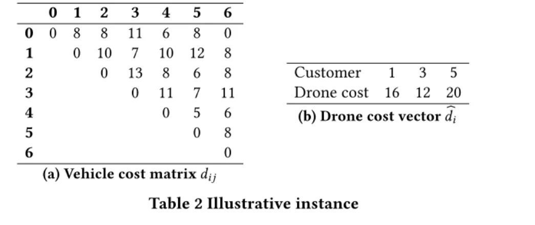
Figure 4 shows an illustrative example for an instance with 5 customers. Customers 2 and 4 are not drone-eligible. The vehicle travel cost matrix is reported in Table 2(a) in which we add the copy of the depot (node 6). Table 2(b) presents the drone-trip costs for drone-eligible customers. We assume τ = (1, 2, 3, 4, 5).

0 1 2 3 4 5 6 0 0 8 8 11 6 8 0 1 0 10 7 10 12 8 2 0 13 8 6 8 3 0 11 7 11 4 0 5 6 5 0 8 6 0

(a) Vehicle cost matrixdij

Customer 1 3 5

Drone cost 16 12 20

(b) Drone cost vector bdi

Table 2 Illustrative instance

The set of paths from 0 to n + 1 in Gτ _{exactly matches the set of acceptable routes for the vehicle that can be} extracted from sequence τ . Furthermore, given a path P, the cost vector (c1_{(P), c}2_{(P)) = (Í(i, j)∈Pc}1

ij, Í(i, j)∈Pc2ij) corresponds to the costs of the vehicle and the drone, if the route of the vehicle follows P and the remaining

0 8,0 1 10,0 2 13,0 3 11,0 4 5,0 5 8,0 6

8,16 8,12 6,20

Figure 4 GraphGτ for the instance of tables 2(a) and 2(b), withτ = (1, 2, 3, 4, 5).

customers are assigned to the drone. Taking again the example depicted with Figure 4, path P = (0, 2, 4, 5, 6) should be interpreted as a solution S with a vehicle tour (0, 2, 4, 5, 0) and customers 1 and 3 assigned to the drone; c1_{(P) = 29,} c2_{(P) = 28, c(S) = max(29, 28) = 29.}

For that reason, the aim of the split procedure is to find the path P from 0 to n + 1 in Gτ _{that minimizes} max(c1_{(P), c}2_{(P)). We now describe the dynamic programming procedure developed to compute this path.}

Dynamic programming scheme.To understand the procedure applied to find that shortest path, let us first consider the following definitions:

• partial path: a path going from 0 (origin depot) to any node i of graph Gτ_;

• label: the cost vector (c1_{, c}2_{)of a partial path calculated by adding the costs of the crossed arcs.}

The shortest path is found by applying the procedure described in Algorithm 2. The principle is to progressively associate a list of labels L(i) with each node i of Gτ_{. At the initialization, L(i) is set to ∅ for every node i (Line 1).} The procedure then starts by assigning label (0, 0) to L(0) (Line 2).

The procedure goes through the graph from the origin depot node 0 to the destination depot node n + 1 by following the order defined in sequence τ . Function increment on Line 5 is introduced for this purpose. For a given vertex i, list L(i) is constructed by adding a new label for every label in the list of labels of a predecessor node (Lines 6-13). The new label is simply defined by adding the arc cost (Line 8). In order to limit the number of labels generated in the lists as the procedure advance in the graph, some bounding mechanisms (Line 9) and a dominance rule (Line 10) are introduced. These two components are detailed below.

At the end, the shortest path is retrieved through a backtrack mechanism considering the best label found in L(n + 1). This shortest path constitutes the vehicle tour τ_vehicle and the nodes out of the path are assigned to the drone.

Dominance rule.The dominance rule is very simple. A label La = (ca1, c2a)dominates a label Lb = (c1_b, c_b2)if (c_a1 < c_b1 and c2

a ≤cb2) or (c1a ≤cb1 and ca2 < cb2). Before adding a new label to a list of label, dominance tests are tried with all the labels in the list, both to check whether the new label should be discarded or if an existing label should be removed.

The dominance rule guarantees that the number of labels attached to a node is limited by the number of values that can take label components c1_{or c}2_{. As this number can still be very large, bounding mechanisms are helpful to}

limit the combinatorial explosion.

Upper bound generation.The bounding mechanisms rely on the computation of several upper bounds. A first upper bound U B1is given by the value of the best solution found so far. A second upper bound U B2is obtained by applying Algorithm 2 with the following modifications:

• the bounding mechanisms of Line 9 are not considered;

• the dominance rule is changed to: La dominates Lb if c(La) ≤c(Lb); with this new rule, a single label is kept at each node of the graph.

Algorithm 2Procedure split(τ ) 1: L(i) ← ∅ for 0 ≤ i ≤ n + 1 2: L(0) ← {(0, 0)} 3: i ← 0 4: whilei <τ n + 1 do 5: increment i

6: for allj such that arc (j,i) ∈ Aτ do

7: for alllabel L ∈ L(j) do

8: L′_{← (c}1_{(L) + c}1

ji, c2(L) + c2ji)

9: ifL′is not pruned with the bounding mechanisms then

10: L(i) ← addW ithDominance(L(i), L′₎

11: end if

12: end for

13: end for

14: end while

15: bestLabel ← label L in L(n + 1) with minimum completion time max(c1(L), c2(L)) 16: τvehicle ←path that led to label bestLabel

17: τdrones ←nodes that are not in the path

0 8,0 1 10,0 2 13,0 3 11,0 4 5,0 5 8,0 6 8,16 8,12 6,20 (0,0) (8,0) (8,16) (21,16) (16,28) (21,28) (29,28) U B₂: (0,0) (8,0) (18,0) (18,12) (29,12) (34,12) (42,12) U B₃:

Figure 5 Upper bounds for the graph of Figure 4.

The third upper bound U B3results from the following greedy heuristic. The nodes are considered in the order

defined by <τ. Nodes are added to the vehicle tour τvehicle except when the two following conditions hold: node i

is drone-eligible and adding i to the drone does not increase the completion time of the current partial solution. In this case, node i is assigned to the drone. U B is set as the best (minimal) upper bound among these three bounds: U B = min(U B1,U B2,U B3).

Figure 5 represents the application of these algorithms to compute U B2and U B3on the example introduced with Figure 4. Assuming that no previous solution is known (U B1= +∞), we obtain U B2= 29, U B3= 42 and U B = 29. Lower bound generation.We introduce two lower bounds, LBtot(i) and LBveh(i), at each customer node of the graph. Lower bound LBtot_{(i) indicates the minimal total cost c}1_{(P) + c}2_{(P) of any path P between i and n + 1 in} Gτ_{. Lower bound LB}veh_{(i) indicates the minimal vehicle cost c}1_{(P) of any path P between i and n + 1 in G}τ_{. Both} bounds are computed simultaneously with a backward exploration of the acyclic (topologically-ordered) graph Gτ_.

Figure 6 details these lower bounds on the example introduced with Figure 4. Bounding mechanisms.We define the three following bounding rules:

• R1: prune label L if c2_{(L) ≥ U B}

0 8,0 1 10,0 2 13,0 3 11,0 4 5,0 5 8,0 6 8,16 8,12 6,20 0 0 8 8 6 13 17 24 14 33 24 43 22 51 LBveh_(i): LBtot_(i):

Figure 6 Lower bounds for the graph of Figure 4.

• R3: prune label L if c1_{(L) + c}2_{(L) + LB}tot_{(i) ≥ 2 × U B}

Rule R1 identifies labels whose completion time is already at least U B, because of the customers already assigned to the drone. Rule R2 identifies labels whose vehicle tour cannot finish before U B, because of the subtour already assigned to the vehicle and the minimal remaining path to n + 1. Rule R3 considers both the vehicle and drone completion times. It is based on the fact that whatever the path P extending the subpath associated with L to n + 1, the completion time of the resulting solution is max(c1_{(L) + c}1_{(P), c}2_{(L) + c}2_{(P)) ≥} c1(L)+c1(P )+c2(L)+c2(P )

2 ≥

c1(L)+c2(L)+LBt ot(i)

2 .

Hence, none of the labels for which R1, R2 or R3 holds, can result in a solution better than U B. They can be pruned.

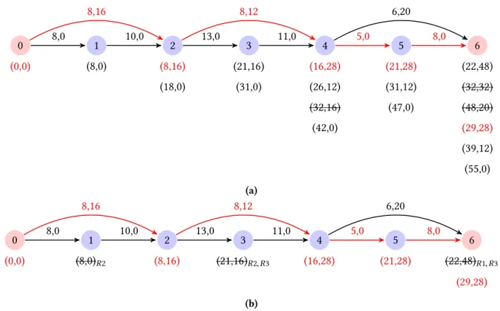
Figure 7 illustrates the split subroutine on the graph presented in Figure 4. List L(i) is reported under every node i. In Figure 7(a), the bounding mechanisms are not applied. Labels can only be removed by dominance. Dominated labels are crossed out. In Figure 7(b), the bounding mechanisms are reinserted. The bounding rule(s) enabling to delete a label is reported on the right of the strikethrough label.

In both cases, the optimal path and the associated labels are represented in red. The optimal decomposition is to assign customer sequence (2, 4, 5) to the vehicle and customers (1, 3) to the drone. The cost of this solution is 29.

4.3

Decoding procedure when

M > 1

When M > 1, the preceding decomposition scheme could naturally be adapted by defining labels of size M +1, where the first field represents the vehicle cost and the following M fields represent the cost for each drone. This would however induce a more complex labeling algorithm and, above all, many more labels, with probably intractable computing times except for fairly small instances. We preferred to handle this situation with a different approach.

We reproduce exactly Algorithm 2 with the sole modification that arc costs c2

ij are divided by M. This change simulates the fact that the total drone delivery time can be shared equally between the M drones. In other words, it also means that the PMS problem is relaxed, allowing both preemption of tasks and parallel execution of these tasks. Sequence τdrones returned by procedure split is then transformed into a feasible PMS solution (τ₁opt, . . . , τ_Mopt) with a greedy heuristic. We propose to apply the well known Longest Processing Time (LPT) heuristic [24]. In LPT, the tasks (drone deliveries) are first sorted in the decreasing order of their processing time (bdi). Then, they are successively assigned to the drone with the minimal current completion time.

5

EXPERIMENTS AND RESULTS

We conducted two sets of experiments. In the first set, we evaluate the efficiency of our heuristic on Murray and Chu [19]’s benchmark instances and present some further analyzes. As far as we know, these instances are the only

0 8,0 1 10,0 2 13,0 3 11,0 4 5,0 5 8,0 6 8,16 8,12 6,20 (0,0) (8,0) (8,16) (18,0) (21,16) (31,0) (16,28) (26,12) (32,16) (42,0) (21,28) (31,12) (47,0) (22,48) (32,32) (48,20) (29,28) (39,12) (55,0) (a) 0 8,0 1 10,0 2 13,0 3 11,0 4 5,0 5 8,0 6 8,16 8,12 6,20 (0,0) (8,0)R2 (8,16) (21,16)R2,R3 (16,28) (21,28) (22,48)R1,R3 (29,28) (b)

Figure 7 Illustration of thesplit procedure on the graph of Figure 4, without or with the bounding mech-anisms.

ones existing for this problem. Unfortunately, they are of small size (10 to 20 customers) and it is difficult to draw definitive conclusions with them. For this reason, we introduced instances of larger size on which we conducted a second set of experiments. In this second set, we investigate in more details the behavior of our heuristic and analyze the benefits of using drones.

The environment used for the computational work is Intel core(TM) i5-6200U CPU @ 2.30Ghz 2.40Ghz; 8GB RAM; Windows 10; 64 bits. C++ language is used for the implementation part.

For the experiments, we considered two different ways of applying our two-step heuristic: (1) Single-start two-stepH: the algorithm is executed exactly as it is described in Section 4.

(2) Multi-start two-stepH: the algorithm is repeated several times, with a randomized initialization and until a time limit is reached. Randomization is introduced in the nearest neighbor heuristic, by randomly selecting one of the K closest neighbors instead of the closest. The solution returned is the best solution among all the solutions found. In the experiments, we arbitrarily set K = 3. The computing time limit depends on the experiments and is indicated when needed.

5.1

First set of experiments: Murray and Chu’s instances

Murray and Chu [19]’s instances were generated with either 10 or 20 customers. The vehicle and drone speeds were fixed at the same speed of 25 miles/h. However, distances were computed with a Manhattan distance for the vehicle and with an Euclidean distance for the drones. The depot location was selected as being either near the center of all customers, near the edge of the customer region, or at the origin. Customer locations were generated

such that either 20%, 40%, 60% or 80% of all customers were located within the drone’s range from the depot, with the drone having a flight endurance of 30 min. Finally 10-20% of customers were arbitrarily set as not drone-eligible because of excessive parcel weights. Each of the above parameter settings was repeated 10 times, resulting in 120 instances with 10 customers and 120 instances with 20 customers. All these instances were solved with a single truck and either 1, 2 or 3 available UAVs, resulting in 720 test instances.For these instances, completion times are indicated in minutes.

Before analyzing the performance of our heuristic, let us recall the principle of Murray and Chu [19]’s PDSTSP heuristic. Their idea is to first assume that the drones will serve all the drone-eligible customers and that all remaining customers will be delivered by the vehicle. Based on this partition, a TSP and a PMS are solved for the vehicle and the drones, respectively. An improvement step reassigns individual customers to either a drone or the vehicle if it allows decreasing the overall completion time. This improvement step is implemented as follows. If the completion time for the drones exceeds the duration of the vehicle tour, a customer is moved from a drone to the vehicle. The move affording the greatest net savings is chosen. If no move yields a savings in the overall completion time a swap is investigated. The swap operator explores all pairwise exchanges of customers between the drones and the vehicle. If the completion time for the vehicle determines the overall completion time, the swap operator is again employed. The process of reallocating customers between the drones and the vehicle is repeated as long as improvements are carried out. Three TSP solution methods were evaluated for computing the vehicle tour, namely: integer programming (with the guarantee that the optimal TSP solution is obtained), the savings heuristic [18], and the nearest neighbor heuristic. Similarly, two PMS solution methods were evaluated for the drones: integer programming (exact solution) and the longest processing time (LPT) heuristic [24].In Murray and Chu’s experiments, mixed integer linear programs were solved with Gurobi version 5.6.0.

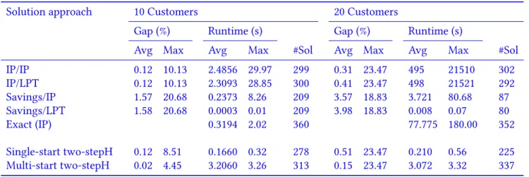
Table 3 presents a summary on the performance of our heuristics compared to Murray and Chu’s. The first four lines correspond to Murray and Chu’s methods. Note that we ignored the less efficient among their methods in this table. The fifth line provides information on the computation of exact solutions by Murray and Chu with their IP formulation. The results obtained with our two-step heuristic are presented for both single-start two-stepH and multi-start two-stepH, with a time limit of 3 seconds for the latter. Columns #Sol give the number of times each method found the best solution among all methods. Columns Gap give the average and maximal gaps to these best solutions, for each method. Columns Runtime report computing times, in seconds.

Table 3 Comparison with Murray and Chu results

Solution approach 10 Customers 20 Customers

Gap (%) Runtime (s) Gap (%) Runtime (s)

Avg Max Avg Max #Sol Avg Max Avg Max #Sol IP/IP 0.12 10.13 2.4856 29.97 299 0.31 23.47 495 21510 302 IP/LPT 0.12 10.13 2.3093 28.85 300 0.41 23.47 498 21521 292 Savings/IP 1.57 20.68 0.2373 8.26 209 3.57 18.83 3.721 80.68 87 Savings/LPT 1.58 20.68 0.0003 0.01 209 3.98 18.83 0.008 0.07 80 Exact (IP) 0.3194 2.02 360 77.775 180.00 352 Single-start two-stepH 0.12 8.51 0.1660 0.32 278 0.51 23.47 0.210 0.56 225 Multi-start two-stepH 0.02 4.45 3.2060 3.26 313 0.15 23.47 3.072 3.32 337

Regarding best solutions, Murray and Chu [19] indicate that their IP formulation was able to find the optimal solution for all of the 10-customer instances but was not able to solve in the imparted time 87 of the 360 20-customer

instances. Column #Sol however shows that for these 87 instances, IP still found the best solution among all tried methods in all cases except 8.

We observe that the single-start version of the two-step heuristic and the Savings/LPT are both extremely fast. In comparable amounts of time, single-start two-stepH is able to achieve far better optimality gaps than Savings/LPT. Regarding the multi-start version, we can notice that with a time limit of only 3 seconds, the two-step heuristic yields very small optimality gaps. The IP/IP and IP/LPT methods are also effective but very slow. In general, this comparison shows that our two-step descent algorithm is able to converge very quickly towards very good solutions, at least for small instances with 10 or 20 customers.

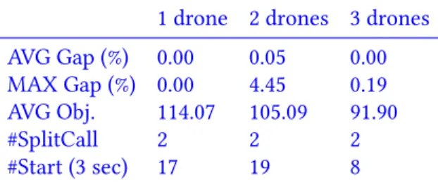
Table 4 and Table 5 show in more details the behavior of Multi-start two-stepH with 1, 2 or 3 drones for instances with 10 and 20 customers, respectively.

Table 4 Multi-start two-stepH (time limit: 3 sec) performance on 10 customer instances

1 drone 2 drones 3 drones AVG Gap (%) 0.00 0.05 0.00 MAX Gap (%) 0.00 4.45 0.19 AVG Obj. 114.07 105.09 91.90 #SplitCall 2 2 2 #Start (3 sec) 17 19 8

Table 5 Multi-start two-stepH (time limit: 3 sec) performance on 20 customer instances

1 drone 2 drones 3 drones AVG Gap (%) 0.20 0.06 0.18 MAX Gap (%) 23.47 2.41 6.33 AVG Obj. 141.90 139.93 139.82 #SplitCall 2 2 2 #Start (3 sec) 15 16 15

We notice that the average completion time value decreases when the number of drones increases. This is a logical expected result but it greatly depends on the number of drone-eligible customers and it is not always very significant. At some points, indeed, all the drone-eligible customers might be assigned to drones; then, if the vehicle tours is longer than drone tours, adding new drones does not help. Results also show that the split procedure is called 2 times on average.

Seeing that our decoding scheme is optimal when M = 1 (a single drone) while it is not when M > 1, we could have also expected larger gaps for instances with several drones. This is however not clearly observed with these results, probably showing the quality of the approximation introduced in the multiple-drones case.

5.2

Second set of experiments: new instances generated from TSPLIB

To evaluate our heuristic on larger instances, we generated another set of instances by using TSPLIB files att48.tsp, berlin52.tsp, eil101.tsp, gr120.tsp, pr152.tsp and gr229.tsp. The number in the file name corresponds to the number of customers which are represented by their coordinates x and y. To stay consistent with Murray and Chu’s instances, we used the Manhattan distance for the vehicle trip and the Euclidean distance for the drone trip. From each file, we

generated what we call a reference instance and several instances that can be derived from this reference instance by changing some parameters. These instances are characterized by:

• The position of the depot: A fictitious point was added to represent the depot. The depot location was selected as being either near the center of all customers (x0= maxi ∈N(xi)−₂mini ∈N(xi), y0= maxi ∈N(yi)−₂mini ∈N(yi)) or at the left-bottom corner of the region (x0= mini ∈N(xi), y₀= mini ∈N(yi)). In reference instances, the depot is located at the center.

• The percentage of drone-eligible customers: Instances were generated with either 0%, 20%, 40%, 60%, 80% or 100% of drone-eligible customers. We proceeded as follows. Let K be the target percentage of drone eligible customers. We introduced L (L = 30%) the percentage of non-drone-eligible customers that are not drone-eligible because of parcel weights. We selected these customers according to their index n: customers not drone-eligible because of their parcel weight are customers such that n (mod ⌊ 1

(1−K)×L⌋)= 0. Remaining customers were then set as drone-eligible in the increasing order of their distance to the depot, until reaching K% of drone-eligible customers. In reference instances, K = 80%.

• The drone speed: The drone can go at the same speed as the vehicle or 2, 3, 4 or 5 times faster. In this case, vector bd is simply divided by the speed factor. In the reference instances, the speed factor is 2.

• The number of drones: The drone fleet can be composed of 1, 2, 3, 4 or 5 drones. In the reference instance, a single drone is used.

Note that the method for generating drone-eligible customers might appear a little bit twisted, but it has the advantage of being fully deterministic and easily reproducible.

The first goal with these new instances is to conduct some sensitivity analyzes. We compare solutions obtained while changing the depot position, the percentage of drone-eligible customers, the drone speed factor and the number of drones, respectively. For that purpose, we consider the 6 reference instances and construct new instances by changing a single parameter at a time. The method used for these experiments is Multi-start two-stepH with a time limit set to 5 minutes (a large amount of time is given so as to obtain optimality gaps as small as possible and make the results more reliable).

Results are presented in tables 6 to 9. In these tables, columns labeled with C.T. indicate the value of the completion time and columns labeled with #D.C. indicate the number of customers assigned to the drones.

Table 6 investigates the impact of the depot location. We observe that completion times are higher when the depot is located at the left-bottom corner. Furthermore less customers are assigned to the drone. These observations are consistent with expectations.

Table 6 Impact of depot position (80% of drone-eligible customers, 1 drone, speed factor 2)

Instance Center Corner

C.T. #D.C. C.T. #D.C. att48 29954 17 33798 9 berlin52 6386.48 18 7830 8 eil101 564 28 650 19 gr120 1414 30 1730 18 pr152 76008 20 76556 19 gr229 1794.84 25 1913.74 9

In complement to this table, we also investigate if the drones tend to serve customers near the depot, in other words if there are any “rules of thumb” that dictate which customers should be served by the drones. Figure 8 shows

Figure 8 Results of the two-step heuristic for the 6 reference instances

the solutions obtained for our 6 reference instances (depot position: center, 80% of drone-eligible customers, drone speed: 2, one drone). The depot is represented by a triangle. Customers that are not drone-eligible are represented by squares and drone-eligible customers are represented by circles. The circle is in plain when the given drone-eligible customer is served by the drone. Images show no clear correlation between the position of a drone-eligible customer and its selection for a delivery by a drone.

Table 7 investigates the impact of the percentage of drone-eligible customers. The table shows that, in general, completion times are improved when the percentage of drone-eligible customers increases. However, it does not necessarily imply that the number of customers assigned to the drone increases (except of course for the case with 0 drone-eligible customers). Actually, at first, when a few customers are drone-eligible, they tend to be assigned to the drone to relieves the vehicle. Then, when a good balance in vehicle and drone completion times is reached, two conflicting phenomena are met: adding drone-eligible customers allows a better partition of the customers between the vehicle and the drone, and thus should result in an higher number of drones visited per unit of time; but, it also allows decreasing completion times, and thus should result in a smaller total number of customers assigned to the drone.

Table 7 Impact of the percentage of drone-eligible customers (depot at the center, 1 drone, speed factor 2) Instance 0% 20% 40% 60% 80% 100% C.T. #D.C. C.T. #D.C. C.T. #D.C. C.T. #D.C. C.T. #D.C. C.T. #D.C. att48 42136 0 38662 7 31592 15 30788.80 16 29954 17 27784 16 berlin52 9675 0 9350 4 8300 15 7410 25 6386.48 18 6180 14 eil101 819 0 738 18 646 31 578 27 564 28 561.41 26 gr120 2006 0 1736 18 1624 25 1494 29 1414 30 1414.80 23 pr152 86596 0 82504 22 77372 23 76786 20 76008 20 74468 23 gr229 2020.16 0 1862.76 19 1828.02 22 1807.50 23 1794.84 25 1498.05 11

In Table 8 and Table 9, we vary the speed and number of drones, respectively. We can notice that when the speed of the drone increases, the completion time is improved and the drone is able to visit more customers. Similar results are obtained when increasing the number of drones. Actually, this is not a surprise seeing that in the algorithm, changing the speed or the number of drones almost has the same effect. For example, the only difference between solving an instance with 2 drones having a speed ratio 2 and an instance with 1 drone of speed ratio 4, concerns the solution of the PMS. However, one should mention that when the number of drones increases the average number of customers assigned to each drone decreases. Finally, in some cases, adding drones does not allow improving the solution, for the reasons already developed in Section 5.1 (see att48 and berlin52).

Table 8 Impact of the drone speed (depot at the center, 80% of drone-eligible customers, 1 drone)

Instance 1 2 3 4 5 C.T. #D.C. C.T. #D.C. C.T. #D.C. C.T. #D.C. C.T. #D.C. att48 33234 10 29954 17 29142 21 28686 24 28610 26 berlin52 7450 13 6386.48 18 5656.56 23 5290.65 31 5190 35 eil101 650 17 564 28 504 36 456 39 420.83 47 gr120 1592 18 1414 30 1289.27 37 1189.71 43 1112 50 pr152 80164 12 76008 20 72936 31 70412 41 67798 31 gr229 1865 13 1794.84 25 1735.16 36 1679.33 48 1642.04 58

Table 9 Impact of the number of drones (depot at the center, 80% of drone-eligible customers, speed factor 2) Instance 1 2 3 4 5 C.T. #D.C. C.T. #D.C. C.T. #D.C. C.T. #D.C. C.T. #D.C. att48 29954 17 28686 24 28610 26 28610 26 28610 27 berlin52 6386.48 18 5299.81 31 5290 35 5190 35 5190 35 eil101 564 28 456 40 395 52 346.68 59 319.74 69 gr120 1414 30 1188.51 43 1044.65 54 946.04 65 880 73 pr152 76008 20 70244 42 65062.10 41 60027.40 56 56336.10 60 gr229 1794.84 25 1686.75 50 1603.90 66 1518.62 84 1483.68 98

With further experiments, we analyze the behavior of our two-step heuristic general scheme. For these experiments, we only consider the reference instance obtained from gr229.tsp and execute Single-start two-stepH. Results are presented in Tables 10 and 11.

Table 10 presents the results obtained while varying the percentage of drone-eligible customers. It provides the value of the completion time, the average number of calls to the split procedure, the average number of labels generated in the split procedure (summed over all nodes and including labels eventually deleted by dominance or with the bounding mechanisms) and the percentage of labels deleted with the bounding mechanisms.

Table 10 Impact of the percentage of drone-eligible customers on the behavior of Single-start two-sepH (depot at the center, 1 drone, speed factor 2)

Drone-eligible C.T. #SplitCall #LabelsGenerated. LabelsDeleted (%) 0% 2020.16 0 0 0 20% 1867.60 3 9450 28.26 40% 1826.22 6 32969 53.10 60% 1812.84 6 139849 76.85 80% 1809.84 4 385309 88.43 100% 1500.45 4 3662748 99.05

Several interesting conclusions can be drawn from this table. First, one can observe an increase in the number of calls to the split procedure following that of the number of drone-eligible customers. It indicates that, thanks to the flexibility provided by the new drone-eligible customers, the method gets less easily trapped into a local optimum. However, the method still converges quickly (a few iterations) and towards good-quality solutions: the gaps with the solutions found in 5 minutes with Multi-start two-stepH (last line of Table 7) remain limited. Second, one can see a quick increase in the number of generated labels. It can clearly be explained by the shape of graph Gτ_{. Having} more drone-eligible customers favors longer arcs and result in more arcs in the graph, and thus more possibilities for extending labels. Fortunately, bounding mechanisms are capable of getting rid of most of these labels: more than 99% when all the customers are drone-eligible.

Table 11 investigates the quality of the approximation made in the split procedure when M > 1. It shows the average and maximum gaps between the drone completion time found by the split procedure (assuming a single drone with a speed multiplied by M) and the completion time obtained after having applied the LPT heuristic. We observe that the gaps grow when the number of drones increases, but remain very limited.

Table 11 Average gap between the drone completion time found by the split procedure and the comple-tion time found with the LPT heuristic

Number of drones 1 2 3 4 5 Avg Gap (%) 0 0.01 0.73 0.85 0.99 Max Gap (%) 0 0.01 1.41 1.35 1.86

Finally, with Table 12, we provide a benchmark set of best known solutions on our new instances, for future researches. In this table, we consider our 6 references instances with a drone fleet size going from 1 to 5 drones. It gives rise to a new instance set of 30 instances. The results provided in the table were obtained with a single execution of Multi-start two-stepH with a time limit of 5 minutes.

Table 12 Benchmark based on reference instances with 1 to 5 drones applying Multi-start two-setpH with a time limit of 5 mins

1 2 3 4 5 att48 29954 28686 28610 28610 28610 berlin52 6386.48 5299.81 5190 5190 5190 eil101 564 456 395 346.68 319.74 gr120 1414 1188.51 1044.65 946.04 880 pr152 76008 70244 65062.10 60027.40 56336.10 gr229 1794.84 1686.75 1603.90 1518.62 1483.68

6

CONCLUSIONS

Drone deliveries look like the future: unmanned aerial vehicles rapidly delivering packages to our doors, eliminating both waiting times and the cost of human labor.

In this paper, we studied the combination of vehicle and drones for parcel delivery in a approach without synchronization between the vehicle and drones. We proposed an iterative two-steps heuristic that uses dynamic programming for efficiently partitioning the customers between the vehicle and the drone fleet. Results are very promising and permit a clear improvement over the existing literature.

Nevertheless, there are still a lot of possible improvements. First, we mainly focused in this study on the split procedure. Clearly the quality of the results could be slightly improved by solving better the PMS that are repeatedly solved in the solution scheme. In the current implementation, the algorithms used for solving these problems are very simple. They have the advantage to be very quick, but it is certainly possible to gain in effectiveness with a limited increase in computing times. Most importantly, the iterative algorithm could certainly beneficially be inserted within a metaheuristic scheme. Multi-start two-stepH can already be interpreted as a GRASP, but more promising metaheuristic schemes exist. Iterated Local search, or the hybridization with evolutionary algorithms, would for example be natural candidates.

Apart from these issues, another clear limit in the evaluation of our method is the lack of lower bounds (except for small instances for which the optimal solution is known). Developing an efficient solution method, as branch-and-cut or branch-and-price, or finding tight lower bounds is certainly an important direction to follow. Branch-and-cut solution procedures have been developed for other types of routing problems where a single truck selects and visits a subset of customers (e.g., the Selective TSP [11] or the Profitable Tour Problem [15]). The valid inequalities and separation algorithms used in these procedures could certainly be generalized to our problem.

Finally, more complex variants of the problem would certainly deserve to be addressed. Especially, a strong limit in the problem definition is the presence of a single vehicle. Parcel delivery typically involves many vehicles. Extending the problem to this setting would certainly be valuable, though raising new difficulties in the partitioning subproblem.

ACKNOWLEDGMENTS

The authors would like to thank Chase Murray and Amanda Chu for providing their instances and their results.

REFERENCES

[2] DHL International GmbH. (2014, Sep.) DHL parcelcopter launches initial operations for research purposes. [Online]. Avail-able :http://www.dhl.com/en/press/releases/releases_2014/group/dhl_parcelcopter_launches_initial_operations_for_research_purposes. html. (2014).

[3] Australia Post tests drones for parcel delivery. [Online]. Available : http://www.smh.com.au/technology/innovation/ australia-post-tests-drones-for-parcel-delivery-20160415-go77a4.html. (2016). 15 April 2016.

[4] The Future of Healthcare is Out for Delivery. [Online]. Available :http://flyzipline.com/product/. (2016).

[5] L’avenir est dans le ciel : Domino’s et Flirtey s’associent pour livrer des pizzas par drone, conformÃľment au code de l’aviation. [Online]. Available :https://pizza.dominos.fr/dominos-pizza/dru-drone-dominos-et-flirtey-livraison-de-pizzas. (2016). 25 August 2016. [6] Niels Agatz, Paul Bouman, and Marie Schmidt. 2015. Optimization approaches for the traveling salesman problem with drone. ERIM

Report Series Reference No. ERS-2015-011-LIS(2015).

[7] João Carlos Namorado Climaco and Ernesto Queirós Vieira Martins. 1982. A bicriterion shortest path algorithm. European Journal of Operational Research11, 4 (1982), 399–404.

[8] Kevin Dorling, Jordan Heinrichs, Geoffrey G Messier, and Sebastian Magierowski. 2016. Vehicle routing problems for drone delivery. IEEE Transactions on Systems, Man, and Cybernetics: Systems(2016).

[9] Claudio Gambella, Andrea Lodi, and Daniele Vigo. 2017. Exact Solutions for the Carrier–Vehicle Traveling Salesman Problem. Transportation Science(2017).

[10] Emanuele Garone, Roberto Naldi, and Alessandro Casavola. 2011. Traveling-Salesman Problem for a Class of Carrier-Vehicle Systems. Journal of Guidance Control and Dynamics34, 4 (2011), 1272.

[11] Michel Gendreau, Gilbert Laporte, and Frederic Semet. 1998. A branch-and-cut algorithm for the undirected selective traveling salesman problem. Networks 32, 4 (1998), 263–273.

[12] Quang Minh Ha, Yves Deville, Quang Dung Pham, and Minh Hoàng Hà. 2015. Heuristic methods for the Traveling Salesman Problem with Drone. arXiv preprint arXiv:1509.08764 (2015).

[13] Quang Minh Ha, Yves Deville, Quang Dung Pham, and Minh Hoàng Hà. 2015. On the Min-cost Traveling Salesman Problem with Drone. arXiv preprint arXiv:1512.01503 (2015).

[14] Keld Helsgaun. 2000. An effective implementation of the Lin–Kernighan traveling salesman heuristic. European Journal of Operational Research126, 1 (2000), 106–130.

[15] Mads Kehlet Jepsen, Bjørn Petersen, Simon Spoorendonk, and David Pisinger. 2014. A branch-and-cut algorithm for the capacitated profitable tour problem. Discrete Optimization 14 (2014), 78–96.

[16] Leo Kelion. Alibaba begins drone delivery trials in China. [Online]. Available :http://www.bbc.com/news/technology-31129804. (2015). 4 February 2015.

[17] Andrew Liptak. 7-Eleven just made the first commercial delivery by drone. [Online]. Available ::http://www.theverge.com/2016/7/23/ 12262468/7-11-first-retailer-deliver-food-drone. (2016). 23 July 2016.

[18] Jens Lysgaard. 1997. Clarke & Wright’s Savings Algorithm. (1997).

[19] Chase C Murray and Amanda G Chu. 2015. The flying sidekick traveling salesman problem: Optimization of drone-assisted parcel delivery. Transportation Research Part C: Emerging Technologies 54 (2015), 86–109.

[20] Rodrique Ngowi. = UPS testing drones for use in its package delivery system. [Online]. Available :http://phys.org/news/ 2016-09-ups-drones-package-delivery.html. (2016). 23 September 2016.

[21] Andrea Ponza. 2016. Optimization of Drone-assisted parcel delivery. (2016).

[22] Marlin W Ulmer and Barrett W Thomas. Same-Day Delivery with a Heterogeneous Fleet of Drones and Vehicles. (2017). preprint on webpage at https://www.researchgate.net/publication/301739923_The_vehicle_routing_problem_with_drones_Several_worst-case_ results.

[23] Xingyin Wang, Stefan Poikonen, and Bruce Golden. 2016. The vehicle routing problem with drones: several worst-case results. Optimization Letters(2016), 1–19.